Accurate Measurement Method for Distribution Parameters of Four-Circuit Transmission Lines with the Same Voltage Considering Earth Resistance

Abstract

In response to the limitations of existing parameter measurement methods for four-circuit transmission lines of the same voltage—namely, the failure to account for earth resistance and the complexity of methods that hinder live-line measurements—this paper proposes a more accurate method for measuring the distribution parameters of such transmission lines, incorporating earth resistance. The paper derives the transmission equations, including earth resistance, from the standard transmission line equations for three-phase power lines. The symmetrical component method is employed to decouple the parameters, allowing the earth resistance, which is difficult to measure directly, to be expressed as a combination of positive and zero-sequence parameters that are easier to measure. Additionally, the phase-mode transformation matrix for the four-circuit line parameters is derived, enabling the diagonalization of the twelve-order parameter matrix for the four-circuit lines. This transformation matrix can then be applied to the voltage and current signals measured at both ends of the line, facilitating the determination of the voltage and current magnitudes. At each magnitude, the relationship between voltage and current conforms to the transmission equations of a single-circuit line. The proposed method is compared with traditional methods and improved traditional methods using PSCAD/EMTDC software (version 4.6.2). Furthermore, an adaptability analysis of the proposed method is conducted, considering variations in line length and theoretical initial values. The results demonstrate that the proposed method is suitable for measuring the distribution parameters of four-circuit transmission lines of the same voltage across a range of voltage levels and line lengths.

1. Introduction

In response to the dual carbon goals of “carbon neutrality and peak carbon emissions”, the construction of a new power system has become an urgent priority [1,2]. This system requires substantial changes across all stages, including generation, transformation, transmission, distribution, and consumption [3,4]. However, the long-standing neglect of grid infrastructure development has resulted in a significant deficit in the capacity for large-scale inter-regional power transmission. The existing transmission systems are unable to efficiently deliver renewable energy to load aggregation areas, leading to substantial resource wastage [5,6]. Accurate determination of the power-frequency parameters of transmission lines is crucial for the stable and safe operation of the power system [7,8,9,10,11]. To meet the growing electricity demand in China, the expansion of transmission lines has been ongoing. Due to limited land resources, multi-circuit parallel transmission lines have become the preferred solution [12,13,14]. While multi-circuit parallel lines enhance transmission capacity, they also intensify the electromagnetic coupling between lines. Combined with the influence of various environmental factors, the theoretical values of transmission line parameters derived from the Carson formula often deviate significantly from actual line parameters [15]. In this context, direct measurement of line parameters has emerged as the only reliable method for obtaining accurate parameters [16].

The parameters of the transmission line’s earth return loop directly reflect the state of the earth loop. However, research on the measurement of earth loop parameters has been largely overlooked by academia. Due to the presence of soil resistivity, the earth loop cannot be modeled as an ideal conductor. In certain extreme environments, the earth loop significantly influences the voltage and current distribution of overhead lines. Furthermore, when soil resistivity is high, current losses in the earth loop cannot be neglected. Therefore, precise measurement of earth resistance is vital for the normal operation of power systems [17].

Existing research on ground loop parameter measurement has explored various approaches, yet several limitations remain. In [18], a measurement model based on a single-circuit non-transposed transmission line was proposed, incorporating ground loop parameters. However, the model did not account for the mutual inductance between overhead conductors, and the self-impedance parameters of the three-phase system did not fully satisfy the asymmetry condition. In [19], a measurement model for double-circuit asymmetric transmission lines was developed, considering the influence of the ground loop on collected signals. Nevertheless, the study did not include direct calculations of ground loop parameters.

Further advancements have been made in [20], where an improved single-conductor ground-return distributed parameter model was proposed, deriving an accurate expression for ground resistance, which was later validated through field experiments. Building upon this, studies in [21,22] extended the accurate measurement of ground resistance to multi-circuit AC transmission lines. However, these studies assumed that the ground resistance of each circuit was identical and focused solely on self-resistance measurements, which may not fully reflect practical operating conditions.

In the context of multi-circuit parallel transmission lines, the existing literature typically integrates the overhead conductor section and the ground return loop into a unified model, without isolating the measurement of ground loop parameters. Additionally, many studies adopt overly simplified assumptions regarding ground loop characteristics, failing to comprehensively analyze different types of ground resistance and their influencing factors. As a result, existing methods lack targeted measurement strategies for ground loops, highlighting the need for a more precise and systematic approach to measuring ground loop parameters in multi-circuit parallel transmission systems.

The main contributions of this paper are summarized as follows:

• A novel measurement method is proposed for the distribution parameters of four-circuit transmission lines with the same voltage, explicitly considering the impact of earth resistance, which has been largely neglected in previous studies.
• A phase-mode transformation matrix for four-circuit lines is derived, effectively decoupling the twelve-order parameter matrix and enabling a more efficient computation of voltage and current relationships.
• The proposed method is validated through numerical simulations in PSCAD/EMTDC, demonstrating its accuracy and applicability for various line lengths and voltage levels.
• A comparative analysis is conducted between the proposed method, traditional methods, and improved traditional methods, illustrating the superiority of the proposed approach in terms of measurement accuracy and computational efficiency.

The remainder of this paper is organized as follows: Section 2 presents the theoretical model of the four-circuit transmission line, considering the effects of earth resistance, and elaborates on the proposed measurement method, including the derivation of key equations. Section 3 describes the simulation setup and results, with a comparative analysis of different methods. Section 4 summarizes the key findings and outlines potential future research directions.

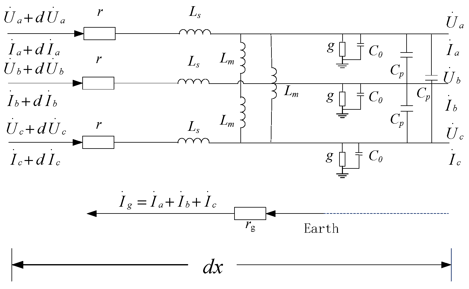
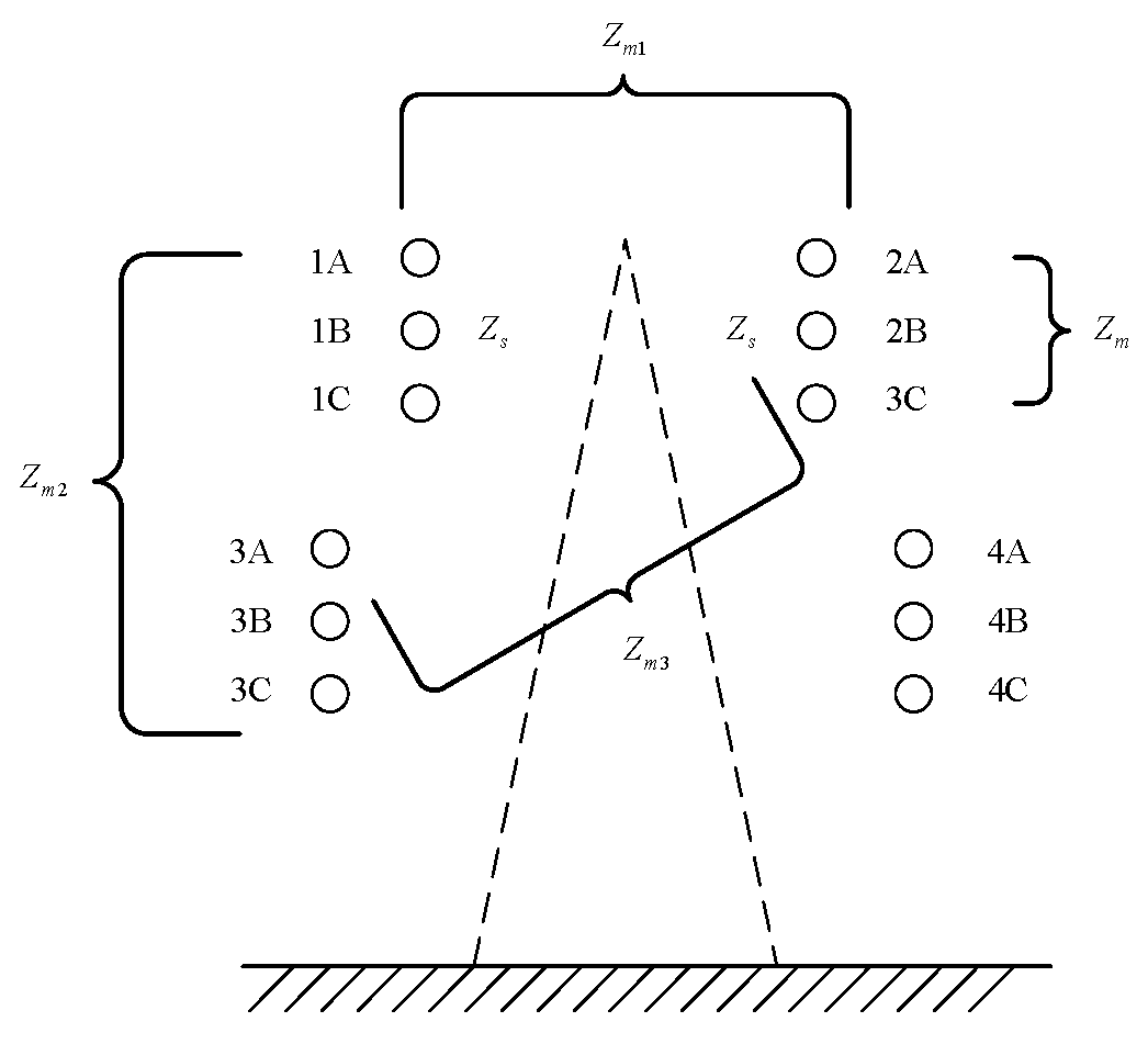
2. Three-Phase Parallel Line Model Considering Earth Return

The earth resistance of overhead lines serves as an indicator of the operational status of the line-earth return loop, directly affecting the voltage distribution and losses during power transmission. The distribution parameter model of a three-phase transmission line, accounting for earth resistance, is presented in Figure 1. It is assumed that the overhead line undergoes a full three-phase cycle switching, with the electrical relationships within the transmission line segment depicted in the diagram.

In Figure 1, $r$ represents the AC resistance of the overhead line, $L_s$ and $L_m$ denote the self-inductance and mutual inductance of the three-phase line, respectively, $g$ is the ground conductance of the overhead line, and $C_0$ and $C_p$ represent the self-capacitance and mutual capacitance of the three-phase line to the ground, respectively. $r_g$ represents the earth resistance corresponding to the ground return loop of this segment of the line.

According to Kirchhoff’s law, the voltage and current of this segment of the line element are related as follows:

$$\left\{\begin{array}{l}d{\dot{U}}_{abc}=Z_{abc}{\dot{I}}_{abc}dx\\ d{\dot{I}}_{abc}=Y_{abc}{\dot{U}}_{abc}dx\end{array}\right.$$

(1)

where ${\dot{U}}_{abc}={\left[\begin{array}{ccc}{\dot{U}}_a& {\dot{U}}_b& {\dot{U}}_c\end{array}\right]}^T$ and ${\dot{I}}_{abc}={\left[\begin{array}{ccc}{\dot{I}}_a& {\dot{I}}_b& {\dot{I}}_c\end{array}\right]}^T$ are the phase voltages and currents, respectively. $Z_{abc}$ and $Y_{abc}$ are the impedance and admittance matrices for the three-phase line, with the specific expressions as follows:

$$Z_{abc}=\left[\begin{array}{ccc}{r}_g+r+j\omega L_s& r_g+j\omega L_m& r_g+j\omega L_m\\ r_g+j\omega L_m& r_g+r+j\omega L_s& r_g+j\omega L_m\\ r_g+j\omega L_m& r_g+j\omega L_m& r_g+r+j\omega L_s\end{array}\right]$$

(2)

$$Y_{abc}=\left[\begin{array}{ccc}g+j\omega \left(C_0+2C_p\right)& -j\omega C_p& -j\omega C_p\\ -j\omega C_p& g+j\omega \left(C_0+2C_p\right)& -j\omega C_p\\ -j\omega C_p& -j\omega C_p& g+j\omega \left(C_0+2C_p\right)\end{array}\right]$$

(3)

For a three-phase line, the symmetrical component method is commonly used for analysis. In the case of a balanced three-phase line, the mutual coupling between phases a, b, and c can be transformed into three independent sequence components: positive sequence, negative sequence, and zero sequence. This transformation enables analysis within a single sequence component, thereby simplifying the overall analysis. The transformation matrix for the three-phase symmetrical component method is given by:

$$S=\left[\begin{array}{ccc}1& a^2& a\\ 1& a& a^2\\ 1& 1& 1\end{array}\right]$$

(4)

where $a=e^{j{120}^{°}}$.

For the three-phase line shown in Figure 1, applying the symmetrical component method for decoupling, the phase impedance and admittance matrices are transformed into the sequence impedance and admittance matrices, as follows:

$$\begin{array}{ll}{Z}_{120}& =S^{-1}{Z}_{abc}S\\ & =\left[\begin{array}{ccc}r+j\omega \left(L_s-L_m\right)& & \\ & r+j\omega \left(L_s-L_m\right)& \\ & & 3r_g+r+j\omega \left(L_s+2L_m\right)\end{array}\right]\end{array}$$

(5)

$$\begin{array}{ll}{Y}_{120}& =S^{-1}{Y}_{abc}S\\ & =\left[\begin{array}{ccc}g+j\omega \left(C_0+3C_p\right)& & \\ & g+j\omega \left(C_0+3C_p\right)& \\ & & g+j\omega 3C_0\end{array}\right]\end{array}$$

(6)

For Equation (5), the resulting positive-sequence self-impedance is:

$$Z_1=r+j\omega \left(L_s-L_m\right)$$

The zero-sequence self-impedance is:

$$Z_0=3r_g+r+j\omega \left(L_s+2L_m\right)$$

Thus, the earth resistance of the three-phase line can be calculated using Equation (7):

$$r_g={\displaystyle \frac{1}{3}}\times real\left(Z_0-Z_1\right)$$

(7)

Therefore, for a single-circuit line, as long as the positive-sequence and zero-sequence impedances of the line can be obtained, the earth resistance of the single-circuit line can be calculated using Equation (7).

2.1. Physical Model of Transmission Lines

In practical engineering applications, multi-circuit parallel transmission lines are widely used due to their high capacity and low loss characteristics. Among these, four-circuit lines on a common tower are preferred for their superior transmission capabilities. The tower structures for four-circuit lines on a common tower typically include configurations with three, five, or six crossarms.

For the transmission line shown in Figure 2.

Figure 2 illustrates the physical model of a four-circuit transmission line with the same voltage level. In this model, (1A, 1B, 1C), (2A, 2B, 2C), (3A, 3B, 3C), and (4A, 4B, 4C) represent the phase conductors of the four circuits, where “A”, “B”, and “C” correspond to the three-phase system of each circuit. These conductors are arranged symmetrically on a common transmission tower. The parameters $Z_m$, $Z_{m1}$, $Z_{m2}$, and $Z_{m3}$ represent the mutual impedance components between circuits at different distances: $Z_m$ denotes the mutual impedance between adjacent circuits. $Z_{m1}$, $Z_{m2}$, and $Z_{m3}$ represent the mutual impedance between non-adjacent circuits, increasing in distance from $Z_{m1}$ to $Z_{m3}$. The coupling of (4A, 4B, 4C) is not ignored but is inherently accounted for in the impedance matrix. Due to the symmetrical structure of the transmission tower, the mutual impedance relationships among all circuits can be fully described using $Z_m$, $Z_{m1}$, $Z_{m2}$, and $Z_{m3}$, ensuring a complete representation of electromagnetic interactions.

Additionally, the model assumes that the height of the conductors above the ground is significantly greater than the conductor dimensions. This allows the equivalent ground depth for all circuits to be considered approximately the same, and the vertical symmetry of the tower structure is maintained. For the physical model of the four-circuit line, the self-parameters of the line satisfy the following relationship:

$$\left\{\begin{array}{l}{Z}_a=Z_b=Z_c=Z_d=Z_s=R_s+j\omega L_s\\ Y_a=Y_b=Y_c=Y_d=Y_s=j\omega C_s\end{array}\right.$$

(8)

where $R_s$, $L_s$, and $C_s$ represent the self-resistance, self-inductance, and self-capacitance of each phase conductor, respectively. Since the admittance parameters are relatively small, they are neglected in this analysis. At the same time, the impedance parameters $Z_m$ and the admittance parameters $Y_m$ between each pair of circuits are also equal.

It is assumed that the three-phase lines are fully transposed, allowing the three-phase transmission lines to be treated as single-phase lines during analysis. As a result, the mutual parameters between any two circuits are identical to the phase parameters between corresponding phases in the two circuits. Furthermore, due to the symmetry of the tower structure, the mutual parameters between the lines satisfy the following relationship:

$$\left\{\begin{array}{l}{Z}_{ab}=Z_{cd}=Z_{m1}=R_{m1}+j\omega L_{m1}\\ Z_{ac}=Z_{bd}=Z_{m2}=R_{m2}+j\omega L_{m2}\\ Z_{ad}=Z_{bc}=Z_{m3}=R_{m3}+j\omega L_{m3}\\ Y_{ab}=Y_{cd}=Y_{m1}=j\omega C_{m1}\\ Y_{ac}=Y_{bd}=Y_{m2}=j\omega C_{m2}\\ Y_{ad}=Y_{bc}=Y_{m3}=j\omega C_{m3}\end{array}\right.$$

(9)

where $R_{mi}\left(i=1,2,3\right)$ is the mutual resistance between the lines, $L_{mi}\left(i=1,2,3\right)$ is the mutual inductance, and $C_{mi}\left(i=1,2,3\right)$ is the mutual capacitance.

The transmission line equations can be written as follows:

$$\left\{\begin{array}{l}{\displaystyle \frac{d\dot{U}}{dx}}=Z\dot{I}\\ {\displaystyle \frac{d\dot{I}}{dx}}=Y\dot{U}\end{array}\right.$$

(10)

where $\dot{U}={\left[\begin{array}{cccccc}{\dot{U}}_{1A}& {\dot{U}}_{1B}& {\dot{U}}_{1C}& \cdots & {\dot{U}}_{4B}& {\dot{U}}_{4C}\end{array}\right]}^T$ and $\dot{I}={\left[\begin{array}{cccccc}{\dot{I}}_{1A}& {\dot{I}}_{1B}& {\dot{I}}_{1C}& \cdots & {\dot{I}}_{4B}& {\dot{I}}_{4C}\end{array}\right]}^T$ represent the phase voltage and phase current applied to each of the four-circuit lines, respectively.

Both the series impedance matrix and the parallel admittance matrix are 12 × 12 square matrices, and their specific expressions are as follows:

$$Z={\left[\begin{array}{cc}{Z}_S& Z_M\\ Z_M& Z_S\end{array}\right]}_{12\times 12}$$

(11)

$$Y={\left[\begin{array}{cc}{Y}_S& Y_M\\ Y_M& Y_S\end{array}\right]}_{12\times 12}$$

(12)

As observed, in a four-circuit line on the same tower, the voltage or current on any given phase is influenced by the voltage and current on all other eleven phases, indicating a strong coupling between phases. Directly solving Equations (11) and (12) to obtain the line parameters would be computationally intensive. To address this issue, this paper proposes a decoupling method based on phase transformation, which effectively decouples the original parameter matrices and simplifies the calculation process.

Next, using the impedance parameter matrix from Equation (11) as an example, the derivation of the phase transformation matrix $T$ is introduced.

The impedance parameter matrix described using block matrices is expressed as $Z$, which is a typical two-phase system. The decoupling matrix for a two-phase system can be directly applied to transform it. The transformation expression is:

$$T_1^{-1}ZT=\left[\begin{array}{cc}{Z}_S+Z_M& \\ & Z_S-Z_M\end{array}\right]=\left[\begin{array}{cc}{Z}_1& \\ & Z_2\end{array}\right]$$

(13)

where $T_1=\left[\begin{array}{cc}I& I\\ I& -I\end{array}\right]$, $I$ represents the 6 × 6 identity matrix.

The expressions for $Z_1$ and $Z_2$ are as follows:

$$\begin{array}{cc}{Z}_1& =Z_S+Z_M\hfill \\ & =\left[\begin{array}{cccccc}{Z}_s+Z_{m2}& Z_m+Z_{m2}& Z_m+Z_{m2}& Z_{m1}+Z_{m3}& Z_{m1}+Z_{m3}& Z_{m1}+Z_{m3}\\ Z_m+Z_{m2}& Z_s+Z_{m2}& Z_m+Z_{m2}& Z_{m1}+Z_{m3}& Z_{m1}+Z_{m3}& Z_{m1}+Z_{m3}\\ Z_m+Z_{m2}& Z_m+Z_{m2}& Z_s+Z_{m2}& Z_{m1}+Z_{m3}& Z_{m1}+Z_{m3}& Z_{m1}+Z_{m3}\\ Z_{m1}+Z_{m3}& Z_{m1}+Z_{m3}& Z_{m1}+Z_{m3}& Z_s+Z_{m2}& Z_m+Z_{m2}& Z_m+Z_{m2}\\ Z_{m1}+Z_{m3}& Z_{m1}+Z_{m3}& Z_{m1}+Z_{m3}& Z_m+Z_{m2}& Z_s+Z_{m2}& Z_m+Z_{m2}\\ Z_{m1}+Z_{m3}& Z_{m1}+Z_{m3}& Z_{m1}+Z_{m3}& Z_m+Z_{m2}& Z_m+Z_{m2}& Z_s+Z_{m2}\end{array}\right]\end{array}$$

(14)

$$\begin{array}{cc}{Z}_2& =Z_S-Z_M\hfill \\ & =\left[\begin{array}{cccccc}{Z}_s-Z_{m2}& Z_m-Z_{m2}& Z_m-Z_{m2}& Z_{m1}-Z_{m3}& Z_{m1}-Z_{m3}& Z_{m1}-Z_{m3}\\ Z_m-Z_{m2}& Z_s-Z_{m2}& Z_m-Z_{m2}& Z_{m1}-Z_{m3}& Z_{m1}-Z_{m3}& Z_{m1}-Z_{m3}\\ Z_m-Z_{m2}& Z_m-Z_{m2}& Z_s-Z_{m2}& Z_{m1}-Z_{m3}& Z_{m1}-Z_{m3}& Z_{m1}-Z_{m3}\\ Z_{m1}-Z_{m3}& Z_{m1}-Z_{m3}& Z_{m1}-Z_{m3}& Z_s-Z_{m2}& Z_m-Z_{m2}& Z_m-Z_{m2}\\ Z_{m1}-Z_{m3}& Z_{m1}-Z_{m3}& Z_{m1}-Z_{m3}& Z_m-Z_{m2}& Z_s-Z_{m2}& Z_m-Z_{m2}\\ Z_{m1}-Z_{m3}& Z_{m1}-Z_{m3}& Z_{m1}-Z_{m3}& Z_m-Z_{m2}& Z_m-Z_{m2}& Z_s-Z_{m2}\end{array}\right]\end{array}$$

(15)

Upon inspecting Equations (14) and (15), the matrices $Z_1$ and $Z_2$, after the preliminary transformation, already have the same form as the parameter matrix $Z_S$ of a two-circuit line on the same tower. Based on the phase transformation matrix $T_2$ for a two-circuit line on the same tower [23], $Z_1$ and $Z_2$ can be decoupled into diagonal matrices, with the expression for $T_2$ as:

$$T_2=\left[\begin{array}{ccc}{\xi }_0& {\xi }_1& {\xi }_2\end{array}\right]$$

(16)

where ${\xi }_0=k_1{\left[\begin{array}{cccccc}1& 1& 1& 1& 1& 1\end{array}\right]}^T$, ${\xi }_1=k_2{\left[\begin{array}{cccccc}1& 1& 1& -1& -1& -1\end{array}\right]}^T$, $k_1$ and $k_2$ are constants, and ${\xi }_2$ is a 6 × 4 matrix, where the sum of the elements in each column is zero and the columns are linearly independent.

It can be proven that the columns of the transformation matrix $T_2$ are the eigenvectors of matrix $Z_1\left(Z_2\right)$, with the corresponding eigenvalues of ${\xi }_0$ and ${\xi }_1$ being simple roots, and the eigenvalue of ${\xi }_2$ being a quadruple root.

Therefore, the transformation matrix $T$ can be expressed as:

$$T=T_1\left[\begin{array}{cc}{T}_2& \\ & T_2\end{array}\right]=\left[\begin{array}{cc}I& I\\ I& -I\end{array}\right]\left[\begin{array}{cc}{T}_2& \\ & T_2\end{array}\right]=\left[\begin{array}{cc}{T}_2& T_2\\ T_2& -T_2\end{array}\right]$$

(17)

For convenience in computation, the columns of matrix $T$ are simplified using elementary column transformations. The expression for the transformation matrix $T$ becomes:

$$T=\left[\begin{array}{cccccccccccc}1& 1& 1& 1& 1& 1& 1& 1& 1& 1& 1& 1\\ 1& 1& 1& 1& 1& 1& -1& -1& -1& -1& -1& -1\\ 1& 1& 1& -1& -1& -1& 1& 1& 1& -1& -1& -1\\ 1& 1& 1& -1& -1& -1& -1& -1& -1& 1& 1& 1\\ 1& -1& 0& 0& 0& 0& 0& 0& 0& 0& 0& 0\\ 1& 0& -1& 0& 0& 0& 0& 0& 0& 0& 0& 0\\ 0& 0& 0& 1& -1& 0& 0& 0& 0& 0& 0& 0\\ 0& 0& 0& 1& 0& -1& 0& 0& 0& 0& 0& 0\\ 0& 0& 0& 0& 0& 0& 1& -1& 0& 0& 0& 0\\ 0& 0& 0& 0& 0& 0& 1& 0& -1& 0& 0& 0\\ 0& 0& 0& 0& 0& 0& 0& 0& 0& 1& -1& 0\\ 0& 0& 0& 0& 0& 0& 0& 0& 0& 1& 0& -1\end{array}\right]$$

(18)

Since the impedance matrix $Z$ and the admittance matrix $Y$ have the same form, the transformation matrix $T$ can decouple both $Z$ and $Y$ simultaneously.

By decoupling the parameter matrices (11) and (12) for the four-circuit line, we obtain:

$$Z_{\mathrm{mode}}=TZ{T}^{-1}=diag\left(Z_{G1},Z_{G2},Z_{G3},Z_{G4},Z_{L1},\cdots ,Z_{L8}\right)$$

(19)

$$Y_{\mathrm{mode}}=TY{T}^{-1}=diag\left(Y_{G1},Y_{G2},Y_{G3},Y_{G4},Y_{L1},\cdots ,Y_{L8}\right)$$

(20)

where $Z_{G1}$, $Z_{G2}$, $Z_{G3}$, and $Z_{G4}$ are the impedance parameters under the ground mode, $Y_{G1}$, $Y_{G2}$, $Y_{G3}$, and $Y_{G4}$ are the admittance parameters under the ground mode; $Z_{L1}\sim Z_{L8}$ is the impedance parameter under the line mode, and $Y_{L1}\sim Y_{L8}$ is the admittance parameter under the line mode. The expressions for each mode parameter are as follows:

$$\left\{\begin{array}{l}{Z}_{G1}=Z_s+2Z_m+3Z_{m1}+3Z_{m2}+3Z_{m3}\\ Z_{G2}=Z_s+2Z_m+3Z_{m1}-3Z_{m2}-3Z_{m3}\\ Z_{G3}=Z_s+2Z_m-3Z_{m1}+3Z_{m2}-3Z_{m3}\\ Z_{G4}=Z_s+2Z_m-3Z_{m1}-3Z_{m2}+3Z_{m3}\\ Z_{L1}=\cdots =Z_{L8}=Z_s-Z_m\end{array}\right.$$

(21)

$$\left\{\begin{array}{l}{Y}_{G1}=Y_s+2Y_m+3Y_{m1}+3Y_{m2}+3Y_{m3}\\ Y_{G2}=Y_s+2Y_m+3Y_{m1}-3Z_{m2}-3Y_{m3}\\ Y_{G3}=Y_s+2Y_m-3Y_{m1}+3Y_{m2}-3Y_{m3}\\ Y_{G4}=Y_s+2Y_m-3Y_{m1}-3Y_{m2}+3Y_{m3}\\ Y_{L1}=\cdots =Y_{L8}=Y_s-Y_m\end{array}\right.$$

(22)

From the analysis, it can be observed that the parameters under ground mode $G_1-G_4$ have properties similar to those of zero-sequence parameters, while the parameters under line mode $L_1-L_8$ exhibit properties similar to those of positive-sequence parameters.

By applying the same transformation matrix $T$ to the voltage and current vectors in Equation (10), a linear transformation is obtained:

$$\left\{\begin{array}{l}T{\displaystyle \frac{d\dot{U}}{dx}}=\left(TZ{T}^{-1}\right)\left(T\dot{I}\right)=Z_{\mathrm{mode}}\left(T\dot{I}\right)\\ T{\displaystyle \frac{d\dot{I}}{dx}}=\left(TY{T}^{-1}\right)\left(T\dot{U}\right)=Y_{\mathrm{mode}}\left(T\dot{U}\right)\end{array}\right.$$

(23)

Let $f=T\dot{U}$, $g=T\dot{I}$, and the above equation can be further transformed as follows:

$$\left\{\begin{array}{l}{\displaystyle \frac{df}{dx}}=Z_{\mathrm{mode}}g\\ {\displaystyle \frac{dg}{dx}}=Y_{\mathrm{mode}}f\end{array}\right.$$

(24)

where $f={\left[\begin{array}{ccccccc}{\dot{U}}_{G1}& {\dot{U}}_{G2}& {\dot{U}}_{G3}& {\dot{U}}_{G4}& {\dot{U}}_{L1}& \cdots & {\dot{U}}_{L8}\end{array}\right]}^T$ represents the transformed voltage mode, and $g={\left[\begin{array}{ccccccc}{\dot{I}}_{G1}& {\dot{I}}_{G2}& {\dot{I}}_{G3}& {\dot{I}}_{G4}& {\dot{I}}_{L1}& \cdots & {\dot{I}}_{L8}\end{array}\right]}^T$ represents the transformed current mode.

Substituting into Equation (24), we obtain a set of second-order homogeneous differential equations:

$$\left\{\begin{array}{l}{\displaystyle \frac{d^{2}f}{d{x}^2}}=Z_{\mathrm{mode}}{Y}_{\mathrm{mode}}f=Pf\\ {\displaystyle \frac{d^{2}g}{d{x}^2}}=Y_{\mathrm{mode}}{Z}_{\mathrm{mode}}g=P^{\prime }g\end{array}\right.$$

(25)

From Equations (19) and (20), it can be deduced that both $Z_{\mathrm{mode}}$ and $Y_{\mathrm{mode}}$ are diagonal matrices, and therefore matrix $P$ is also a diagonal matrix. Let $P=diag(P_1,P_2,P_3,P_4,\cdots ,P_{12})$, where $P_5=P_6=\cdots =P_{12}$.

Therefore, taking the first set of equations from (25) as an example, each equation under the mode is expanded. Since the equations under the 8 line modes are all identical, only one line mode equation is written:

$$\left\{\begin{array}{l}{\displaystyle \frac{d^2{\dot{U}}_{G1}}{d{x}^2}}=P_1{\dot{U}}_{G1}\\ {\displaystyle \frac{d^2{\dot{U}}_{G2}}{d{x}^2}}=P_2{\dot{U}}_{G2}\\ ⋮\\ {\displaystyle \frac{d^2{\dot{U}}_{L1}}{d{x}^2}}=P_5{\dot{U}}_{L1}\end{array}\right.$$

(26)

Solving the first differential equation in (26) yields:

$${\dot{U}}_{G1}\left(x\right)=A{e}^{-{\gamma }_{1}x}+B{e}^{{\gamma }_{1}x}$$

(27)

where ${\gamma }_1=\sqrt{P_1}$ is the propagation constant of the line under ground mode $G_1$.

Substituting Equations (24) and (27) together, the current expression under ground mode $G_1$ is obtained as:

$${\dot{I}}_{G1}\left(x\right)=Z_{C\left(G1\right)}^{-1}\left(A{e}^{-{\gamma }_{1}x}-B{e}^{{\gamma }_{1}x}\right)$$

(28)

Let $Z_{C\left(G1\right)}=Z_{G1}\cdot {\gamma }_1^{-1}$, then Equation (28) can be rewritten as:

$${\dot{I}}_{G1}\left(x\right)={Z_{G1}}^{-1}{\displaystyle \frac{d{\dot{U}}_{G1}\left(x\right)}{dx}}=-{Z_{G1}}^{-1}{\gamma }_1\left(A{e}^{-{\gamma }_{1}x}-B{e}^{{\gamma }_{1}x}\right)$$

(29)

To solve Equations (27) and (29), boundary conditions are required to determine the constants $A$ and $B$. Assuming that at ground mode $G_1$, when $x=0$, the voltage is ${\stackrel{.}{U}}_{10}$ and the current is ${\stackrel{.}{I}}_{10}$; and when $x=r$, the voltage is ${\stackrel{.}{U}}_{1r}$ and the current is ${\stackrel{.}{I}}_{1r}$. Substituting these boundary conditions into Equations (27) and (29), we obtain:

$$\left\{\begin{array}{l}{\dot{U}}_{10}=\left(A+B\right)\\ {\dot{U}}_{1r}=A{e}^{-{\gamma }_{1}r}+B{e}^{{\gamma }_{1}r}\end{array}\right.$$

(30)

$$\left\{\begin{array}{l}{\dot{I}}_{10}=Z_{C\left(G1\right)}^{-1}\left(A-B\right)\\ {\dot{I}}_{1r}=Z_{C\left(G1\right)}^{-1}\left(A{e}^{-{\gamma }_{1}r}-B{e}^{{\gamma }_{1}r}\right)\end{array}\right.$$

(31)

Solving Equations (30) and (31) simultaneously, the transmission equation for the line under ground mode $G_1$ is derived as:

$$\left[\begin{array}{c}{\dot{U}}_{1r}\\ {\dot{I}}_{1r}\end{array}\right]=\left[\begin{array}{cc}ch\left({\gamma }_{1}r\right)& Z_{C\left(G1\right)}\cdot sh\left({\gamma }_{1}r\right)\\ Z_{C\left(G1\right)}^{-1}\cdot sh\left({\gamma }_{1}r\right)& ch\left({\gamma }_{1}r\right)\end{array}\right]\left[\begin{array}{c}{\dot{U}}_{10}\\ {\dot{I}}_{10}\end{array}\right]$$

(32)

Similarly, for the remaining independent modes in Equation (26), the same approach can be applied to derive the transmission equations at both ends of the line in different modes.

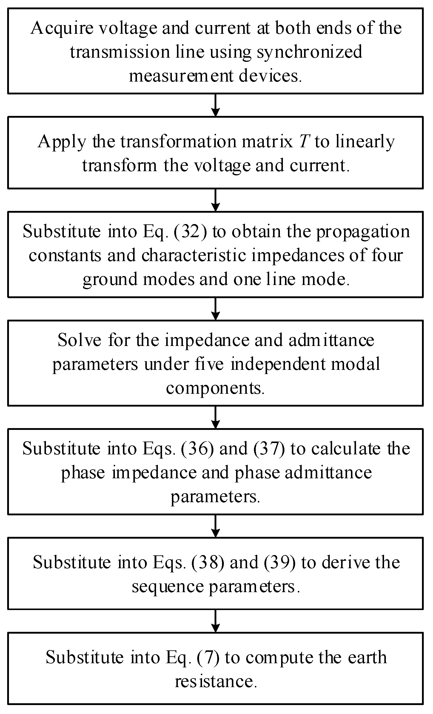
2.2. Distribution Parameter Measurement Method for Four-Circuit Parallel Lines with Same Voltage

In parameter measurement, ensuring accuracy requires the synchronization of signals at both ends of the four-circuit parallel line, so that the phase angle deviation remains within an acceptable range. This can be achieved using timing systems such as GPS or the BeiDou satellite system.

Since the ground mode and line mode correspond to the zero-sequence and positive-sequence parameters, respectively, it is necessary to generate both positive-sequence and zero-sequence signals for measurement. Common line parameter measurement methods are generally classified into two categories: de-energized measurement and live-line measurement. The method proposed in this paper is applicable to both de-energized and live-line operation scenarios. Below is a description of the parameter measurement method in the non-full-phase operation scenario of the line:

When the line is in a non-full-phase operating state, synchronized measurement devices such as PMUs at both ends of the line are used to synchronously collect the voltage and current of each phase of the line. The transformation matrix $T$ is then used to linearly transform the voltage and current of the twelve-phase system of the four-circuit line, obtaining the independent four ground modes and one line mode at the start and end of the line. Taking the ground mode $G_1$ as an example, after obtaining the modal parameters of the start and end voltages and currents, these can be substituted into Equation (32), allowing the propagation constant ${\gamma }_1$ and characteristic impedance $Z_{C\left(G1\right)}$ under the mode $G_1$ to be solved as follows:

$$\left\{\begin{array}{l}{\gamma }_1={\displaystyle \frac{1}{l}}\mathrm{arcosh}\left({\displaystyle \frac{{\dot{U}}_{10}{\dot{I}}_{10}+{\dot{U}}_{1r}{\dot{I}}_{1r}}{{\dot{U}}_{10}{\dot{I}}_{1r}+{\dot{I}}_{10}{\dot{U}}_{1r}}}\right)\\ Z_{C\left(G1\right)}={\displaystyle \frac{{\dot{U}}_{10}-{\dot{U}}_{1r}\cosh \left({\gamma }_{1}l\right)}{{\dot{I}}_{1r}\sinh \left({\gamma }_{1}l\right)}}\end{array}\right.$$

(33)

Since $Z_{C\left(G1\right)}=Z_{G1}\cdot {\gamma }_1^{-1}$, the impedance $Z_{G1}$ under the ground mode $G_1$, is given by:

$$Z_{G1}=Z_{C\left(G1\right)}\cdot {\gamma }_1$$

(34)

The admittance $Y_{G1}$ under the ground mode $G_1$ is:

$$Y_{G1}={\displaystyle \frac{{\gamma }_1^2}{Z_{G1}}}={\displaystyle \frac{{\gamma }_1}{Z_{C\left(G1\right)}}}$$

(35)

After obtaining the impedance and admittance parameters under the ground mode $G_1$, the same method can be applied to solve for the impedance and admittance parameters under the other four independent modes. Once the impedance and admittance parameters under all modes are solved, substitute them into Equations (21) and (22) to obtain all phase impedance and phase admittance parameters, with the calculation formulas as shown in Equations (36) and (37):

$$\left[\begin{array}{c}{Z}_s\\ Z_m\\ Z_{m1}\\ Z_{m2}\\ Z_{m3}\end{array}\right]={\left[\begin{array}{ccccc}1& 2& 3& 3& 3\\ 1& 2& 3& -3& -3\\ 1& 2& -3& 3& -3\\ 1& 2& -3& -3& 3\\ 1& -1& 0& 0& 0\end{array}\right]}^{-1}\left[\begin{array}{c}{Z}_{G1}\\ Z_{G2}\\ Z_{G3}\\ Z_{G4}\\ Z_{L1}\end{array}\right]$$

(36)

$$\left[\begin{array}{c}{Y}_s\\ Y_m\\ Y_{m1}\\ Y_{m2}\\ Y_{m3}\end{array}\right]={\left[\begin{array}{ccccc}1& 2& 3& 3& 3\\ 1& 2& 3& -3& -3\\ 1& 2& -3& 3& -3\\ 1& 2& -3& -3& 3\\ 1& -1& 0& 0& 0\end{array}\right]}^{-1}\left[\begin{array}{c}{Y}_{G1}\\ Y_{G2}\\ Y_{G3}\\ Y_{G4}\\ Y_{L1}\end{array}\right]$$

(37)

After solving for all the phase parameters, the symmetric component method can be used to obtain all the sequence parameters for the four-circuit line. Due to the unique symmetry of the line parameters, each sequence parameter can be directly given by the following equations:

$$\left\{\begin{array}{l}{Z}_1=Z_s-Z_m=R_1+j\omega L_1\\ Z_0=Z_s+2Z_m=R_0+j\omega L_0\\ Z_{012}=3Z_{m1}=R_{012}+j\omega L_{012}\\ Z_{013}=3Z_{m2}=R_{013}+j\omega L_{013}\\ Z_{014}=3Z_{m3}=R_{014}+j\omega L_{014}\end{array}\right.$$

(38)

$$\left\{\begin{array}{l}{Y}_1=Y_s-Y_m=j\omega C_1\\ Y_0=Y_s+2Y_m=j\omega C_0\\ Y_{012}=3Y_{m1}=j\omega C_{012}\\ Y_{013}=3Y_{m2}=j\omega C_{013}\\ Y_{014}=3Y_{m3}=j\omega C_{014}\end{array}\right.$$

(39)

where $R_1$, $L_1$, and $C_1$ are the positive-sequence self-resistance, self-inductance, and self-capacitance per unit length of a single circuit line, respectively; $R_0$, $L_0$, and $C_0$ are the zero-sequence self-resistance, self-inductance, and self-capacitance per unit length of a single circuit line, respectively; $R_{012}$, $L_{012}$, and $C_{012}$ are the zero-sequence mutual resistance, mutual inductance, and mutual capacitance per unit length between line 1 and line 2, respectively; $R_{013}$, $L_{013}$, and $C_{013}$ are the zero-sequence mutual resistance, mutual inductance, and mutual capacitance per unit length between line 1 and line 3, respectively; and $R_{014}$, $L_{014}$, and $C_{014}$ are the zero-sequence mutual resistance, mutual inductance, and mutual capacitance per unit length between line 1 and line 4, respectively.

Once all zero-sequence and positive-sequence parameters are obtained, the ground resistance value of the four-circuit parallel line can be calculated using Equation (7). Therefore, in addition to the calculations for the ground resistance, there are a total of 16 parameters to be measured for the four-circuit parallel line.

The measurement process of transmission line distributed parameters is illustrated in Figure 3.

3. Simulation Example Analysis

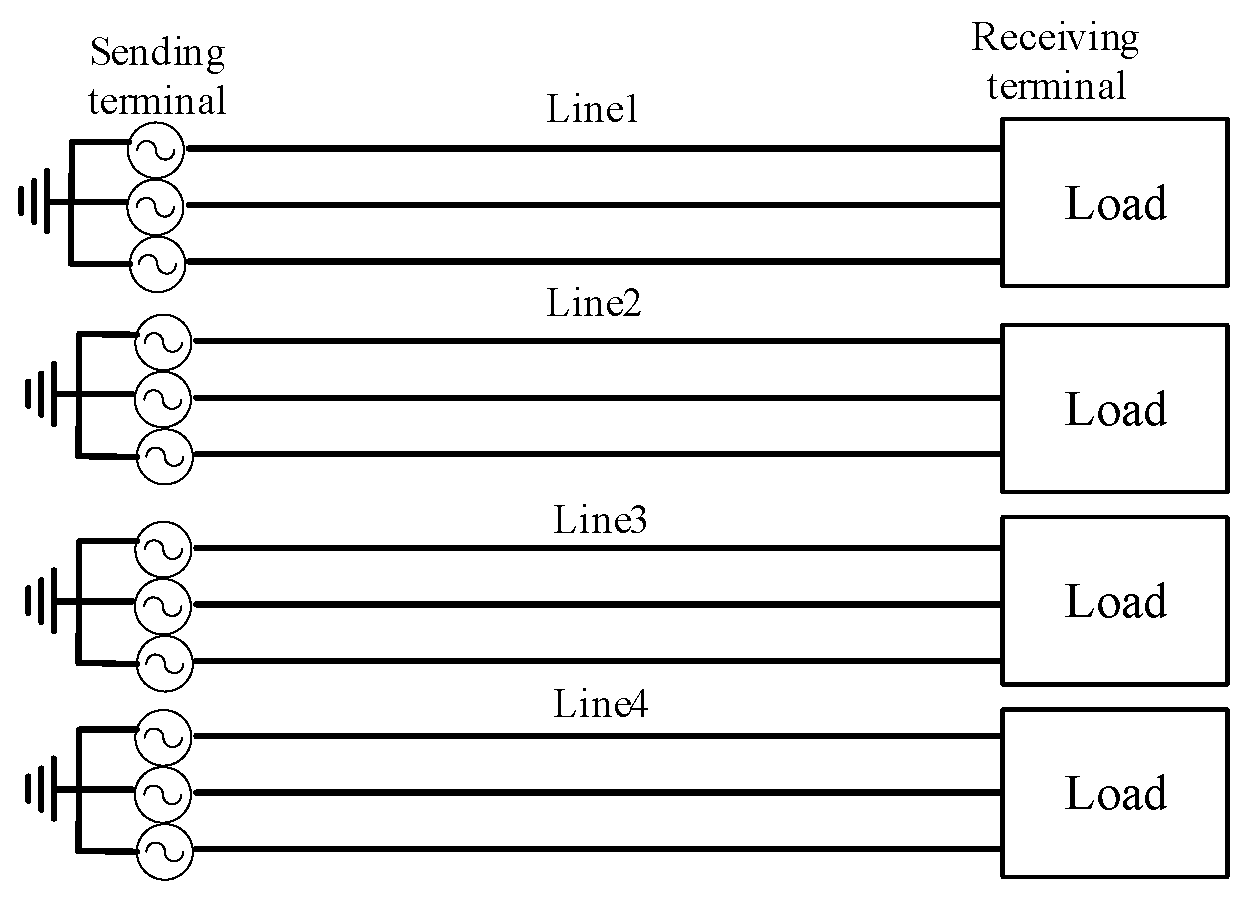
3.1. PSCAD Simulation Model of Four-Circuit Parallel Lines with Same Voltage Level

In this simulation, the four-circuit transmission line is modeled using a distributed parameter model, which effectively captures the spatial variations in voltage and current along the line. The transmission line equations are derived from Maxwell’s equations and solved using the phase-mode transformation method to facilitate accurate parameter estimation.

To ensure a stable reference for parameter extraction, the voltage source in the simulation model is represented by an ideal three-phase balanced source operating at a fixed frequency of 50 Hz. The simulation model is implemented in PSCAD, as illustrated in Figure 4, with a sampling frequency of 4000 Hz and a total simulation time of 1 s. The soil resistivity along the line is set to $\rho =80.8\mathrm{\Omega }\cdot m$.

The theoretical parameter values of the four-circuit parallel line are shown in

Table 1. Line theoretical parameter values of the four-circuit lines at the same voltage level.

R0 (Ω/km)	R012 (Ω/km)	R013 (Ω/km)	R014 (Ω/km)	R1 (Ω/km)
0.1686	0.1577	0.1553	0.1553	0.0110
L0 (mH/km)	L012 (mH/km)	L013 (mH/km)	L014 (mH/km)	L1 (mH/km)
2.6620	1.7903	1.5366	1.4737	0.6975
C0 (nF/km)	C012 (nF/km)	C013 (nF/km)	C014 (nF/km)	C1 (nF/km)
rg (Ω/km)
0.0525

.

In this study, the measurement error is evaluated by comparing the estimated transmission line parameters with the theoretical values set in the simulation model. The measurement error calculation formula used in this paper is defined as:

$$\mathrm{error}=\left|{\displaystyle \frac{x-x_0}{x_0}}\right|\times 100\%$$

(40)

where $x$ is the parameter calculated from the simulation, and $x_0$ is the reference value, where the reference value corresponds to the predefined transmission line parameters in the PSCAD simulation model. This approach ensures a consistent and objective evaluation of the proposed method under controlled conditions.

3.2. Simulation Analysis of the Proposed Method

3.2.1. Investigating the Effect of Line Length on the Measurement Accuracy of the Proposed Method

With all other conditions constant, the total length of the line $l$ is varied. The simulation results are shown in

Table 2. Line inductance measurement results using the proposed method.

Line Length (km)		50	100	200	300	400	500
rg	Measurement Error (%)	0.9832	0.9243	0.6607	0.6237	0.9210	0.9267
R0	Measurement Error (%)	1.0717	0.9465	0.7037	0.6465	0.8483	0.8851
R012	Measurement Error (%)	1.0534	1.2822	0.7536	0.7475	1.2784	0.9763
R013	Measurement Error (%)	1.1404	1.1858	0.7580	0.7875	1.1163	0.9638
R014	Measurement Error (%)	1.1333	1.1098	0.7606	0.7778	1.0164	0.9480
R1	Measurement Error (%)	2.3387	1.2644	1.3189	0.9719	0.1923	0.2896
L0	Measurement Error (%)	0.1189	0.1888	0.1806	0.1275	0.1102	0.1291
L012	Measurement Error (%)	0.1889	0.2334	0.2692	0.1964	0.1811	0.1887
L013	Measurement Error (%)	0.2489	0.2871	0.3288	0.2437	0.2233	0.2369
L014	Measurement Error (%)	0.2620	0.2967	0.3400	0.2566	0.2280	0.2464
L1	Measurement Error (%)	0.0724	0.0241	0.0117	0.0417	0.0915	0.0280
C0	Measurement Error (%)	2.7997	1.7436	0.0591	0.1694	0.0395	0.0024
C012	Measurement Error (%)	0.2931	0.7778	0.1861	0.0151	0.0389	0.0938
C013	Measurement Error (%)	3.1217	1.8721	0.3754	0.0322	0.0837	0.0444
C014	Measurement Error (%)	0.3105	2.1407	1.3148	0.3791	0.1255	0.1834
C1	Measurement Error (%)	2.1929	1.6372	0.4876	0.7867	0.7181	0.6259

.

From Table 2, it can be observed that as the length of the four-circuit line increases, the measurement results for each parameter using the proposed method maintain high accuracy. This demonstrates that the method overcomes the distribution effect of long lines, and the measurement results do not significantly change with an increase in line length.

Investigating the Effect of Theoretical Parameter Values on the Measurement Accuracy of the Proposed Method. Transmission lines at different voltage levels have varying conductor materials, number of split conductors, split radii, and tower structures, which result in different theoretical parameter values. Therefore, it is important to verify the robustness of the proposed method by changing the theoretical parameter values of the overhead line.

The line length is fixed at 300 km, and the simulation results of the proposed method are shown in Figure 5.

The errors shown in Figure 5 represent the maximum measurement errors for each sequence of resistance, inductance, and capacitance. From Figure 5, it can be concluded that the proposed method exhibits high measurement accuracy for all resistance, inductance, and capacitance parameters. The measurement errors for inductance and capacitance are all below 1%, while the resistance parameters, which show more fluctuation, have measurement errors within 1.8%. Therefore, the proposed measurement method is suitable for the parameter measurement of transmission lines at any voltage level.

In actual on-site measurements, a test power source and specialized measuring instruments are required for the measurement. The measuring instruments are capable of synchronously collecting voltage and current signals and saving the data. Meanwhile, current and voltage need to be collected from the current and potential transformers of the transmission line. When the test signal is too weak, the collected voltage and current may be distorted. Next, the impact of voltage and current distortion rates on the measurement results will be analyzed. The maximum deviation caused in the measurement results is shown in Figure 6.

The above results demonstrate that even minor distortions in voltage and current can significantly impact the measurement results, leading to considerable deviations from the original values. When the test power source output is insufficient, severe distortions may occur in the signals acquired from the current and potential transformers. In actual on-site measurements, the influence of these transformers must be carefully considered. In particular, special attention should be paid to the accuracy of the collected voltage and current signals, as such distortions can cause measurement errors exceeding 8%.

Next, an analysis is conducted on the impact of changes in the grounding resistance along the line, which are caused by variations in soil resistivity or seasonal fluctuations, on the measurement results. To assess this impact, a deviation is introduced to the grounding resistance, and its influence on the measurement results is analyzed. The results are presented in Figure 7.

Although factors such as conductor heating, glaze, corona discharge, and humidity may cause variations in ground resistance, the proposed method exhibits strong adaptability to these changes. As a result, the measurement error remains consistently within 3%.

In practical measurements, precise synchronization of voltage and current measurements at both ends of the transmission line is essential for ensuring measurement accuracy. High-precision synchronization is typically maintained using the Global Positioning System (GPS) or BeiDou Timing System. However, synchronization errors may still arise due to factors such as timing deviations in measurement devices, signal transmission delays, and environmental interference. To quantitatively evaluate the influence of synchronization errors, a time offset $\mathrm{\Delta }t$ is introduced between the measurement signals at the sending and receiving ends of the transmission line, and its effect on parameter estimation is analyzed. The simulation results are shown in

Table 3. Measurement errors under Different Synchronization Deviations.

$$\mathbf{\Delta }\mathit{t}(\mathit{\mu }\mathit{s})$$	0	50	100	150	200
R (%)	0.7220	1.4870	3.698	5.9090	8.1240
L (%)	0.5831	0.5715	1.7270	2.8850	4.0430
C (%)	0.8556	1.7620	4.3820	7.0040	9.6280

.

In practical measurements, a lack of synchronization between data acquisition systems at the sending and receiving ends of a transmission line can impact measurement accuracy. As synchronization errors increase, the estimation errors grow larger. However, systems like GPS or BeiDou typically provide reliable timing, minimizing these errors. In most engineering applications, such synchronization is sufficient to meet accuracy requirements, ensuring minimal impact on measurement precision.

3.2.2. Comparison of the Proposed Method with Other Methods

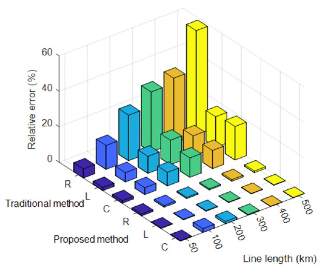
• Comparison with Traditional Methods

The traditional measurement method is a single-ended technique based on a concentrated parameter model. During measurement, it only requires the collection of voltage and current from one side of the line, without the need for synchronized two-end measurements. Moreover, each measurement can only calculate one impedance or admittance parameter of the line. Therefore, to determine all 16 parameters of the model proposed in this paper, a total of 10 independent measurements are required.

Table 4. Line parameter measurement error using the traditional method.

Line Length (km)		50	100	200	300	400	500
rg	Measurement Error (%)	5.1234	13.4567	25.6789	33.8901	36.7807	58.6987
R0	Measurement Error (%)	4.2345	11.5678	22.7890	30.9012	34.8272	55.5088
R012	Measurement Error (%)	4.3456	11.6789	23.0123	31.1234	34.7384	55.2544
R013	Measurement Error (%)	4.5678	12.8901	24.3456	32.4567	36.5562	58.3499
R014	Measurement Error (%)	4.6789	13.0123	24.6789	32.7890	36.5721	58.4843
R1	Measurement Error (%)	2.0123	6.3456	10.6789	14.8901	11.8627	17.2690
L0	Measurement Error (%)	1.7456	5.2345	9.5678	13.7890	11.3772	17.3043
L012	Measurement Error (%)	2.2567	6.1234	10.9012	15.0123	13.7779	21.0682
L013	Measurement Error (%)	2.4678	6.5678	11.3456	16.4567	15.4273	23.6507
L014	Measurement Error (%)	2.5789	6.8901	11.7890	16.8901	15.8255	24.2799
L1	Measurement Error (%)	1.0456	2.8901	5.3456	7.9012	5.4285	7.9759
C0	Measurement Error (%)	1.4567	3.9012	7.6789	10.9012	10.2419	18.8847
C012	Measurement Error (%)	2.0678	5.1234	9.7890	13.9012	14.0023	18.2471
C013	Measurement Error (%)	2.1789	5.4567	10.1234	14.3456	16.2844	23.6490
C014	Measurement Error (%)	2.1012	5.3456	9.9012	14.1234	15.4723	24.8934
C1	Measurement Error (%)	1.3678	3.4567	6.7890	9.5678	10.9535	18.0262

presents the results of using the traditional method to measure line parameters. A comparison of the results obtained from both methods is shown in Figure 8.

The data indicate that the traditional method not only involves complex measurement steps but also exhibits significant distribution effects in the measurement results. As the line length increases, the measurement errors for various parameters also grow. For long lines, such as those between 50 and 500 km, the error in measuring resistance parameters can exceed 50%, which is unacceptable for engineering applications. Therefore, the traditional method is not suitable for measuring the parameters of long transmission lines.

2.

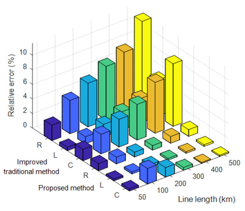
Comparison with the Improved Traditional Method

The principle of the improved traditional method is also based on the concentrated parameter model of the line, but it incorporates synchronous voltage and current measurements at both ends of the line. By averaging the current at both ends, this method indirectly accounts for the effect of distributed capacitance along the line. During measurement, the entire four-circuit line must be powered off, and measurements are conducted under five independent operational modes.

Table 5. Line resistance measurement results using the improved traditional method.

Line Length (km)		50	100	200	300	400	500
rg	Measurement Error (%)	2.1234	4.5678	5.9876	7.3456	8.3461	11.6332
R0	Measurement Error (%)	1.9876	4.2345	5.6789	6.9012	7.9876	11.1283
R012	Measurement Error (%)	2.1012	4.3456	5.8901	7.1234	8.3263	11.5668
R013	Measurement Error (%)	2.1012	4.3456	5.8901	7.1234	8.3263	11.5668
R014	Measurement Error (%)	2.1234	4.5678	5.9876	7.3456	8.3426	11.6916
R1	Measurement Error (%)	0.8765	1.9012	2.3456	3.0123	2.9459	3.9526
L0	Measurement Error (%)	0.3842	0.8265	1.4523	2.0156	2.4577	3.6330
L012	Measurement Error (%)	0.4637	0.9521	1.6849	2.4378	3.2565	4.8364
L013	Measurement Error (%)	0.4478	0.9134	1.6257	2.3019	3.2565	4.8364
L014	Measurement Error (%)	0.4765	0.9783	1.7132	2.4861	3.3282	4.9500
L1	Measurement Error (%)	0.3579	0.7426	1.2890	1.8643	2.2936	3.8602
C0	Measurement Error (%)	1.2345	2.3456	3.4567	4.5678	4.8935	6.3605
C012	Measurement Error (%)	1.5678	2.6789	3.7890	4.8901	6.9652	8.5748
C013	Measurement Error (%)	1.8901	2.9012	4.0123	5.1234	7.9518	9.2278
C014	Measurement Error (%)	1.3456	2.4567	3.5678	4.6789	4.9647	6.7766
C1	Measurement Error (%)	1.0123	2.1234	3.2345	4.3456	4.0147	5.1626

presents the measurement results obtained using the improved traditional method as the line length varies from 50 km to 500 km.

To compare the two methods, typical data for line lengths ranging from 50 km to 500 km are selected, and the measurement results of both methods are shown in Figure 9.

As illustrated in Figure 9, the proposed method consistently maintains high measurement accuracy across all line lengths, effectively overcoming the distribution effects of long lines. In contrast, the improved traditional method, which relies on the concentrated parameter model, does not fully account for the variations in voltage and current along the line. As a result, the measurement errors increase with the line length.

3.3. Discussion and Prospect

This section summarizes the key findings from the simulation analysis and discusses the implications, practical challenges, and assumptions of the proposed method.

3.3.1. Discussion of Results

• High Measurement Accuracy. The proposed distributed parameter measurement method maintains high accuracy across different transmission line lengths. Unlike traditional methods, which rely on single-ended measurements and neglect distributed effects, this approach incorporates the full transmission equation and phase-mode transformation, ensuring precise parameter extraction. The measurement errors remain below 2% for resistance, inductance, and capacitance, representing a significant improvement over conventional methods.
• Improved Performance Compared to Traditional Methods. The proposed method provides a cost-effective and practical solution for measuring the distributed parameters of four-circuit transmission lines. It achieves high accuracy and reliability by fully considering the distributed characteristics of transmission lines, unlike traditional methods that rely on lumped parameter models and exhibit increasing errors with longer line lengths. Additionally, the proposed method requires only a single measurement for full parameter estimation, significantly enhancing efficiency compared to traditional methods (requiring 10 measurements) and improved methods (requiring 5 measurements). It utilizes standard measurement devices such as voltage and current transformers, data acquisition systems, and GPS/BeiDou receivers, eliminating the need for specialized equipment and complex calibration procedures.
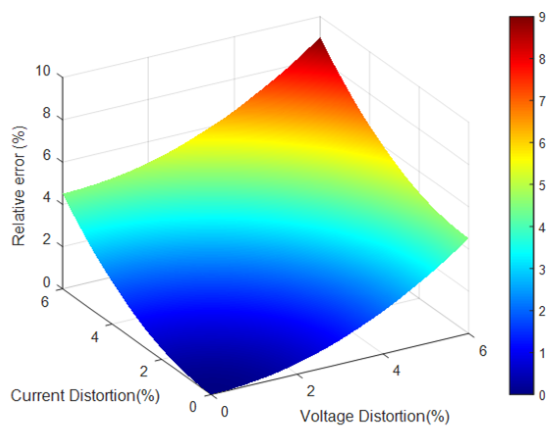
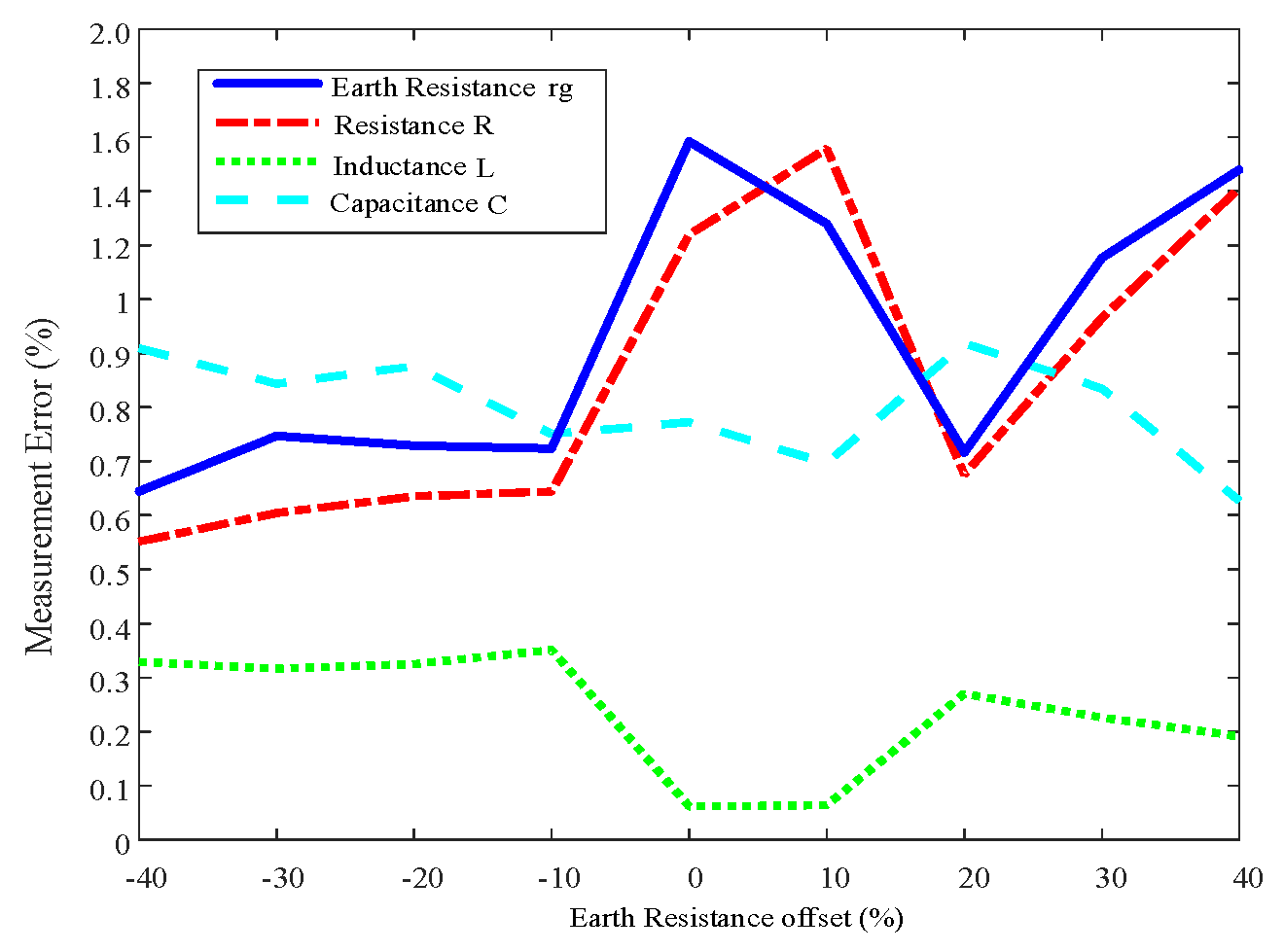
• Practical Applicability and Challenges. Although the proposed method has been validated through simulations, real-world implementation may present challenges. Factors such as external disturbances, environmental conditions, and equipment inaccuracies can affect measurement accuracy. Furthermore, precise synchronization of measurements at both ends of the line is necessary, which can be achieved using GPS or BeiDou satellite systems. The method also demonstrates strong adaptability to variations in ground resistance parameters, maintaining high testing accuracy. Future research should explore advanced filtering techniques and error compensation models to enhance robustness under practical conditions.

3.3.2. Assumptions and Limitations

• Ideal Measurement Conditions. The method assumes minimal external interference and uniform soil resistivity along the transmission line. However, it does not fully account for the complex electromagnetic interference that may occur in field measurements, which could introduce additional uncertainties. In practice, variations in soil conditions and electromagnetic disturbances may introduce measurement uncertainties.
• Simulation-Based Validation. The evaluation of the proposed method is primarily based on simulations. While the results confirm theoretical effectiveness, real-world applications may encounter additional issues such as sensor calibration errors, signal distortion, and operational constraints.
• Influence of Environmental Factors. The method’s performance may be affected by environmental factors such as glaze accumulation, humidity, and extreme weather conditions. These effects were not fully modeled in the simulations, and future work should consider integrating adaptive compensation techniques to mitigate their impact.

4. Conclusions

This paper presents a precise measurement method for the distributed parameters of four parallel transmission lines under the same voltage, explicitly considering ground resistance. The proposed method is derived based on the phase transformation principle and distributed parameter model, utilizing the full transmission equation without approximations. Its accuracy and efficiency have been validated through theoretical analysis and digital simulations, and its performance has been compared with traditional and improved traditional methods. The key conclusions are summarized as follows:

• The proposed method can simultaneously measure all 16 distributed parameters of four parallel transmission lines under the same voltage, including ground resistance. This ensures a more comprehensive and precise parameter extraction compared to traditional methods.
• By incorporating the full transmission equation and phase transformation, the proposed method eliminates approximation errors, maintaining high accuracy across different transmission line lengths and voltage levels.
• Traditional measurement approaches rely on single-ended data and approximate the other end, leading to accuracy degradation, especially for long lines. The proposed method fully considers distributed effects along the line, significantly improving reliability.
• The method requires only a single measurement to obtain all distributed parameters, whether the line is de-energized or energized. In contrast, traditional and improved methods require 10 and 5 independent measurements, respectively, making the proposed approach much more efficient.
• The proposed method is suitable for both de-energized and energized transmission lines, making it adaptable to a wide range of practical applications in power system operation and maintenance.
• While the method has been validated through simulations, practical deployment may face challenges such as measurement synchronization, environmental influences, and equipment calibration. Future work should focus on real-world verification and improving robustness under operational conditions.

References

1. Yuan, K.; Zhang, T.; Xie, X.; Du, S.; Xue, X.; Abdul-Manan, A.F.N.; Huang, Z. Exploration of Low-Cost Green Transition Opportunities for China’s Power System Under Dual Carbon Goals. J. Clean. Prod. 2023, 414, 137590. [Google Scholar] [CrossRef]
2. Liu, S.; Lin, Z.; Jiang, Y.; Zhang, T.; Yang, L.; Tan, W.; Lu, F. Modelling and Discussion on Emission Reduction Transformation Path of China’s Electric Power Industry Under “Double Carbon” Goal. Heliyon 2022, 8, e10497. [Google Scholar] [CrossRef] [PubMed]
3. Li, Z.; Xia, Y.; Luo, Y.; Xiong, J. Research on the Development of a New Power System Under the “Dual Carbon” Goals. In Proceedings of the 2024 Boao New Power System International Forum—Power System and New Energy Technology Innovation Forum (NPSIF), Boao, China, 8–10 December 2024; pp. 758–762. [Google Scholar]
4. Tong, J.; Liu, W.; Mao, J.; Ying, M. Role and Development of Thermal Power Units in New Power Systems. IEEE J. Radio Freq. Identif. 2022, 6, 837–841. [Google Scholar] [CrossRef]
5. Song, Y.; Yang, S.; Li, H. Research on Transmission Scheme of Large-Scale Renewable Energy Transmitted Through Series Hybrid DC System. In Proceedings of the 2022 IEEE 6th Conference on Energy Internet and Energy System Integration (EI2), Chengdu, China, 11–13 November 2022; pp. 363–368. [Google Scholar]
6. Tong, D.; Farnham, D.J.; Duan, L.; Zhang, Q.; Lewis, N.S.; Caldeira, K.; Davis, S.J. Geophysical Constraints on the Reliability of Solar and Wind Power Worldwide. Nat. Commun. 2021, 12, 6146. [Google Scholar] [CrossRef] [PubMed]
7. Luo, J.; Liu, Y.; Cui, Q.; Zhong, J.; Zhang, L. Single-Ended Time Domain Fault Location Based on Transient Signal Measurements of Transmission Lines. Prot. Control Mod. Power Syst. 2024, 9, 61–74. [Google Scholar] [CrossRef]
8. Panahi, H.; Zamani, R.; Sanaye-Pasand, M.; Mehrjerdi, H. Advances in Transmission Network Fault Location in Modern Power Systems: Review, Outlook and Future Works. IEEE Access 2021, 9, 158599–158615. [Google Scholar] [CrossRef]
9. Liu, Y.; Wang, B.; Zheng, X.; Lu, D.; Fu, M.; Tai, N. Fault Location Algorithm for Non-Homogeneous Transmission Lines Considering Line Asymmetry. IEEE Trans. Power Deliv. 2020, 35, 2425–2437. [Google Scholar] [CrossRef]
10. Feng, X.; Qi, L.; Pan, J. A Novel Fault Location Method and Algorithm for DC Distribution Protection. IEEE Trans. Ind. Appl. 2017, 53, 1834–1840. [Google Scholar] [CrossRef]
11. Liang, J.; Jing, T.; Niu, H.; Wang, J. Two-Terminal Fault Location Method of Distribution Network Based on Adaptive Convolution Neural Network. IEEE Access 2020, 8, 54035–54043. [Google Scholar] [CrossRef]
12. Peng, Z.; Zhang, W.; Chen, P.; Gong, X.; Wang, L.; Liu, F. Model and Unbalance Analysis of Double-Circuit Transmission Lines on the Same Tower. In Proceedings of the 2022 IEEE 2nd International Conference on Electronic Technology, Communication and Information (ICETCI), Changchun, China, 27–29 May 2022; pp. 65–69. [Google Scholar]
13. Hu, Z.; Xiong, M.; Li, C.; Tang, P. New Approach for Precisely Measuring the Zero-Sequence Parameters of Long-Distance Double-Circuit Transmission Lines. IEEE Trans. Power Deliv. 2016, 31, 1627–1635. [Google Scholar] [CrossRef]
14. Liang, Y.; Guo, J.; Wang, G. Parameter Self-Adaptive Fault Location of Four-Parallel Transmission Lines on the Same Tower. In Proceedings of the 2011 4th International Conference on Electric Utility Deregulation and Restructuring and Power Technologies (DRPT), Weihai, China, 6–9 July 2011; pp. 881–884. [Google Scholar]
15. Sima, W.; Wang, R.; Yang, M.; Yang, Q.; Yuan, T. Secondary Arc Current of Ultra-High Voltage Transmission Line with a Mixed Voltage of 1000/500 kV on a Single Tower. IET Gener. Transm. Distrib. 2015, 9, 686–693. [Google Scholar] [CrossRef]
16. Hu, Z.; Chen, Y. New Method of Live Line Measuring the Inductance Parameters of Transmission Lines Based on GPS Technology. IEEE Trans. Power Deliv. 2008, 23, 1288–1295. [Google Scholar] [CrossRef]
17. Tan, B.; Dong, X.; Liu, M.; Bi, S.; Yang, J.; Tong, X.; Wang, X. Configuration Method and Test Verification for Equalizing Resistance of HVDC Earth Electrode Considering Anisotropy of Soil Resistivity Distribution. High Volt. Appar. 2021, 57, 0144–0150. [Google Scholar] [CrossRef]
18. Dong, Q.; Shao, P. Error analysis and improvement measures of single-phase power supply method to measure the impedance parameters of single-circuit asymmetric line. Electr. Meas. Instrum. 2018, 55, 15–19+30. [Google Scholar] [CrossRef]
19. Apostolopoulos, C.A.; Korres, G.N. A Novel Fault-Location Algorithm for Double-Circuit Transmission Lines Without Utilizing Line Parameters. IEEE Trans. Power Deliv. 2011, 26, 1467–1478. [Google Scholar] [CrossRef]
20. Xiao, Y.; Deng, J.; Xia, G.; Yang, X.; Zhang, J. A Novel Distributed Parameters Measurement Method of HVDC Transmission Line. Proc. CSEE 2015, 35, 5375–5383. [Google Scholar] [CrossRef]
21. Xiao, Y.; Fan, Y.; Cheng, L.; Deng, J. A Parameter Measurement Theory of Single and Double Circuit AC Transmission Lines. Proc. CSEE 2016, 36, 5515–5522+5727. [Google Scholar] [CrossRef]
22. Xiao, Y.; Deng, J.; Fan, Y.; Cheng, L. Decoupling Measurement of Zero Sequence Parameters for Four-Circuit AC Transmission Lines on Same Tower. South. Power Syst. Technol. 2016, 10, 54–59. [Google Scholar] [CrossRef]
23. Yan, T.; Tan, Y.; Li, H.; Gao, M.; Hu, Z. Anti-Interference Measurement Method of Zero Sequence Capacitance of Transmission Lines Based on Harmonic Component. In Proceedings of the 2022 4th Asia Energy and Electrical Engineering Symposium (AEEES), Chengdu, China, 25–28 March 2022; pp. 674–679. [Google Scholar]
Figure 1. Physical model of the three-phase line considering ground return effects.
Energies 18 01805 g001
Figure 2. Physical model of the four-circuit line on the same tower.
Energies 18 01805 g002
Figure 3. Flowchart of transmission line distributed parameter measurement.
Energies 18 01805 g003
Figure 4. PSCAD simulation model of the four-circuit line at the same voltage level.
Energies 18 01805 g004
Figure 5. Measurement errors of the proposed method as a function of theoretical parameter values.
Energies 18 01805 g005
Figure 6. The impact of voltage and current distortion rates on the measurement results.
Energies 18 01805 g006
Figure 7. Influence of grounding resistance variation on measurement results.
Energies 18 01805 g007
Figure 8. Error comparison between the proposed method and the traditional method.
Energies 18 01805 g008
Figure 9. Error comparison between the proposed method and the improved traditional method.
Energies 18 01805 g009