The Impact of Energy Intensity, Renewable Energy, and Financial Development on Green Growth in OECD Countries: Fresh Evidence Under Environmental Policy Stringency

Abstract

This study examines the impact of financial development, renewable energy, energy intensity, and stringent environmental policies on green growth in twenty-three Organization for Economic Cooperation and Development countries from 2000 to 2023. Additionally, it examines how stringent environmental policies moderate the link between financial development and green growth. Economic complexity, trade openness, and green technology variables are also included in the model as control variables. The index is constructed using economic growth, education, health, CO₂ emissions, net forest, and mineral components for green growth, the main variable explained in the research. The Fully Modified Ordinary Least Squares method is applied to estimate elasticity coefficients in the study. The findings show that financial development and energy intensity have a negative impact on green growth, whereas strict environmental policies and renewable energy support green growth. Moreover, the interaction between financial development and stringent environmental policies promotes green growth. At the same time, the control variables of trade openness and economic complexity have a negative impact on green growth, while green technology makes a positive contribution. Furthermore, financial development and energy intensity have the most significant quantitative impact on green growth, while trade openness and stringent environmental policies have the least impact. In line with these findings, environmentally friendly financial instruments and green investments should be supported instead of directing financial resources only to industry-intensive sectors in Organization for Economic Cooperation and Development countries. In this context, implementing energy efficiency policies and increasing incentives for renewable energy are of great importance.

1. Introduction

The accelerating pace of climate change has made it more challenging to balance economic growth and environmental damage, increasing the need for policymaking in this direction. Therefore, combating climate change should not be limited to local environmental issues such as water and air quality, but should be treated as a global priority. Accordingly, green growth policies provide an essential framework for achieving sustainable development goals [1]. In its Towards Green Growth report, the OECD defines green growth as promoting economic growth and development while preserving the sustainability of natural resources and environmental services. To achieve this, investments and innovations that support sustainable growth should be encouraged, and new economic opportunities should be created [2].

The green growth concept is widely accepted globally, and a shared understanding is being established among countries and organizations to use resources more efficiently, ensure environmental sustainability, and increase resilience. Regardless of economic development level, institutional structures and systematic policy design play an essential role in achieving green growth; this is also true for countries in the development process [3]. Green growth theory is an approach adopted by national and international policies and supported by multilateral organizations. It assumes that GDP growth can be fully decoupled from resource use and carbon emissions, and that this process can occur at a pace that prevents ecological degradation and climate change [4].

Green growth is a promising approach that offers solutions to current global challenges by balancing economic progress with environmental protection [5]. For this theory to be effectively implemented, economic development must be balanced with environmental sustainability. Financial development is critical here, stimulating capital accumulation and technological progress, thus supporting environmentally friendly investments and innovations. This process leads to increased savings and investment rates, effective management of foreign capital inflows, and sustainable economic growth. Especially in emerging economies, financial development is recognized as a powerful economic driver [6].

Simultaneously, financial development stands out as one of the key elements of green growth. Nations with more developed financial systems invest more in environmentally friendly technologies and policies. The reason is that financial institutions offer the necessary financing for green projects and support sustainable development by ensuring the efficient allocation of resources. Accordingly, financial development’s capital flows and investment opportunities contribute to achieving environmental sustainability goals [7]. However, the credit market can affect economic and environmental factors through positive or negative effects on firms, leading to fluctuations in related indicators [8]. However, it is observed in the literature that the impact of financial development on green growth differs according to the level of development of countries [3,9]. Therefore, consensus on the effect of financial development on green growth is still lacking.

Conversely, one of the main challenges in achieving green economic growth is energy resources. Today, energy is seen not only as a component of the production process but also as a means of power, influence, and diplomatic impact on a global scale. Non-renewable sources account for a larger share of energy consumption worldwide than clean energy [10]. Using clean energy sources is directly linked to sustainable economic development because production processes using renewable energy sources such as geothermal, solar, biomass, hydro, and wind minimize environmental externalities. This contributes to preserving natural capital stocks while ensuring the sustainability of renewable energy production. Ending the use of coal in the energy mix, controlling deforestation, expanding the use of electric vehicles, and investing in sources of renewable energy are essential for achieving sustainable development goals and green growth [11,12].

Reducing environmental pollution is a critical goal for sustainable development; however, environmental pollution emerges as a negative externality of economic activities. Since market mechanisms alone cannot correct this imbalance, governments must intervene through environmental policies and regulations. Strict environmental rules encourage individuals and businesses to limit pollution emissions, while ensuring effective government participation in environmental governance [13]. However, while stringent environmental policies promote green innovation, their effectiveness cannot be determined without incentive mechanisms. Strict environmental policies aim to transform society’s lifestyle, production habits, and consumption towards a sustainable environment by increasing the cost of climate and pollution-related services [14]. Moreover, stringent environmental policies significantly affect financial markets in terms of both costs and opportunities. While strict regulations can limit profitability and investment by imposing additional financial burdens on businesses, they can also support the development of green finance by encouraging innovation. The ecological modernization approach suggests these policies can create a more sustainable and resilient economic structure. The rise of green bonds and sustainability-linked financial instruments shows that environmental factors are increasingly considered in financial decision-making [15].

Based on the above discussion, the current study seeks to answer the following questions in high-income OECD countries: (1) How do renewable energy use, energy intensity, and financial development affect green growth in OECD countries? (2) What are the implications of the interaction between environmental policy stringency and financial development for green growth? As advanced economies, OECD countries stand out with their high-income levels, robust institutional structures, and strong data systems [16]. On the other hand, in its report titled “Trust in Global Cooperation–The Vision for the OECD for the Next Decade”, the OECD commits to supporting countries in achieving a just transition to net-zero GHG emissions, prioritizing climate resilience and energy transition. To this end, it commits to helping OECD members achieve the 2015 Paris Agreement targets. In addition, in line with the 2030 Agenda for Sustainable Development, it aims to partner with developing countries to address sustainable development challenges and create standards. This approach seeks to ensure that the OECD’s overall policies are aligned with the OECD convention to promote global prosperity [17].

The current study provides various contributions to the literature. First, the effects of financial development on green growth remain unclear in the literature. While some studies [3,6,18] suggest that financial development will increase environmental sustainability and green growth by encouraging green investments, others [9] argue that financial resources can increase energy consumption in fossil energy-intensive industries. The OECD aims to align all financing flows with low greenhouse gas (GHG) emissions and climate-resilient development. It also aims to contribute to the financial system’s achievement of climate goals through government-backed international standards, best practice guidelines, and comprehensive policy recommendations, in cooperation with developed, emerging, and developing economies [19]. In this context, re-examining the ambiguous relationships between green growth and financial development in OECD countries is essential to evaluate the effectiveness of sustainable development policies and understand how the financial system drives green investments.

Second, explores how stringent environmental policies influence the linkage between green growth and financial development as a moderating factor. The OECD encourages implementing and formulating comprehensive environmental policies so that member countries can effectively deal with environmental challenges. Moreover, stringent environmental policies can have decisive effects on financial markets in terms of both additional financial burdens and new opportunities [15]. In this regard, we will assess how the interaction of stringent environmental policies with financial development can promote green growth and provide a new perspective on sustainable development. Third, the study focuses on the effects of energy intensity and renewable energy on green growth. Thus, the impact of energy efficiency policies on green growth will be evaluated, and the effect of these variables on green growth will be considered, providing a holistic perspective for sustainable development policies.

2. Literature Review and Hypothesis Development

The study focuses on the effects of renewable energy, financial development, energy intensity, and stringent environmental policies on green growth and considers their interaction. This section presents theoretical discussion, empirical findings, and research hypotheses on the effect of these variables on green growth.

2.1. Financial Development and Green Growth

The financial system’s efficient functioning and sound structure play a key role in the economic development of countries. In this context, the impact of financial development (FD) on economic growth is a frequently discussed topic in the literature with different variables and scopes [20,21]. However, there is no clear consensus on the direction and magnitude of this effect. While some studies suggest that financial development is a driving force that supports and improves the economy [22], other studies suggest that it may cause environmental damage despite its contribution to economic growth [23].

Therefore, the areas to which countries direct financial resources are of great importance. Suppose financial resources are channeled to fossil fuel-intensive sectors by focusing only on economic growth. In that case, energy consumption may increase, leading to environmental problems like air pollution. In this framework, using financial resources in the fossil energy industry may negatively affect sustainable growth [24]. On the other hand, if financial resources are used efficiently without ignoring environmental factors, purchasing energy-efficient, environmentally friendly machinery and equipment can be encouraged, and resources can be allocated to sustainable projects. In this case, using financial resources in renewable energy investments will contribute positively to sustainable growth by minimizing environmental damage [25].

In addition, increasing savings rates through a developed financial system, strengthening the depth of financial markets, directing foreign investments to environmentally friendly projects, and encouraging green investments by both the public and private sectors will play a critical role in supporting sustainable growth. As a result, countries’ capital accumulation, the level of development, the efficient functioning of their financial markets, and the level of financial development are among the determining factors in ensuring sustainable economic growth [26].

However, a noticeable gap exists in the literature regarding the effects of financial development (FD) on green growth (GG). In this respect, Ngo et al. [6], who examined the bidirectional connection between FD and GG across 36 developing and developed countries from 1996 to 2014, reported that both variables positively influence each other. Notably, the positive effect of FD on GG was found to be stronger than the reverse. This result is attributed to human capital, education expenditure, sustainable infrastructure financing, and energy efficiency. Similarly, Ahmed et al. [18], focusing on South Asian countries from 2000 to 2018, demonstrated that FD positively affects GG. With enhanced financial development, access to environmentally friendly machinery in the industry increases, contributing to improved environmental quality.

Yang et al. [27], in an analysis covering South Asian countries between 1990 and 2021, also confirmed a positive effect of FD on GG in the long and short run. Their findings indicate that the functioning of free markets helps reduce carbon emissions, while green technologies positively contribute to economic growth. In line with these results, Saqib et al. [3] showed that FD positively influences GG in the nations with the highest ecological footprint from 1990 to 2019. This outcome was linked to the close link between economic growth and environmental sustainability.

In another contribution to the literature, Huang [7] investigated the impact of FD on GG in BRICS countries from 1990 to 2021 and identified a long-term positive effect. This was interpreted in the context of these countries’ emphasis on renewable energy and infrastructure investments.

In contrast, Ozkan et al. [9] found that the coupling between FD and GG in BRICS nations over the same period is more nuanced. Results indicate a generally negative relationship in South Africa, a positive one in India and China, and a mixed pattern in Brazil and Russia. These variations were attributed to South Africa’s dependence on non-environmentally friendly sectors, China’s and India’s prioritization of green investments due to increasing environmental concerns, and differing economic structures and regulatory frameworks in Brazil and Russia.

Empirical findings reveal that the impact of financial development on green growth varies depending on countries’ economic structures, regulatory frameworks, and institutional differences. While financial development can promote green growth in countries with effectively functioning regulatory and supervisory systems, it can also negatively affect environmental sustainability when these conditions are inadequate. In this framework, since OECD countries have different financial structures, regulatory practices, and economic conditions, it is hypothesized that the direction of the impact of financial development on green growth may be positive or negative. Accordingly, we formulate the following hypothesis.

H1: 

Financial development has an impact on green growth.

2.2. Energy Intensity and Green Growth

Classical approaches generally explain economic growth regarding production factors such as labor, capital, and natural resources, but they do not consider energy as an independent factor. In contrast, studies in the field of energy economics show that energy consumption is strongly linked to economic growth, as an increase in energy use acts as a stimulus to economic growth. However, it is also possible that economic growth can reduce energy consumption by increasing energy efficiency over time. In most cases, however, more energy production and consumption become necessary to maintain productive capacity, leading to increased environmental degradation and carbon emissions [28].

In this context, energy intensity, one of the key variables for sustainable economic growth, refers to the amount of energy consumed to produce a unit of economic output and is also an important indicator of energy efficiency [29,30,31,32]. Based on the traditional approach, high energy intensity implies higher energy consumption, which leads to environmental pollution, economic downsides, resource waste, and [33]. In contrast, low energy intensity indicates that more production can be achieved with a given amount of energy and provides essential information on the level of development of countries in terms of macroeconomic indicators [34].

Reducing energy intensity saves energy and promotes economic growth by increasing the use of new resources through improvements in energy technologies. Moreover, using less energy without affecting the quality and quantity of production improves the quality of life of individuals in almost every sector. In particular, the intensive use of fossil energy sources leads to environmental problems such as water and air pollution, inefficient use of natural resources, increased health expenditures, and lower quality of life in society, thus negatively affecting economic growth [35]. On the other hand, the intensive use of environmentally friendly and renewable energy sources such as solar, geothermal energy, and wind contributes positively to sustainable growth without disturbing the balance of nature. When empirical findings are analyzed, Díaz et al. [36] examined the relationship between energy intensity (EI) and economic growth using data from 134 countries from 1960 to 2020. Their results indicate a negative relationship, suggesting that a decrease in EI contributes to increased economic growth. Mahmood and Ahmad [37] analyzed European countries and found similar EI and economic growth results. Contrary to this belief, Suparjo et al. [38] found a positive coupling between EI and GG in Indonesia. Similarly, Ernawati et al. [39] found a positive linkage between EI and economic growth in 134 countries in the pre- and post-COVID-19 periods. However, the authors found that EI was highest during the period of economic contraction in the COVID-19 period.

Sarwar [40], who studied the effect of EI in ensuring sustainable economic growth for the GCC nations, concluded that negative shocks to energy intensity support sustainable economic growth. Pyra [41] analyzed the effect of various green economy indicators on Poland’s economic growth for 2010–2021 and found that the decrease in EI is directly related to the increase in GDP per capita. The authors emphasized the need to prioritize investment in energy-saving technologies and the improvement of energy infrastructure. In their research, Dzwigol et al. [42], who analyzed European countries for 2000–2020, found that increasing EI reduces GG. In addition, the study emphasizes that efficient use of resources and environmental impacts should be considered. Degirmenci et al. [43], who investigated the effects of EI on economic sustainability in G7 countries over the period 1990–2020, concluded that energy intensity worsens environmental sustainability in Germany, Italy, and the US. When analyzing the literature, it is generally found that reducing EI increases green growth. Considering the previous discussions, we propose the following hypothesis.

H2: 

Energy intensity reduces green growth.

2.3. Renewable Energy and Green Growth

Energy is one of the key elements of economic development and plays a central role in the functioning of society, supporting heating, lighting, transport, and production processes. However, energy use can damage the environment, and sustainable solutions require investment in clean and reliable energy sources. In this direction, renewable energy and energy efficiency are used [44]. Within this context, governments play a crucial role in fostering the transition to sustainable energy systems by designing supportive policy frameworks and offering targeted incentives [45]. The regulatory environment aimed at reducing carbon emissions and encouraging the adoption of renewable energy is also expected to influence corporate strategies, as firms seek to align with environmental standards to preserve sectoral leadership and maintain their reputational capital [46]. Renewable energy (RNW) and energy efficiency are critical strategies to address environmental and climate challenges, and improvements in energy efficiency can support economic growth while reducing greenhouse gas emissions.

Simultaneously, the transition to RNW can create a cleaner, low-carbon energy system by replacing fossil fuels. The rapid expansion of RNW in recent years suggests that a significant transformation of the energy sector will take place in the coming years. Integrating RNW production processes can promote sustainable economic growth while reducing the negative impacts of carbon-intensive energy sources. Thus, green growth supports sustainable development by providing a sustainable and dynamic growth model for people and nature [47,48].

The existing literature provides extensive evidence on the impact of RNW on environmental sustainability [49,50,51,52,53]. However, many researchers have also focused on the effect of RNW on green growth. For example, Danish and Ulucak [54] found that RNW promoted GG in the BRICS countries from 1992 to 2014. The authors argue that improvements in energy efficiency in high-emitting countries may not have the expected effect of reducing carbon emissions because the rebound effect may limit this process. They note that despite the accelerated transition to RNW, the share of fossil fuels in energy production remains dominant, especially in countries with rapid economic growth such as China and India. Therefore, they emphasize that environmental regulations play an essential role as a supporting and complementary element to the impact of technological innovation. Similarly, Hao et al. [11] found that RNW increased environmental sustainability and GG preserved environmental quality in G7 countries from 1991 to 2017.

Mohsin et al. [55] found that the increased use of RNW in the Economic Community of West African States between 1990 and 2018 has improved sustainable performance. The authors state that R&D investment by ECOWAS governments in human resources and sustainable energy will promote low-carbon growth through improved technological production processes. Razzaq et al. [12] found that RNW technology is a critical element in achieving regional GG in China over the period 2007–2019. Similarly, Dzwigol et al. [56] found that RNW is a key factor in supporting a country’s green economic growth in EU nations from 2000 to 2020 and that environmental regulations significantly affect the diffusion of renewable energy.

Qamruzzaman and Karim [5] found that in OECD nations, there are positive relationships between RNW and GG in both the long and short term, making the use of clean energy a critical factor in supporting green economic growth. The authors note that RNW sources significantly reduce energy production’s carbon footprint by minimizing greenhouse gas emissions during the operational phase. They also state that this transformation supports the development of a green economic structure by reducing financial costs and promoting sustainable practices to combat climate change. Similarly, Saqib et al. [3] found that RNW use has a cumulative and positive effect on GG in the top ten nations with the largest ecological footprint between 1990 and 2019. In contrast, Murshed [57] found that in the following eleven countries in 1996–2021, the transition to renewable energy can only support GG by improving good governance quality. Accordingly, good governance is found to mediate between renewable energy transition and GG in these developing nations. When analyzing empirical studies, it is generally observed that renewable energy contributes to environmental sustainability and green growth. Considering the preceding discussions, we propose the following hypothesis.

H3: 

The consumption of renewable energy increases green growth.

2.4. Environmental Policy Stringency and Green Growth

Environmental sustainability stands out as a fundamental element for measuring green growth. However, in today’s global economic conjuncture, it seems unlikely that environmental sustainability can be achieved spontaneously within market mechanisms without external intervention. Therefore, strict environmental measures should be implemented to ensure environmental sustainability. Such regulations oblige companies to adopt environmentally friendly production technologies; hence, companies are directed towards production using clean energy sources and are expected to improve emissions in this process [58]. On the other hand, environmental regulations may negatively impact firms’ profitability and productivity in the short run due to cost increases. However, productivity gains in the long run are expected to replace this as firms increase their investments in sustainable R&D [59]. Since the natural environment is an indispensable resource for both human life and the sustainability of economic activities, the effective implementation of environmental policies becomes necessary. In this context, many countries have implemented various emission reduction policies to control environmental pollution [60].

However, the costly nature of environmental regulations may limit firms’ green investments and environmental improvement efforts. Nevertheless, Porter and Van der Linde [61] argue that strict environmental policies are not only a burden but can also provide a dynamic competitive advantage through technological innovation. In other words, strong environmental policies can enhance countries’ long-term competitiveness by unlocking their capacity for technological innovation and their ability to protect the environment. In this context, positive technological advances, transformations in sectoral structures, and increasing demands for environmental regulations contribute to reducing environmental degradation and realizing green growth in line with sustainable economic development.

Ahmed [62] analyzed 20 OECD nations from 1999 to 2015. The study found that strong environmental policies and green innovations are an essential source of motivation for sustainable development. Chen and Tanchangya [63] examined the factors influencing GG in China from 1990 to 2019. While the authors revealed a positive coupling between environmental policy stringency (EPS) and GG in the short term, they did not find a significant relationship in the long run. The study concludes that economic growth will be supported if policymakers focus on more sensitive practices in environmental regulation. Lu et al. [13], who analyzed the connection between China’s strict environmental policies (EPS) and the green economy for 1995–2020, found a positive connection between EPS and the green economy. It is assumed that strict environmental policies support the consumption of renewable energy and thus GG. Feng et al. [64] analyzed 1995–2021 in their study on BRICS nations. The authors conclude that EPS supports green growth. This is interpreted to mean that strict environmental policies increase technological innovation and reduce environmental damage, thereby increasing green growth. Arjomandi et al. [65], who analyzed the impact of strict environmental policies on green economic growth in OECD countries from 1995 to 2013, could not prove the Porter hypothesis, i.e., that strict economic policies support economic growth. However, Martínez-Zarzoso et al. [60] obtained results that support the Porter hypothesis. In other words, they found that the effect of strict environmental policies on economic growth is weak. Gao et al. [66] analyzed OECD countries between 1990 and 2022 and found that strict environmental policies increased economic performance.

Wang et al. [67] argue that the stringency of environmental policies and the green growth paradigm stand out as determinants in the process of achieving a sustainable future. Analyzing the complex interaction between environmental policies, green growth, and financial development provides essential insights into the effects of stringent regulatory frameworks and sustainable practices on economic welfare. Considering the preceding discussions, we propose the following hypothesis.

H4: 

The interaction of financial development and strict environmental policies increases green growth.

2.5. Research Gap

A review of the existing empirical literature reveals ongoing debates on the impact of financial development, renewable energy, energy intensity, and stringent environmental policies on green growth. The findings differ depending on countries’ development levels, the period analyzed, and the sample. This is the first study to examine the impact of financial development, renewable energy, energy intensity, and stringent environmental policies on green growth for OECD countries. It fills the first gap in the literature by examining the direct impact of these variables on green growth. It also addresses the second gap by analyzing the moderating role of stringent environmental policies in the connection between financial development and green growth. In addition, by including economic complexity, green technology, and trade openness as control variables, it comprehensively assesses the economic and technological factors that may affect green growth (Figure 1).

3. Data, Model Construction, and Methodology

3.1. Data

This study aims to reveal the effect of renewable energy, financial development, energy intensity, and stringent environmental policies on green growth for OECD countries over 2000–2023. It also focuses on the effect of the interaction of financial development and stringent environmental policies on green growth. The existing literature also focuses on technological and economic factors affecting green growth. Lin et al. [68] argue that introducing the concept of economic complexity provides an effective tool for analyzing green economic transformation, while Saud et al. [69] discuss that economic complexity promotes knowledge-based products and export of technology-intensive. However, they emphasize that trading partners with weak environmental regulations may import more carbon than countries with strict environmental policies. However, many studies show that green technology development supports green growth [13,33,42,48]. Conversely, some studies [63,64,70] have found that trade openness increases green growth. Based on these discussions, the study adds economic complexity, green technology, and trade openness variables to the model as control variables among technological and economic factors that impact green growth.

Green Growth (GG) was calculated by constructing an index using the Principal Component Analysis (PCA) technique. Data for economic growth (GDP), education (EDU), health (HE), CO₂ emissions (CO₂), net forest (NF), and net mineral (NM) were obtained from the World Bank (WB) database. Financial development (FD) data have been obtained from the International Monetary Fund (IMF), while renewable energy (RNW) and trade openness (TO) variables were retrieved from the WB database. Energy intensity (EI) data were gathered from the Our World in Data platform, and information on environmental policy stringency (EPS) and green technology (GT) was obtained from the OECD. Economic complexity (ECI) data came from The Observatory of Economic Complexity (OEC) (see

Table 1. Variable definition and data sources.

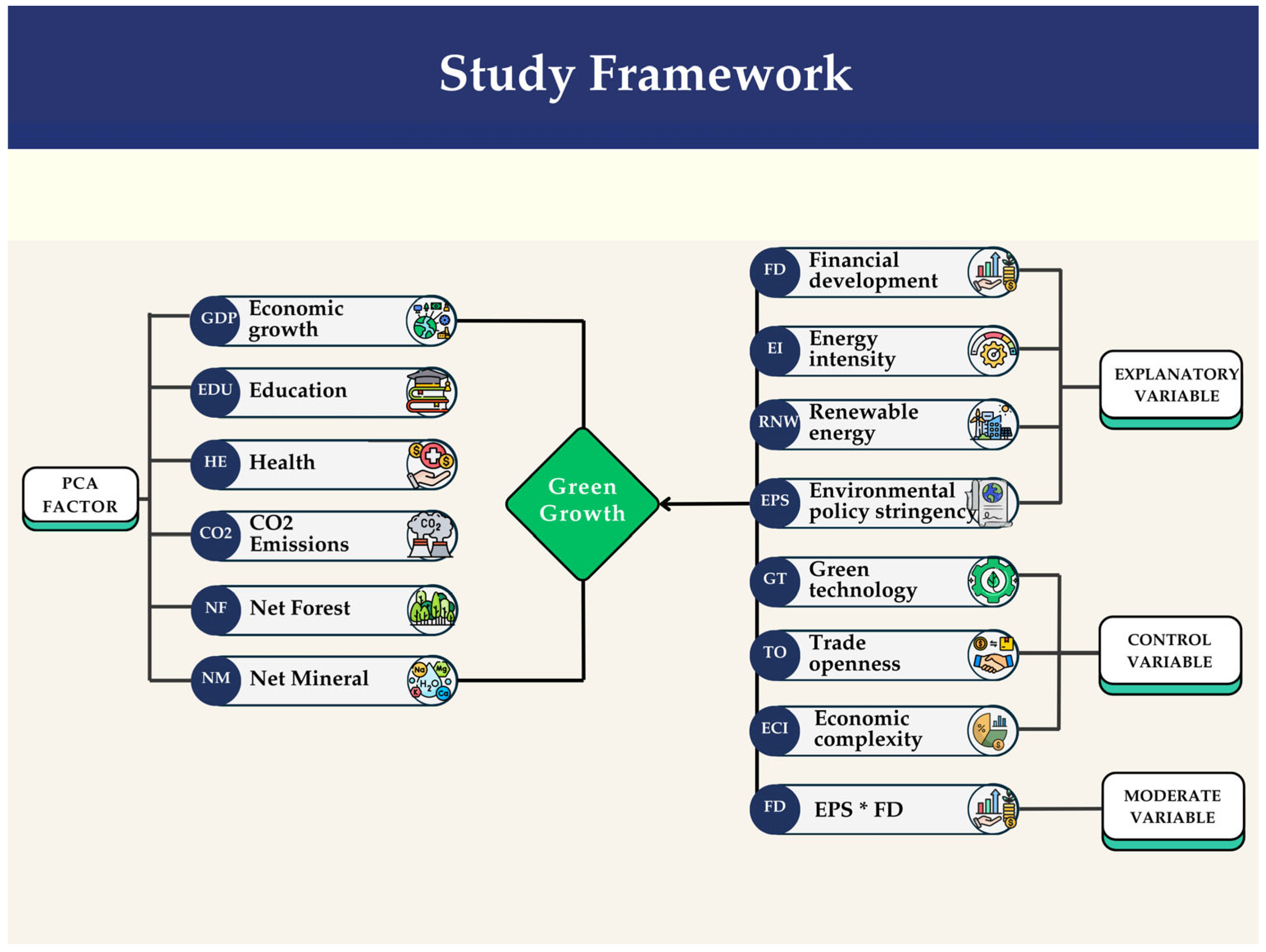
Variable	Variable Symbol	Variable Definitions	Source
Green growth	GG	GG index calculated by PCA analysis based on the dimensions of economic growth, educational, health expenditures, CO2 emissions, net forest, and mineral depletions.	WB
Financial development	FD	Financial Development Index	IMF
Energy intensity	EI	Primary energy consumption per GDP	Our World
Renewable energy	RNW	Renewable energy consumption (% of total final energy consumption)	WB
Environmental policy	EPS	Environmental Policy Stringency Index	OECD
Trade openness	TO	Trade (% of GDP)	WB
Green technology	GT	Development of environment-related technologies Index	OECD
Economic complexity	ECI	Economic Complexity Index	OEC
Elemental Indicators of GG	Symbol	Basic Indicators	Source
Economic growth	GDP	Gross domestic product growth (% annual)	WB
Education	EDU	School enrollment, secondary (% gross)	WB
Health	HE	Current health expenditure (% of GDP)	WB
CO2 Emissions	CO2	Carbon dioxide (CO2) emissions excluding LULUCF per capita (t CO2e/capita)	WB
Net Forest	NF	Adjusted savings: net forest depletion (% of GNI)	WB
Net Mineral	NM	Adjusted savings: mineral depletion (% of GNI)	WB

).

Since data for the HE and NF variables—components of the GG index—have only been available since 2000, this year marks the beginning of the dataset. The latest data for NM, FD, and RNW extend to 2021, while EDU and EI are available through 2022. For other variables, data from 2023 could be retrieved from the relevant databases. Considering these limitations, the dataset was extended to 2023 using the mean imputation technique to maintain temporal relevance.

As for the cross-sectional coverage of the panel data, the absence of ECI data for Estonia and Luxembourg, along with incomplete EDU data for the USA, Australia, and Japan, limited the sample to 23 countries: Austria, Belgium, Canada, Czechia, Denmark, Finland, France, Germany, Greece, Hungary, Ireland, Italy, Korea, Netherlands, New Zealand, Norway, Poland, Portugal, Slovak Republic, Spain, Sweden, Switzerland, and the United Kingdom.

3.2. Model Construction

The current study focuses on the impact of FD, RNW, EI, and EPS on GG and investigates the effects of the interaction of EPS and FD on GG. Equations (1) and (2) show the two main functions tested in the study.

$${GG}_{it}=f_1\left({FD}_{it},{EI}_{it},{RNW}_{it},{EPS}_{it},{TO}_{it}{,GT}_{it},{ECI}_{it}\right),$$

(1)

$${GG}_{it}=f_2\left({FD}_{it},{EI}_{it},{RNW}_{it},{EPS}_{it},{TO}_{it,}{GT}_{it},{ECI}_{it},{EPS}_{it}\times {FD}_{it}\right)$$

(2)

Models A and B are estimated based on the empirical functions. Model A (Equation (3)) investigates the long-run connection between GG and explanatory variables, while Model B (Equation (4)) explores the relationships between GG, explanatory variables, and EPS*FD.

$$\begin{array}{ll}{GG}_{it}={\beta }_0+{\beta }_1& Ln\left({FD}_{it}\right)+{\beta }_{2}Ln\left({EI}_{it}\right)+{\beta }_{3}Ln\left({RNW}_{it}\right)+{\beta }_{4}Ln\left({EPS}_{it}\right)+{\beta }_{5}Ln\left({TO}_{it}\right)+{\beta }_{6}Ln\left({GT}_{it}\right)\\ & +{\beta }_{7}Ln\left({ECI}_{it}\right)+{\mu }_{it}\end{array}$$

(3)

$$\begin{array}{ll}{GG}_{it}={\beta }_0+{\beta }_1& Ln\left({FD}_{it}\right)+{\beta }_{2}Ln\left(EI\right)+{\beta }_{3}Ln\left({RNW}_{it}\right)+{\beta }_{4}Ln\left({EPS}_{it}\right)+{\beta }_{5}Ln\left({TO}_{it}\right)+{\beta }_{6}Ln\left({GT}_{it}\right)\\ & +{\beta }_{7}Ln\left({ECI}_{it}\right)+{\beta }_{8}Ln\left({EPS}_{it}\right)\ast Ln\left({FD}_{it}\right)+{\mu }_{it}\end{array}$$

(4)

The i term in the model represents the 23 countries analyzed, while the t term represents 2000–2023. In addition, β₀ represents the constant coefficient, β₁–β₈ represent the coefficients of estimation, and u_it represents the model error term. The proposed model assumes that FD is positively associated with GG in OECD countries (β₁ > 0). EI is expected to affect GG negatively, whereas RNW is expected to contribute positively (β₂ < 0 and β₃ > 0). EPS is also presumed to have a positive connection with GG (β₄ > 0). Additionally, the analysis focuses on the interaction between FD and EPS in explaining GG (Model B). This interaction is hypothesized to enhance GG (β₈ < 0). ECI, TO, and GT are included as control variables. The effects of ECI and TO on GG may be either negative or positive (β₅ < 0 or β₅ > 0; β₇ < 0 or β₇ > 0), while GT is assumed to influence GG (β₆ > 0).

3.3. Methodology

In analyzing the econometric functions constructed within the study, the panel data analysis method is used, which allows both cross-sectional and time effects to be analyzed together. In this context, applying some preliminary tests is essential for the reliability and consistency of the model estimation. Normal distribution, endogeneity, multicollinearity, cross-sectional dependence (CSD), slope heterogeneity, and cointegration analyses are applied for panel data estimation. First, the correlation values between the series were calculated as shown in Equation (5) using the Spearman correlation test, which is preferred in the absence of the normality assumption.

$$r_s=1-{\displaystyle \frac{6{\sum }_{i=1}^n{d}_i^2}{n(n^2-1)}}$$

(5)

The endogeneity and multicollinearity problems observed during the estimation of the models may cause inconsistency in the model estimation results. To avoid inconsistency in model estimation, the endogeneity problem is examined by the Sargan–Hansen and the Block exogenous Wald test. Third, the multicollinearity problem is reviewed by the variance inflation factor (VIF) and the tolerance test. VIF shows how far the parameter estimates and variances deviate from their valid values due to the multicollinearity problem. The calculation of VIF and tolerance coefficient is shown in Equation (6).

$$VIF={\displaystyle \frac{1}{1-R^2}}={\displaystyle \frac{1}{Tolerance}}$$

(6)

Once the model specification is verified, the panel data analysis tests the assumptions of possible CDS and slope heterogeneity across OECD countries.

3.3.1. Cross-Sectional Dependency

The interaction of countries’ trade and economic activities has increased in the developing and changing world economy in recent years. As a result of this interaction, the interdependence of nations has also started to increase. CSD may be due to different economic dynamics among high-income countries. Different trade partnership structures, economic growth models, economic policies, and responses to financial shocks are indicators of CSD. As a result of these factors, the interdependence of cross-sectional units, or the fact that a shock in one of the cross-sectional units affects the other cross-sectional units, requires the study of CSD [71]. Considering the panel data set of the study, the bias-corrected LM test for CSD is applied using Equation (7) [72].

$${LM}_{adj}=\sqrt{{\displaystyle \frac{2T}{N\left(N-1\right)}}}{\sum }_{i=1}^{N-1}{\sum }_{j=i+1}^{N}T{\widehat{P}}_{ij}{\displaystyle \frac{\left(T-k\right)\widehat{P}{i}^{2}j-u_{Tij}}{\sqrt{u^2}{T}_{ij}}}$$

(7)

In Equation (7), $u_{Tij}$ is the mean while $\sqrt{u^2}{T}_{ij}$ is the variance. This test gives more significant results when T > N.

3.3.2. Slope Heterogeneity

The panel data set in the present study consists of OECD countries. Given the heterogeneity among these countries regarding economic, financial, and environmental policies, it is imperative to ascertain whether each variable series determined for this specific group of countries possesses a homogeneous or heterogeneous structure. Furthermore, it is necessary to determine the slope heterogeneity of the model error term to investigate the long-term cointegration connection between GG and the explanatory variables. To this end, the slope heterogeneity of the slope coefficients in the cointegration equation is analyzed using the Delta test proposed by Swamy [73] and developed by Pesaran and Yamagata [74]. The Delta test statistics are calculated using Equation (8) below [74].

$${\tilde{\mathsf{\Delta }}}_{\mathrm{a}\mathrm{d}\mathrm{j}}=\sqrt{\mathrm{N}}{\displaystyle \frac{{\mathrm{N}}^{-1 }\widehat{\mathrm{S}}-\mathrm{E}(\check{{\mathrm{Z}}_{\mathrm{i}\mathrm{t}})}}{\sqrt{\mathrm{V}\mathrm{a}\mathrm{r}}(\check{{\mathrm{Z}}_{\mathrm{i}\mathrm{t}})}}}~\mathrm{N}(0,1)$$

(8)

3.3.3. Unit Root Tests

The series stationarity should be examined to investigate the long-term cointegration connection between the variables and ensure the estimation results are robust, consistent, and reliable. The current study does not detect CSD for the series and models. In line with slope heterogeneity or homogeneity, first-generation unit root tests that do not consider CSD are preferred for the presence of a unit root in the series. In this context, the Levin et al. [75] (LLC) unit root tests are applied to slope homogeneous series, and the Im et al. [76] (IPS) unit root tests are applied to slope heterogeneous series. The LLC test allows different unit root tests for each cross-sectional unit [77]. This test is based on the t-statistic calculated as in Equation (9).

$$t_p={\displaystyle \frac{\widehat{p}}{SE\left(\widehat{p}\right)}}$$

(9)

This equation assumes that the residual series has white noise. The $t_p$ statistic in the panel model shows the convergence of the standard normal distribution when $N$ $and T \to \infty \sqrt{{\displaystyle \raisebox{1ex}{$N$}\!\left/ \!\raisebox{-1ex}{$T$}\right.}}\to 0$. Under these conditions, the LLC test statistics are shown in Equation (10).

$$t_p={\displaystyle \frac{t_{p}N T S_N{\widehat{\sigma }}^{-2}\left(\widehat{p}\right){\mu }_m^{*}}{{\sigma }_m^{*}}}$$

(10)

In the above equation, ${\mu }_m^{*}$ and ${\sigma }_m^{*}$ denote the modified error term and the error terms’ standard deviation, respectively, generated by the Monte Carlo Simulation Levin et al. [75]. The IPS fundamental assumption allows the autoregressive coefficient to be heterogeneous across cross-sectional units [77]. The model created in the IPS is reported in Equation (11).

$${∆y}_{i,t}={\alpha }_i+{\beta }_{i}t+{\rho }_i{y}_{i,t-1}+{\sum }_{j=1}^k{\mathrm{\varnothing }}_k{∆y}_{i,t-j}+u_{i,t}$$

(11)

In the IPS test, the ADF test is applied separately for all cross-sections that comprise the model. The panel’s test statistics are formed by standardizing the average of the calculated test statistics. Standardized panel root test statistics are as in Equation (12).

$$t_{IPS}={\displaystyle \frac{\sqrt{N({\overline{t}}_{NT}-E\left[t_{\mathrm{İ}T}\left|{\rho }_i=0\right.\right]}}{\sqrt{Var\left[t_{\mathrm{İ}T}\left|{\rho }_i=0\right.\right]}}}$$

(12)

The $\overline{t}$ value in the equation indicates the ADF test statistic calculated separately for each cross-section.

3.3.4. Panel Cointegration Tests

Following the findings regarding stationarity, CSD, and slope heterogeneity, which necessitate examination to ascertain the long-run relationships between variables within the context of panel data analysis, the Johansen [78] and Kao [79] tests were employed to assess the long-run cointegration connection between GG and the explanatory variables in the present study. It is determined that all series are non-stationary at level, do not contain CSD, and have heterogeneity. In this context, these two tests, which do not take CSD into account and can provide reliable and robust results under heterogeneity, were applied. The Johansen cointegration test used to examine the existence of a long-run and stable coupling between the series is shown in Equations (13) and (14).

$$∆{\mathsf{{\rm Y}}}_t={\mathsf{\Pi }}_{t-1}+{\sum }_{i=!}^{p-1}{\mathsf{\Gamma }}_i∆{\mathsf{{\rm Y}}}_{t-1}+B{x}_t+{\mu }_t$$

(13)

$$\mathsf{\Pi }={\sum }_{i=1}^p{A}_i-I,{\mathsf{\Gamma }}_i=-{\sum }_{\mathrm{İ}=1}^P{A}_i$$

(14)

In the given equations, $\Pi$ indicates the adjusted imbalance matrix. The stacking coefficient, A, demonstrates the rate of change of the endogenous factor concerning the imbalance. The $\Gamma$ indicator illuminates the capture of short-term dynamic adjustment. Johansen proposes two distinct likelihood ratio tests for the significance of the reduced order of the matrix $\Pi$. The propositions, the trace, and the maximum eigenvector tests are demonstrated in Equations (15) and (16), respectively.

$$J_{trace}=-T{\sum }_{i=r+1}^n\ln (1-{\widehat{\lambda }}_i)$$

(15)

$$J_{max}=-T\ln (1-{\widehat{\lambda }}_{i+1})$$

(16)

In the equation, T is the number of samples and ${\widehat{\lambda }}_i$ is the largest canonical correlation. In the current research, the Kao Residual Cointegration test is applied to strengthen the cointegration connection. In the Kao test, the Schwarz criterion estimator is used when there is an individual constant, and the Newey-West estimator is used to find the long-run variance. Moreover, the Kao [79] test considers the heterogeneity among cointegration vectors and rejects the endogeneity of independent variables due to asymptotic equivalence. Kao Residual Cointegration Test is reported in Equations (17)–(19).

$$y_{it}={\alpha }_i+\beta {\chi }_{it}+e_{it}$$

(17)

$$y_{it}=y_{it-1}+u_{i,t}$$

(18)

$${\chi }_{it}={\chi }_{it-1}+{\epsilon }_{it}$$

(19)

$$t=1,\dots \dots ,T;i=1,\dots \dots ,N$$

In the equations, $y_{it}$ and ${\chi }_{it}$ indicate the assumption that the series is stationary at I(1) and no differential cointegration occurs. However, Kao [79] argues for the equation $z_{it}=\left\{{\mu }_i\right\}$ and uses DF and ADF unit root tests for the ${\epsilon }_{it}$ series to reveal the cointegration relationship between the series.

3.3.5. Fully Modified Ordinary Least Squares (FMOLS)

Once the long-run cointegration relationships between the variables are revealed, it is essential to estimate the elasticity coefficients of the explanatory variables that are thought to impact the GG to formulate policies. In this context, the FMOLS technique proposed by Pedroni [80] determines the long-run connections between GG and FD, EI, RNW, and EPS, and the effect of FD*EPS interaction and control variables on GG. This technique considers endogeneity and autocorrelation problems and can asymptotically eliminate sampling bias [81]. Moreover, this model provides greater flexibility for heterogeneity [80]. The absence of CSD and the heterogeneity of all variables except EPS and TO are the reasons for using the FMOLS estimator in this study. FMOLS coefficients can be calculated using Equation (20).

$${\widehat{\beta }}_{FMOLS}^{*}=N^{-1}{\sum }_{n=1}^N{\widehat{\beta }}_{FMOLS,n}^{*}$$

(20)

In the equation, ${\widehat{\beta }}_{FMOLS,n}^{*}$ denotes the elasticity coefficient estimates for all cross-sections. To provide the robustness of the estimation findings in the present study, Ramsey’s RESET test for model specification errors, the Breusch–Godfrey LM test for autocorrelation, and the Breusch–Pagan–Godfrey test for heteroscedasticity are employed in the estimation models. Figure 2 shows all the processes regarding the panel data methodology applied in the current study.

4. Empirical Results

Pre-Test Results

The results of the descriptive statistics for the variables employed in the study are reported in

Table 2. Descriptive statistics and plots.

Box Plots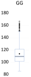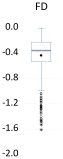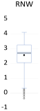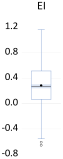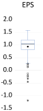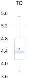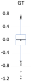
Stats.	GG	FD	RNW	EI	EPS	TO	GT	ECI
Mean	114.000	−0.435	2.572	0.284	0.938	4.488	0.002	0.115
Median	109.776	−0.362	2.721	0.272	1.051	4.396	0.014	0.281
Max.	167.260	−0.003	4.117	1.165	1.587	5.522	0.763	0.719
Min.	85.839	−1.611	−0.357	−0.657	−1.186	3.784	−1.178	−2.214
Std. Dev.	16.994	0.302	0.947	0.342	0.442	0.398	0.271	0.525
Skewness	1.153	−1.397	−0.810	0.037	−2.157	0.476	−0.254	−1.763
Kurtosis	3.802	4.870	3.553	2.930	9.214	2.179	4.341	6.104
J-B	137.1 ***	260.1 ***	67.340 ***	0.239 ***	1316.2 ***	36.306 ***	47.277 ***	507.6 ***
Obs.	552	552	552	552	552	552	552	552
Scatters plots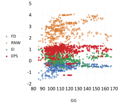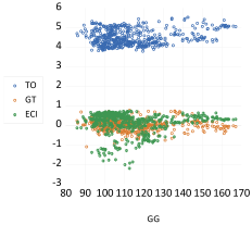

Note: *** p < 0.01.

. According to the findings, the mean value of FD is −0.435, RNW is 2.572, EI is 0.284, EPS is 0.938, TO is 4.488, GT is 0.002, and ECI is 0.115. While the dependent variable, GT, and the explanatory variables, EI and TO, have positive skewness values, the others exhibit negative skewness. However, the kurtosis values of all variables are positive. Jarque-Bera (J-B) values indicate normality and are statistically significant for all series. Based on these results, the null hypothesis of the J-B is rejected, confirming that the series does not follow a normal distribution. In addition, Table 2 presents a box plot, illustrating the maximum and minimum values and outliers. This table also includes scatter plots, facilitating a visual comparison of random distributions.

After examining the normality, the Spearman correlation was applied to calculate the correlations. The multicollinearity in the model is determined by calculating VIF and tolerance coefficients [82]. In

Table 3. Heat plot of correlation matrix.

1/VIF	VIF	GG	1.000	0.095	0.291	−0.223	0.169	0.094	−0.139	−0.132
0.599	1.669	FD	0.095	1.000	−0.071	−0.244	0.271	−0.322	−0.124	0.274
0.874	1.144	RNW	0.291	−0.071	1.000	−0.132	0.290	−0.093	0.169	−0.071
0.722	1.385	EI	−0.223	−0.244	−0.132	1.000	−0.375	−0.063	0.140	−0.137
0.600	1.668	EPS	0.169	0.271	0.290	−0.375	1.000	0.143	0.158	0.350
0.580	1.723	TO	0.094	−0.322	−0.093	−0.063	0.143	1.000	−0.130	0.262
0.783	1.276	GT	−0.139	−0.124	0.169	0.140	0.158	−0.130	1.000	−0.054
0.701	1.426	ECI	−0.132	0.274	−0.071	−0.137	0.350	0.262	−0.054	1.000
Mean VIF	(1.470)		GG	FD	RNW	EI	EPS	TO	GT	ECI

, VIF and tolerance coefficients are reported in addition to the correlation matrix results. A VIF coefficient of five and above and tolerance values of 0.2 and below [83] indicate a multicollinearity problem. Based on the VIF test results, the highest VIF among the explanatory variables was calculated for TO (1.723), and the lowest VIF was calculated for RNW (1.144). According to the tolerance coefficients, the variable with the highest tolerance value is RNW (0.874), and the variable with the lowest is TO (0.580). The correlation matrix has a positive connection between GG and FD, RNW, EPS, and TO, and a negative relationship between GG and EI, GT, and ECI. Moreover, the highest correlation between explanatory variables is between EI and EPS (−0.375), while the lowest is between GT and ECI (−0.054). According to VIF and tolerance values, the estimation model has no multicollinearity.

It is essential to examine multicollinearity and endogeneity when selecting valid variables for the accuracy of the model specification. Estimation without considering the endogeneity between the explanatory variables and the model’s error term may lead to unreliable results. The current study applies the Sargan–Hansen and Wald test (Block exogenous) for endogeneity (

Table 4. Endogeneity test results.

Block Exogenous Wald Test.
Hypothesis—H0: Exogenous		Chi-sq	Prob.
FD	RNW	1.843	0.606
	EI	0.992	0.803
	EPS	5.675	0.129
	TO	1.154	0.764
	GT	2.948	0.400
	ECI	5.959	0.114
RNW	FD	1.616	0.656
	EI	4.898	0.179
	EPS	6.075	0.108
	TO	3.405	0.333
	GT	5.619	0.132
	ECI	2.622	0.454
EI	FD	0.064	0.800
	RNW	0.001	0.970
	EPS	0.006	0.938
	TO	0.890	0.345
	GT	0.162	0.688
	ECI	0.026	0.871
EPS	FD	0.001	0.980
	RNW	0.005	0.946
	EI	3.508	0.061
	TO	3.031	0.082
	GT	0.100	0.752
	ECI	0.769	0.381
TO	FD	0.116	0.733
	RNW	0.140	0.709
	EI	0.052	0.820
	EPS	0.002	0.965
	GT	0.174	0.677
	ECI	0.650	0.420
GT	FD	1.039	0.308
	RNW	0.127	0.722
	EI	1.340	0.247
	EPS	0.387	0.534
	TO	0.241	0.624
	ECI	1.037	0.309
ECI	FD	1.608	0.205
	RNW	0.581	0.446
	EI	0.025	0.875
	EPS	0.021	0.885
	TO	0.658	0.417
	GT	0.001	0.974
Sargan–Hansen Test
Instrument specification:	Instrument	Sargan–Hansen J stat.	Prob(J-stat.)
@DYN(GG,-2) FD(-1) RNW(-1) EI(-1) EPS(-1) TO(-1) GT(-1) ECI(-1)	Model A	21.305	0.127
@DYN(GG,-2) FD(-1) RNW(-1) EI(-1) EPS(-1) TO(-1) GT(-1) ECI(-1) EPS*FD(-1)	Model B	18.972	0.165
H0: The instruments are valid

). As a result of the Wald test, statistically insignificant relationships between the explanatory variables are found, and these results indicate no endogeneity in the model. Sargan–Hansen test statistics and probabilities mean that the instrumental variables in the model are valid and do not contain endogeneity. Therefore, both tests confirm each other and are a strong indication that there is no endogeneity.

Another panel data analysis assumption is slope heterogeneity and CSD. In panel data analysis, ignoring slope heterogeneity and CSD leads to inconsistent estimation results.

Table 5. CSD and slope heterogeneity test results.

Variable	Bias-Cor. Scaled LM		Delta Tests
	Stat.	Prob.	$\tilde{\mathsf{\Delta }}$	Prob.	${\tilde{\mathsf{\Delta }}}_{\mathit{a}\mathit{d}\mathit{j}}$	Prob.
GG	−2.960	0.998	6.004	0.000	6.419	0.000
FD	−0.114	0.545	3.026	0.001	3.235	0.001
RNW	−4.125	1.000	2.568	0.005	2.746	0.003
EI	−1.251	0.894	4.406	0.000	4.710	0.000
EPS	−3.528	1.000	0.171	0.432	0.183	0.428
TO	0.835	0.202	0.669	0.252	0.715	0.237
GT	0.313	0.377	5.003	0.000	5.348	0.000
ECI	−4.878	1.000	1.818	0.034	1.944	0.026
Model A	1.015	0.155	5.078	0.000	6.348	0.000
Model B	−2.274	0.989	4.485	0.000	5.790	0.000

shows CSD and heterogeneity results on a variable and model basis. Since the study’s time and cross-sectional dimensions are close to each other, according to the Bias-corrected scaled LM results, the test’s null hypothesis cannot be rejected, proving there is no cross-sectional dependence on all series and models. However, according to the results of the delta test for slope heterogeneity, the EPS and TO series have slope homogeneity. In contrast, other variables and Models A and B have slope heterogeneity.

After determining CSD and slope heterogeneity, a stationarity analysis of the series should be performed. Unit root tests are essential for obtaining consistent findings in the study. Since CSD is not detected in this research, the unit root test is performed using the IPS developed by Im et al. [76] and the LLC created by Levin et al. [75], which are first-generation unit root tests. The unit root findings are shown in

Table 6. Unit root results.

	Intercept				Trend-Intercept
	IPS		LLC		IPS		LLC
	W Stat.	Prob.	t-Stat.	Prob.	W Stat.	Prob.	t-Stat.	Prob.
GG	1.997	0.977	0.261	0.603	−0.023	0.490	0.275	0.608
ΔGG	−11.578	0.000	−6.741	0.000	−9.023	0.000	−3.743	0.000
FD	−0.064	0.473	1.008	0.843	−1.398	0.081	−1.090	0.137
ΔFD	−12.592	0.000	−11.418	0.000	−11.081	0.000	−10.174	0.000
RNW	3.476	0.999	−1.147	0.125	−0.792	0.214	1.764	0.961
ΔRNW	−14.160	0.000	−15.149	0.000	−12.314	0.000	−12.385	0.000
EI	1.362	0.913	−1.018	0.154	0.172	0.568	0.246	0.597
ΔEI	−11.743	0.000	−4.960	0.000	−10.362	0.000	−4.406	0.000
EPS	−0.788	0.215	1.146	0.874	−0.642	0.260	2.010	0.977
ΔEPS	−6.591	0.000	−6.655	0.000	−6.486	0.000	−3.009	0.001
TO	2.037	0.979	−0.642	0.260	−0.616	0.268	0.901	0.816
ΔTO	−10.518	0.000	−4.335	0.000	−8.556	0.000	−3.284	0.000
GT	−0.371	0.355	−0.215	0.414	1.310	0.905	0.087	0.534
ΔGT	−17.427	0.000	−13.832	0.000	−10.580	0.000	−15.124	0.000
ECI	−1.206	0.113	0.185	0.573	−1.015	0.155	−0.146	0.441
ΔECI	−7.516	0.000	−3.115	0.000	−7.214	0.000	−2.020	0.021

. According to the unit root test results, all series include a unit root at the level but become stationary after the first difference. These findings allow us to investigate the cointegration linkage of the models tested in this study.

Examining the long-run cointegration connection between series in panel data analysis is possible after preliminary tests. In this study, Model A tests the long-run relationship between GG and FD, RWN, EI, and EPS, while Model B tests the interaction between GG and independent variables and EPS*FD. In the panel data of the current study, there is no slope heterogeneity and CSD. In this context, the tests of Johansen [78] and Kao [79] are applied to cointegration (

Table 7. Panel cointegration results.

Johansen Panel Cointegration
Model A	Hyp.		Trace	0.05
	No. of CE(s)	Eigenv.	Stat.	Crt. Val.	Prob
	None	0.493	1544.408	159.530	0.000
	No more than 1	0.478	1232.170	125.615	0.000
	No more than 2	0.402	933.310	95.754	0.000
	No more than 3	0.354	697.170	69.819	0.000
	No more than 4	0.305	496.243	47.856	0.000
	No more than 5	0.261	328.637	29.797	0.000
	No more than 6	0.219	189.452	15.495	0.000
	No more than 7	0.152	75.888	3.841	0.000
	Hyp.		Max-Eigen	0.05
	No. of CE(s)	Eigenv.	Stat.	Crt. Val.	Prob.
	None	0.493	312.238	52.363	0.000
	No more than 1	0.478	298.860	46.231	0.000
	No more than 2	0.402	236.139	40.078	0.000
	No more than 3	0.354	200.927	33.877	0.000
	No more than 4	0.305	167.606	27.584	0.000
	No more than 5	0.261	139.185	21.132	0.000
	No more than 6	0.219	113.565	14.265	0.000
	No more than 7	0.152	75.888	3.841	0.000
Model B	Hyp.		Trace	0.05
	No. of CE(s)	Eigenv.	Stat.	Crt. Val.	Prob.
	None	0.494	1745.055	197.371	0.000
	No more than 1	0.484	1431.569	159.530	0.000
	No more than 2	0.415	1127.091	125.615	0.000
	No more than 3	0.382	880.830	95.754	0.000
	No more than 4	0.345	659.440	69.819	0.000
	No more than 5	0.267	464.675	47.856	0.000
	No more than 6	0.245	321.539	29.797	0.000
	No more than 7	0.218	192.336	15.495	0.000
	No more than 8	0.158	79.307	3.841	0.000
	Hyp.		Max-Eigen	0.05
	No. of CE(s)	Eigenv.	Stat.	Crt. Val.	Prob.
	None	0.494	313.486	58.434	0.000
	No more than 1	0.484	304.478	52.363	0.000
	No more than 2	0.415	246.261	46.231	0.000
	No more than 3	0.382	221.391	40.078	0.000
	No more than 4	0.345	194.765	33.877	0.000
	No more than 5	0.267	143.136	27.584	0.000
	No more than 6	0.245	129.203	21.132	0.000
	No more than 7	0.218	113.029	14.265	0.000
	No more than 8	0.158	79.307	3.841	0.000
Kao Residual Cointegration
Model A	t-Statistic	Prob.	Model B	t-Statistic	Prob.
ADF	−10.641	0.000	ADF	−3.861	0.000
Residual var.	1.047556		Residual var.	1.047339
HAC var.	0.712478		HAC var.	0.712091

). Since cointegration between the variables is proven, Johansen’s cointegration results are estimated using the Panel Vector Error Correction Model (VECM). According to the Johansen test results, at most seven cointegration relationships for Model A and at most eight cointegration relationships for Model B. To support and reinforce these findings, the Kao cointegration test was used. As a result of this test, the H₀ hypothesis, which states no cointegration connection between the series, is rejected, and a cointegration relationship is revealed. These findings indicate that the explanatory variables of the research have a long-run connection in the green growth function for OECD countries over the period 2000–2023.

Following the preliminary tests applied before estimating the panel data models, the elasticity coefficients of the explanatory variables were calculated using the FMOLS method to reach the main findings (

Table 8. Estimation results.

	Model A				Model B
Variable	Coef.	Std. Er.	t-Stat.	Prob.	Coef.	Std. Er.	t-Stat.	Prob.
FD	−2.094	0.341	−6.135	0.000	−3.760	0.546	−6.885	0.000
EI	−1.861	0.141	−13.187	0.000	−1.669	0.153	−10.909	0.000
RNW	0.981	0.059	16.555	0.000	0.089	0.005	16.339	0.000
EPS	0.206	0.045	4.564	0.000	0.322	0.044	7.311	0.000
TO	−0.022	0.003	−7.223	0.000	−0.019	0.003	−5.575	0.000
GT	0.463	0.121	3.830	0.000	0.505	0.098	5.168	0.000
ECI	−0.333	0.120	−2.776	0.006	−0.238	0.118	−2.021	0.044
EPS*FD	-	-	-	-	0.444	0.195	2.280	0.023
	Stat.		Prob.		Stat.		Prob.
Ramsey’s Reset	0.882		0.378		0.627		0.530
Serial Correlation LM (Breusch–Godfrey)	1.699		0.115		1.168		0.132
Heteroskedasticity (Breusch–Pagan–Godfrey)	1.197		0.302		0.919		0.499
Adj. R2	0.716 ***				0.714 ***

*** denotes the significance of 5% level.

). Diagnostic tests for autocorrelation and heteroskedasticity confirm that the estimated results are reliable, robust, and consistent. Moreover, the Ramsey Reset test revealed that the explanatory variables do not have non-linear or higher-order effects on green growth. According to the findings from FMOLS estimations, financial development is negatively associated with green growth in OECD countries (β₁ < 0). Similarly, energy intensity reduces green growth (β₂ < 0). Conversely, our findings show that renewable energy consumption supports green growth (β₃ > 0). The study also focuses on the effect of stringent environmental policies on green growth. The findings show that stringent environmental policies increase green growth (β₄ > 0). Conversely, the study examines the influence of stringent environmental policies as a moderating factor in the connection between financial development and green growth (Model B). Accordingly, contrary to the direct negative effect of financial development on green growth, the interaction of financial development and stringent environmental policies increases green growth (β₈ > 0). Finally, the study includes trade openness, green technology, and economic complexity as control variables. Our findings show that economic complexity and trade openness reduce green growth (β₅ < 0, β₇ < 0), whereas green technology favors green growth (β₆ > 0).

Figure 3 provides a graphical summary of the estimation results. Our findings show that financial development, energy intensity, renewable energy, environmental policies, green technology, economic complexity, and trade openness play a determining role in green growth in OECD countries. Financial development does not directly support green growth in this group of countries. However, it should not be forgotten that financial development directly and indirectly affects other determinants. Improved financial systems can increase investments in renewable energy and green technology by facilitating the financing of green investments and increasing access to technologies that reduce energy intensity. Our findings support that the interaction of stringent environmental policies and financial development boosts green growth. Therefore, if environmental regulations are inadequate in these countries, the effect of financial development on green growth will be limited. Moreover, our findings suggest that economic complexity and trade openness negatively affect green growth. This may indicate that production may be concentrated in high-value-added but environmentally costly sectors. Similarly, trade openness may lead to the diffusion of more environmentally polluting products and modes of production. Therefore, to achieve green growth in OECD countries, policymakers must develop holistic policies compatible with each other and integrated with environmental objectives, considering all these possible factors.

5. Discussion

The impacts of financial development, energy intensity, and renewable energy on green growth in OECD countries are analyzed, and various findings are obtained. In addition, the moderating role of stringent environmental policies in the connection between financial development and green growth is examined, and comprehensive findings are obtained by considering green technology, economic complexity, and trade openness as control variables. According to our findings, financial development in OECD countries favors carbon-intensive sectors rather than moving towards renewable energy or sustainable technologies. In this context, Hypothesis 1 is accepted. This finding differs from the findings of Yang et al. [27] and Saqib et al. [3] but is in line with the findings of Ozkan et al. [9]. It is stated that financial development supports economic development but may also lead to environmental negativity [23]. Our findings support this view. This can be explained by channeling financial resources exclusively to economic growth, which may worsen environmental pollution by increasing energy consumption in fossil fuel-intensive industries. Financial development does not support green growth. Therefore, these countries should promote environmentally friendly financial instruments and green investments.

Our findings show that increasing energy intensity has a negative impact on green growth in OECD countries, whereas renewable energy consumption supports green growth. In this context, Hypothesis 2 and Hypothesis 3 are accepted. These findings are consistent with the results of Dzwigol et al. [56], Qamruzzaman and Karim [5], Saqib et al. [3], and Dzwigol et al. [42]. One of the key elements of sustainable economic development is energy intensity, which is determined by the amount of energy consumed to produce a unit of GDP. While low energy intensity can support environmental sustainability and promote economic growth, high energy intensity can cause environmental destruction and accelerate climate change [35]. Therefore, tightening energy efficiency regulations and promoting energy-efficient production models and technologies in this group of countries is essential. Energy efficiency and renewable energy are key strategies to tackle environmental challenges. Energy efficiency can reduce greenhouse gas emissions while supporting economic growth, and a transition to renewable energy can create a cleaner energy system to replace fossil fuels. The widespread use of renewable energy marks a significant transformation in the energy sector. It is argued that integrating renewable energy into production processes will reduce the negative impacts of carbon-intensive energy sources and support sustainable economic growth [47,48]. Our findings support these views. Hence, it is essential to prioritize energy efficiency policies and implement regulations that increase energy efficiency to support green growth in OECD countries.

Our findings further indicate that stringent environmental policies enhance green growth and serve as a moderating factor in the connection between financial development and green growth, by strengthening the effectiveness of financial systems in promoting environmentally sustainable outcomes. In this context, Hypothesis 4 is accepted. This finding is consistent with Chen and Tanchangya [63] and Feng et al. [64]. Strict environmental policies are essential for harmonizing environmental sustainability and economic development in OECD countries. Alalmaee [15] argues that strict environmental policies significantly affect financial markets in terms of both costs and opportunities. Strict regulations can limit profitability and investments by imposing additional financial burdens on businesses, but they can also contribute to the development of green finance by encouraging innovation. According to the ecological modernization approach, these policies can create a more resilient and sustainable economic structure. Our findings support this view. In this context, stringent environmental policies in OECD countries are essential for channeling financial resources towards renewable energy or sustainable technologies and ensuring green growth.

Our findings reveal that while green technology contributes positively to green growth, economic complexity, and trade openness are associated with reducing green growth. These findings are in line with those of Tawiah et al. [84], Lu et al. [13], and Dzwigol et al. [42]. There is a connection between levels of economic complexity and energy demand. Depending on their natural resources and import capacities, countries should build a balanced energy portfolio from different sources to provide the necessary energy while minimizing environmental impacts. A country’s production structure has a direct effect on the environment. As the economic structure becomes more complex, the need for more efficient processes in producing consumer goods increases, leading to increased environmental degradation [85]. Our findings support this view. However, existing studies on the environmental effects of trade openness reveal two contrasting findings. According to the Pollution Paradise Hypothesis, critics of internationalization argue that foreign investment and trade allow polluting activities to move from one country to another. On the other hand, it is also argued that trade openness can increase production efficiency by allowing a country to focus on sectors with a comparative advantage [84]. In this context, our findings show that increasing trade openness in OECD countries will negatively affect green growth and confirm the Pollution Paradise Hypothesis. Integrating environmental regulations into international trade policies in these countries is essential. Finally, green technologies offer opportunities for green growth in OECD countries. Therefore, it is crucial to adopt policies such as increasing financial support for green technologies and integrating them into industrial sectors.

However, OECD countries exhibit a heterogeneous structure, characterized by notable differences in financial development, technological capacity, environmental regulations, and energy policies. Therefore, the effects of our findings will not be realized at the same level for member states. For instance, while Scandinavian countries enforce robust environmental regulations, countries like Belgium, Canada, and the Czech Republic implement moderately stringent environmental policies. Similarly, significant variation exists in energy policy frameworks. Eastern European countries and South Korea rely heavily on coal, whereas Canada strongly depends on fossil fuel exports. In contrast, Norway demonstrates a high level of renewable energy consumption. Therefore, policy recommendations promoting green growth must consider these structural and implementation-related differences among countries to ensure their effectiveness and contextual relevance.

6. Conclusions and Policy Recommendations

This study focuses on the impact of financial development, renewable energy, energy intensity, and stringent environmental policies on green growth in OECD countries from 2000 to 2023. Additionally, the moderating role of stringent environmental policies in the connection between financial development and green growth is examined. Economic complexity, trade openness, and green technology are included as control variables to ensure a more comprehensive analysis. To identify these relationships, we first analyze the CSD between the variables using the Bias-corrected LM test. After evaluating the potential CSD effect, the stationarity level of the series is analyzed by panel unit root tests. Once the prerequisites are met, panel cointegration tests investigate the long-term connections between variables. Finally, the FMOLS method is applied to estimate the elasticity coefficients. The findings reveal that financial development and energy intensity reduce green growth, whereas strict environmental policies and renewable energy increase green growth. Moreover, the interaction of financial development and stringent environmental policies favors green growth. Finally, while the control variables, trade openness and economic complexity, negatively affect green growth, green technology increases green growth.

Based on the findings, some policy implications are drawn. (1) Financial development has a negative impact on green growth. For this reason, practices, and regulations that will harmonize the financial system with green growth should be implemented in OECD countries. Instead of directing financial resources only to industry-intensive sectors that increase environmental damage, environmentally friendly financial instruments and green investments should be supported in these countries. Incentives for renewable energy and green technologies can be provided by developing and promoting green financing instruments. On the other hand, it is also essential to implement policies by considering the differences in the financial systems of OECD countries. For example, France, Germany, and Sweden stand out in green finance practices. However, some member countries still face transition challenges and differences in regulation and enforcement. Conversely, our findings suggest that stringent environmental policies will reduce the negative effect of financial development on green growth in these countries. Adopting stringent environmental standards in these countries will therefore support green growth. (2) Energy intensity reduces green growth in OECD countries while increasing renewable energy consumption. Moreover, economic complexity negatively affects green growth. Economic complexity is associated with energy demand. Therefore, it is necessary to implement energy efficiency policies and provide incentives for renewable energy in these countries. It is recommended that energy-saving production processes be supported and regulations on energy use in industry be introduced. OECD countries also differ in terms of energy policies. The European region implements strict regulations on green transformation, but high coal dependency in Eastern Europe slows down green transformation processes. Korea is still highly dependent on coal, while Canada is dependent on energy-intensive industries and fossil fuel exports. OECD countries, therefore, face different challenges in their energy policies. These countries need to implement energy efficiency policies that consider their differences. (3) In these countries, environmental regulations in international trade policies stand out as a critical element. Moreover, it has been found that green technologies offer significant opportunities for green growth in OECD countries. In this context, it is necessary to implement policies that support the diffusion of green technologies in industrial sectors and increase financial incentives.

This research has several limitations. First, it focuses exclusively on high-income OECD countries from 2000 to 2023. Future analyses may enrich the findings by extending the time frame or incorporating a more diverse country sample. Additionally, although an overall evaluation of OECD countries is presented, significant differences exist among member states regarding economic, environmental, and technological development. Policy implications can be deepened through country- or region-specific studies to address this. Lastly, the analysis includes financial development, energy intensity, renewable energy, and stringent environmental policies as explanatory variables. Expanding the model to incorporate a broader set of economic, social, and environmental indicators may provide a more comprehensive understanding of the determinants of green growth.

References

- Kim, S.E.; Kim, H.; Chae, Y. A new approach to measuring green growth: Application to the OECD and Korea. Futures 2014, 63, 37–48. [Google Scholar] [CrossRef]
- OECD. Towards Green Growth; OECD: Paris, France, 2011; Available online: https://www.oecd.org/en/publications/towards-green-growth_9789264111318-en.html (accessed on 10 March 2025).
- Saqib, N.; Usman, M.; Ozturk, I.; Sharif, A. Harnessing the synergistic impacts of environmental innovations, financial development, green growth, and ecological footprint through the lens of SDGs policies for countries exhibiting high ecological footprints. Energy Policy 2024, 184, 113863. [Google Scholar] [CrossRef]
- Hickel, J.; Kallis, G. Is green growth possible? New Polit. Econ. 2020, 25, 469–486. [Google Scholar] [CrossRef]
- Qamruzzaman, M.; Karim, S. Green energy, green innovation, and political stability led to green growth in OECD nations. Energy Strategy Rev. 2024, 55, 101519. [Google Scholar] [CrossRef]
- Ngo, T.; Trinh, H.H.; Haouas, I.; Ullah, S. Examining the bidirectional nexus between financial development and green growth: International evidence through the roles of human capital and education expenditure. Resour. Policy 2022, 79, 102964. [Google Scholar] [CrossRef]
- Huang, J. Resources, innovation, globalization, and green growth: The BRICS financial development strategy. Geosci. Front. 2024, 15, 101741. [Google Scholar] [CrossRef]
- Anwar, A.; Huong, N.T.T.; Sharif, A.; Kilinc-Ata, N.; Çitil, M.; Demirtaş, F. Is a green world real or a dream? A look at green growth from green innovation and financial development: Evidence from fragile economies. Geol. J. 2024, 59, 98–112. [Google Scholar] [CrossRef]
- Ozkan, O.; Popescu, I.A.; Destek, M.A.; Balsalobre-Lorente, D. Time-quantile impact of foreign direct investment, financial development, and financial globalisation on green growth in BRICS economies. J. Environ. Manag. 2024, 371, 123145. [Google Scholar] [CrossRef]
- Shang, Y.; Lian, Y.; Chen, H.; Qian, F. The impacts of energy resource and tourism on green growth: Evidence from Asian economies. Resour. Policy 2023, 81, 103359. [Google Scholar] [CrossRef]
- Hao, L.N.; Umar, M.; Khan, Z.; Ali, W. Green growth and low carbon emission in G7 countries: How critical the network of environmental taxes, renewable energy, and human capital is? Sci. Total Environ. 2021, 752, 141853. [Google Scholar] [CrossRef]
- Razzaq, A.; Sharif, A.; Ozturk, I.; Skare, M. Asymmetric influence of digital finance, and renewable energy technology innovation on green growth in China. Renew. Energy 2023, 202, 310–319. [Google Scholar] [CrossRef]
- Lu, L.; Chen, Q.; Huang, R.; Usman, A. Education and its impact on renewable energy demand, carbon intensity, and green growth: Do digital financial inclusion and environmental policy stringency matter in China. Environ. Sci. Pollut. Res. 2023, 30, 12020–12028. [Google Scholar] [CrossRef] [PubMed]
- Xie, P.; Xu, Y.; Tan, X.; Tan, Q. How does environmental policy stringency influence green innovation for environmental managements? J. Environ. Manag. 2023, 338, 117766. [Google Scholar] [CrossRef]
- Alalmaee, H. Sustainability through policy stringency: Analysing the impact on financial development. Sustainability 2025, 17, 1374. [Google Scholar] [CrossRef]
- Ketchoua, G.S.; Arogundade, S.; Mduduzi, B. Revaluating the Sustainable Development Thesis: Exploring the moderating influence of technological innovation on the impact of foreign direct investment (FDI) on green growth in the OECD countries. Discov. Sustain. 2024, 5, 252. [Google Scholar] [CrossRef]
- OECD. Trust in Global Cooperation—The Vision for the OECD for the Next Decade; OECD: Paris, France, 2021; Available online: https://www.oecd.org/en/about/legal/trust-in-global-cooperation-the-vision-for-the-oecd-for-the-next-decade.html (accessed on 10 March 2025).
- Ahmed, F.; Kousar, S.; Pervaiz, A.; Shabbir, A. Do institutional quality and financial development affect sustainable economic growth? Evidence from South Asian countries. Borsa Istanb. Rev. 2022, 22, 189–196. [Google Scholar] [CrossRef]
- OECD. Finance and Investment for Environmental Goals; OECD: Paris, France, 2024; Available online: https://www.oecd.org/en/topics/finance-and-investment-for-environmental-goals.html (accessed on 10 March 2025).
- Singh, S.; Arya, V.; Yadav, M.P.; Power, G.J. Does financial development improve economic growth? The role of asymmetrical relationships. Glob. Financ. J. 2023, 56, 100831. [Google Scholar] [CrossRef]
- Elfaki, K.E.; Ahmed, E.M. Globalization and financial development contributions toward economic growth in Sudan. Res. Glob. 2024, 9, 100246. [Google Scholar] [CrossRef]
- Oroud, Y.; Almahadin, H.A.; Alkhazaleh, M.; Shneikat, B. Evidence from an emerging market economy on the dynamic connection between financial development and economic growth. Res. Glob. 2023, 6, 100124. [Google Scholar] [CrossRef]
- Yang, L.; Ni, M. Is financial development beneficial to improve the efficiency of green development? Evidence from the “Belt and Road” countries. Energy Econ. 2022, 105, 105734. [Google Scholar] [CrossRef]
- Danish; Baloch, M.A.; Mahmood, N.; Zhang, J.W. Effect of natural resources, renewable energy and economic development on CO2 emissions in BRICS countries. Sci. Total Environ. 2019, 678, 632–638. [Google Scholar] [CrossRef] [PubMed]
- Al-Mulali, U.; Tang, C.F.; Ozturk, I. Does financial development reduce environmental degradation? Evidence from a panel study of 129 countries. Environ. Sci. Pollut. Res. 2015, 22, 14891–14900. [Google Scholar] [CrossRef]
- Yin, Q. Nexus among financial development and equity market on green economic finance: Fresh insights from European Union. Renew. Energy 2023, 216, 118938. [Google Scholar] [CrossRef]
- Yang, C.; Qi, H.; Jia, L.; Wang, Y.; Huang, D. Impact of digital technologies and financial development on green growth: Role of mineral resources, institutional quality, and human development in South Asia. Resour. Policy 2024, 90, 104699. [Google Scholar] [CrossRef]
- Saint Akadiri, S.; Bekun, F.V.; Sarkodie, S.A. Contemporaneous interaction between energy consumption, economic growth and environmental sustainability in South Africa: What drives what? Sci. Total Environ. 2019, 686, 468–475. [Google Scholar] [CrossRef]
- Brożyna, J. Energy consumption and greenhouse gas emissions against the background of Polish economic growth. In Energy Transformation Towards Sustainability; Tvaronavičienė, M., Ślusarczyk, B., Eds.; Elsevier: Amsterdam, The Netherlands, 2020; pp. 52–70. [Google Scholar] [CrossRef]
- Xing, Y. Under the Goal of Sustainable Development, Do Regions with Higher Energy Intensity Generate More Green Innovation? Evidence from Chinese Cities. Sustainability 2024, 16, 6679. [Google Scholar] [CrossRef]
- Khan, M.K.; Babar, S.F.; Oryani, B.; Dagar, V.; Rehman, A.; Zakari, A.; Khan, M.O. Role of financial development, environmental-related technologies, research and development, energy intensity, natural resource depletion, and temperature in sustainable environment in Canada. Environ. Sci. Pollut. Res. 2022, 29, 622–638. [Google Scholar] [CrossRef]
- Ullah, O.; Zeb, A.; Shuhai, N.; Din, N.U. Exploring the role of green investment, energy intensity and economic complexity in balancing the relationship between growth and environmental degradation. Clean Technol. Environ. Policy 2024, 1–18. [Google Scholar] [CrossRef]
- Danish, M.; Ulucak, R.; Khan, S.U.D. Relationship between energy intensity and CO2 emissions: Does economic policy matter? Sustain. Dev. 2020, 28, 1457–1464. [Google Scholar] [CrossRef]
- Fiorito, G. Can we use the energy intensity indicator to study “decoupling” in modern economies? J. Clean. Prod. 2013, 47, 465–473. [Google Scholar] [CrossRef]
- Huang, W.; He, J. Impact of energy intensity, green economy, and natural resources development to achieve sustainable economic growth in Asian countries. Resour. Policy 2023, 84, 103726. [Google Scholar] [CrossRef]
- Díaz, A.; Marrero, G.A.; Puch, L.A.; Rodríguez, J. Economic growth, energy intensity and the energy mix. Energy Econ. 2019, 81, 1056–1077. [Google Scholar] [CrossRef]
- Mahmood, T.; Ahmad, E. The relationship of energy intensity with economic growth: Evidence for European economies. Energy Strat. Rev. 2018, 20, 90–98. [Google Scholar] [CrossRef]
- Suparjo, S.; Darma, S.; Kurniadin, N.; Kasuma, J.; Priyagus, P.; Darma, D.C.; Haryadi, H. Indonesia’s new SDGs agenda for green growth: Emphasis in the energy sector. Int. J. Energy Econ. Policy 2021, 11, 395–402. [Google Scholar] [CrossRef]
- Ernawati, E.; Syarif, M.; Suriadi, L.O.; Rosnawintang, R.; Madi, R.A. Does energy intensity correlate with economic growth and government governance? IOP Conf. Ser. Earth Environ. Sci. 2024, 1324, 012098. [Google Scholar] [CrossRef]
- Sarwar, S. Impact of energy intensity, green economy and blue economy to achieve sustainable economic growth in GCC countries: Does Saudi Vision 2030 matter to GCC countries. Renew. Energy 2022, 191, 30–46. [Google Scholar] [CrossRef]
- Pyra, M. The role of the green economy in shaping economic growth in Poland. Ann. Polish Assoc. Agric. Agrobuss. Econ. 2024, 26, 129–142. [Google Scholar] [CrossRef]
- Dzwigol, H.; Kwilinski, A.; Lyulyov, O.; Pimonenko, T. Digitalization and energy in attaining sustainable development: Impact on energy consumption, energy structure, and energy intensity. Energies 2024, 17, 1213. [Google Scholar] [CrossRef]
- Degirmenci, T.; Sofuoglu, E.; Aydin, M.; Adebayo, T.S. The role of energy intensity, green energy transition, and environmental policy stringency on environmental sustainability in G7 countries. Clean Technol. Environ. Policy 2024, 1–13. [Google Scholar] [CrossRef]
- Ackah, I.; Kizys, R. Green growth in oil-producing African countries: A panel data analysis of renewable energy demand. Renew. Sustain. Energy Rev. 2015, 50, 1157–1166. [Google Scholar] [CrossRef]
- Khan, A.; Khan, T.; Ahmad, M. The role of technological innovation in sustainable growth: Exploring the economic impact of green innovation and renewable energy. Environ. Chall. 2025, 18, 101109. [Google Scholar] [CrossRef]
- Behera, P.; Behera, B.; Sethi, N.; Handoyo, R.D. What drives environmental sustainability? The role of renewable energy, green innovation, and political stability in OECD economies. Int. J. Sustain. Dev. World Ecol. 2024, 31, 761–775. [Google Scholar] [CrossRef]
- Dai, H.; Xie, X.; Xie, Y.; Liu, J.; Masui, T. Green growth: The economic impacts of large-scale renewable energy development in China. Appl. Energy 2016, 162, 435–449. [Google Scholar] [CrossRef]
- Sohag, K.; Husain, S.; Hammoudeh, S.; Omar, N. Innovation, militarization, and renewable energy and green growth in OECD countries. Environ. Sci. Pollut. Res. 2021, 28, 36004–36017. [Google Scholar] [CrossRef]
- Li, R.; Wang, X.; Wang, Q. Does renewable energy reduce ecological footprint at the expense of economic growth? An empirical analysis of 120 countries. J. Clean. Prod. 2022, 346, 131207. [Google Scholar] [CrossRef]
- Saqib, N.; Ozturk, I.; Usman, M. Investigating the implications of technological innovations, financial inclusion, and renewable energy in diminishing ecological footprints levels in emerging economies. Geosci. Front. 2023, 14, 101667. [Google Scholar] [CrossRef]
- Joof, F.; Samour, A.; Ali, M.; Rehman, M.A.; Tursoy, T. Economic complexity, renewable energy, and ecological footprint: The role of the housing market in the USA. Energy Build. 2024, 311, 114131. [Google Scholar] [CrossRef]
- Wang, L.; Ye, F.; Lin, J.; Bibi, N. Exploring the impact of climate technology, financial inclusion and renewable energy on ecological footprint: Evidence from top polluted economies. PLoS ONE 2024, 19, e0302034. [Google Scholar] [CrossRef]
- Rahadian, D.; Anggadwita, G.; Firli, A.; Adibroto, A. Environmental impact of renewable energy projects: Life cycle assessment and ecological footprint. In Renewable Energy Projects and Investments Interdisciplinary Knowledge, Analysis, Opportunities, and Outlook; Dinçer, H., Yüksel, S., Eds.; Elsevier: London, UK, 2025; pp. 95–116. [Google Scholar]
- Danish, M.; Ulucak, R. How do environmental technologies affect green growth? Evidence from BRICS economies. Sci. Total Environ. 2020, 712, 136504. [Google Scholar] [CrossRef]
- Mohsin, M.; Taghizadeh-Hesary, F.; Iqbal, N.; Saydaliev, H.B. The role of technological progress and renewable energy deployment in green economic growth. Renew. Energy 2022, 190, 777–787. [Google Scholar] [CrossRef]
- Dzwigol, H.; Kwilinski, A.; Lyulyov, O.; Pimonenko, T. The role of environmental regulations, renewable energy, and energy efficiency in finding the path to green economic growth. Energies 2023, 16, 3090. [Google Scholar] [CrossRef]
- Murshed, M. Can renewable energy transition drive green growth? The role of good governance in promoting carbon emission-adjusted economic growth in Next Eleven countries. Innov. Green Dev. 2024, 3, 100123. [Google Scholar] [CrossRef]
- Li, Y.; Xu, H.; Li, H.; Xu, Y. Digital economy, environmental regulations, and green economic development. Finance Res. Lett. 2025, 75, 106858. [Google Scholar] [CrossRef]
- Chen, L.; Kenjayeva, U.; Mu, G.; Iqbal, N.; Chin, F. Evaluating the influence of environmental regulations on green economic growth in China: A focus on renewable energy and energy efficiency guidelines. Energy Strategy Rev. 2024, 56, 101544. [Google Scholar] [CrossRef]
- Martínez-Zarzoso, I.; Bengochea-Morancho, A.; Morales-Lage, R. Does environmental policy stringency foster innovation and productivity in OECD countries? Energy Policy 2019, 134, 110982. [Google Scholar] [CrossRef]
- Porter, M.E.; Linde, C.V.D. Toward a new conception of the environment-competitiveness relationship. J. Econ. Perspect. 1995, 9, 97–118. [Google Scholar] [CrossRef]
- Ahmed, K. Environmental policy stringency, related technological change and emissions inventory in 20 OECD countries. J. Environ. Manag. 2020, 274, 111209. [Google Scholar] [CrossRef]
- Chen, L.; Tanchangya, P. Analyzing the role of environmental technologies and environmental policy stringency on green growth in China. Environ. Sci. Pollut. Res. 2022, 29, 55630–55638. [Google Scholar] [CrossRef]
- Feng, M.; Zou, D.; Hafeez, M. Mineral resource volatility and green growth: The role of technological development, environmental policy stringency, and trade openness. Resour. Policy 2024, 89, 104630. [Google Scholar] [CrossRef]
- Arjomandi, A.; Gholipour, H.F.; Tajaddini, R.; Harvie, C. Environmental expenditure, policy stringency and green economic growth: Evidence from OECD countries. Appl. Econ. 2023, 55, 869–884. [Google Scholar] [CrossRef]
- Gao, X.; Yu, J.; Pertheban, T.R.; Sukumaran, S. Do fintech readiness, digital trade, and mineral resources rents contribute to economic growth: Exploring the role of environmental policy stringency. Resour. Policy 2024, 93, 105051. [Google Scholar] [CrossRef]
- Wang, W.; Imran, M.; Ali, K.; Sattar, A. Green policies and financial development in G7 economies: An in-depth analysis of environmental regulations and green economic growth. Nat. Resour. Forum 2024. [Google Scholar] [CrossRef]
- Lin, S.; Zhou, Z.; Hu, X.; Chen, S.; Huang, J. How can urban economic complexity promote green economic growth in China? The perspective of green technology innovation and industrial structure upgrading. J. Clean. Prod. 2024, 450, 141807. [Google Scholar] [CrossRef]
- Saud, S.; Haseeb, A.; Zaidi, S.A.H.; Khan, I.; Li, H. Moving towards green growth? Harnessing natural resources and economic complexity for sustainable development through the lens of the N-shaped EKC framework for the European Union. Resour. Policy 2024, 91, 104804. [Google Scholar] [CrossRef]
- Yousaf, M.; Khalid, S.; Sheikh, S.M.; Subhani, J. From Policy to Progress: Evaluating Institutional Quality, Trade Openness, FDI, and Green Technologies’ Role in Green Economic Growth Using an ARDL Approach in Emerging Asian Economies. J. Asian Dev. Stud. 2024, 13, 1022–1039. [Google Scholar] [CrossRef]
- Sarafidis, V.; Yamagata, T.; Robertson, D. A test of cross section dependence for a linear dynamic panel model with regressors. J. Econom. 2009, 148, 149–161. [Google Scholar] [CrossRef]
- Baltagi, B.H.; Feng, Q.; Kao, C. A Lagrange Multiplier test for cross-sectional dependence in a fixed effects panel data model. J. Econom. 2012, 170, 164–177. [Google Scholar] [CrossRef]
- Swamy, P.A. Efficient inference in a random coefficient regression model. Econometrica 1970, 38, 311–323. [Google Scholar] [CrossRef]
- Pesaran, M.H.; Yamagata, T. Testing slope homogeneity in large panels. J. Econom. 2008, 142, 50–93. [Google Scholar] [CrossRef]
- Levin, A.; Lin, C.F.; Chu, C.S.J. Unit root tests in panel data: Asymptotic and finite-sample properties. J. Econom. 2002, 108, 1–24. [Google Scholar] [CrossRef]
- Im, K.; Pesaran, H.; Shin, Y. Testing for unit roots in heterogeneous panels. J. Econom. 2003, 115, 53–74. [Google Scholar] [CrossRef]
- Baltagi, B.H. Econometric Analysis of Panel Data; John Wiley & Sons Inc.: West Sussex, UK, 2005. [Google Scholar]
- Johansen, S. Likelihood-Based Inference in Cointegrated Vector Autoregressive Models; Oxford University Press: New York, NY, USA, 1995. [Google Scholar]
- Kao, C. Spurious regression and residual-based tests for cointegration in panel data. J. Econom. 1999, 90, 1–44. [Google Scholar] [CrossRef]
- Pedroni, P. Fully modified OLS for heterogeneous cointegrated panels. In Nonstationary Panels, Panel Cointegration, and Dynamic Panels; Baltagi, B.H., Fomby, T.B., Carter Hill, R., Eds.; Emerald Group Publishing Limited: Leeds, UK, 2001; pp. 93–130. [Google Scholar]
- Narayan, S.; Narayan, P.K. Determinants of demand for Fiji’s exports: An empirical investigation. The Developing Economies 2004, 42, 95–112. [Google Scholar] [CrossRef]
- Singh, S.G.; Kumar, S.V. Dealing with multicollinearity problem in analysis of side friction characteristics under urban heterogeneous traffic conditions. Arab. J. Sci. Eng. 2021, 46, 10739–10755. [Google Scholar] [CrossRef]
- Abbass, K.; Amin, N.; Khan, F.; Begum, H.; Song, H. Driving sustainability: The nexus of financial development, economic globalization, and renewable energy in fostering a greener future. Energy Environ. 2025, 1, 1–23. [Google Scholar] [CrossRef]
- Tawiah, V.; Zakari, A.; Adedoyin, F.F. Determinants of green growth in developed and developing countries. Environ. Sci. Pollut. Res. 2021, 28, 39227–39242. [Google Scholar] [CrossRef]
- Balsalobre-Lorente, D.; Nur, T.; Topaloglu, E.E.; Evcimen, C. Assessing the impact of the economic complexity on the ecological footprint in G7 countries: Fresh evidence under human development and energy innovation processes. Gondwana Res. 2024, 127, 226–245. [Google Scholar] [CrossRef]