Prediction of Transformer Residual Flux Based on J-A Hysteresis Theory

Abstract

Circuit breakers are effectively utilized for the controlled switching technique to mitigate inrush current when energizing an unloaded transformer. The core of the controlled switching technique is to obtain the appropriate closing angle based on the residual flux after opening. For the prediction of residual flux, the voltage integration method faces the difficult problem of determining the integration upper limit, while the Jiles- Atherton (J-A) model has the advantages of clear physical meaning of parameters, accurate calculation, and the ability to iteratively solve residual magnetism. It has low dependence on the initial conditions and greatly avoids the influence of DC offset and noise on measurement results. Firstly, an improved particle-swarm optimization algorithm is proposed in this paper to address the problem of slow convergence speed and susceptibility to local optima in current particle-swarm optimization algorithms for extracting J-A model parameters. The problem of slow convergence speed and susceptibility to local optima in traditional particle-swarm optimization algorithms is solved by optimizing the velocity and position-update formulas of particles in this algorithm. This new algorithm not only accelerates convergence speed, but also balances the overall and local search capabilities. Then, based on the J-A model, residual flux prediction of the transformer is carried out, and a transformer no-load energization experimental platform is built. A simulation model combining the J-A model and classical transformer is constructed using PSCAD/EMTDC to predict the residual flux of the transformer at different closing angles. Finally, by combining simulation with actual experimental waveform data, the accuracy of residual flux prediction was verified by comparing the peak values of the inrush current.

1. Introduction

During the random energization process of unloaded transformers, inrush currents that far exceed the rated current may be induced, which can cause damage to the safety and stability of the power system [1,2]. To address this issue, the controlled switching technique [3] is commonly used. That is, based on the value of the residual flux at the time of disconnection, closing is performed at the optimal phase to ensure a smooth transition of the flux. Thereby, the phenomenon of magnetizing inrush current is effectively suppressed as a result [4,5,6,7].

To determine the best closing phase, accurate residual flux values are required. Currently, the commonly used calculation methods are the voltage integration method and the hysteresis model method. The voltage integration method estimates the residual flux value by integrating the port voltage, but this method has the problem of low accuracy, and it is also difficult to determine the upper and lower limits of integration in practical applications. In addition, the presence of DC offset in the voltage signal can accumulate over time after integration, leading to significant deviations in the estimation of magnetic flux. In the hysteresis model method, the most widely used is the physically meaningful J-A model [8,9,10,11,12]. It is capable of iteratively solving for remanence, exhibits a lower dependency on initial conditions, and significantly mitigates the impact of DC offset and noise on measurement outcomes.

The identification results of the model parameters directly affect the prediction effect of the J-A model. Currently, many intelligent algorithms, such as genetic algorithms, frog-leap algorithms, PSO algorithms, etc., are widely used to extract J-A model parameters. However, these algorithms have some problems, such as slow convergence speed and a tendency to fall into local optimal solutions.

To solve these problems, an improved PSO algorithm with adaptively updated speed and position is proposed in this paper. The identification accuracy of the improved algorithm is significantly higher than that of traditional algorithms. In addition, a transformer model based on the J-A model is built using PSCAD/EMTDC to simulate the circuit breaker’s unloaded energization on the transformer, considering the influence of DC bias flux while providing a residual flux prediction model. After filtering out the influence of DC bias flux, the effectiveness of the residual flux prediction method is verified by comparing the peak values of inrush currents in simulation and experiment.

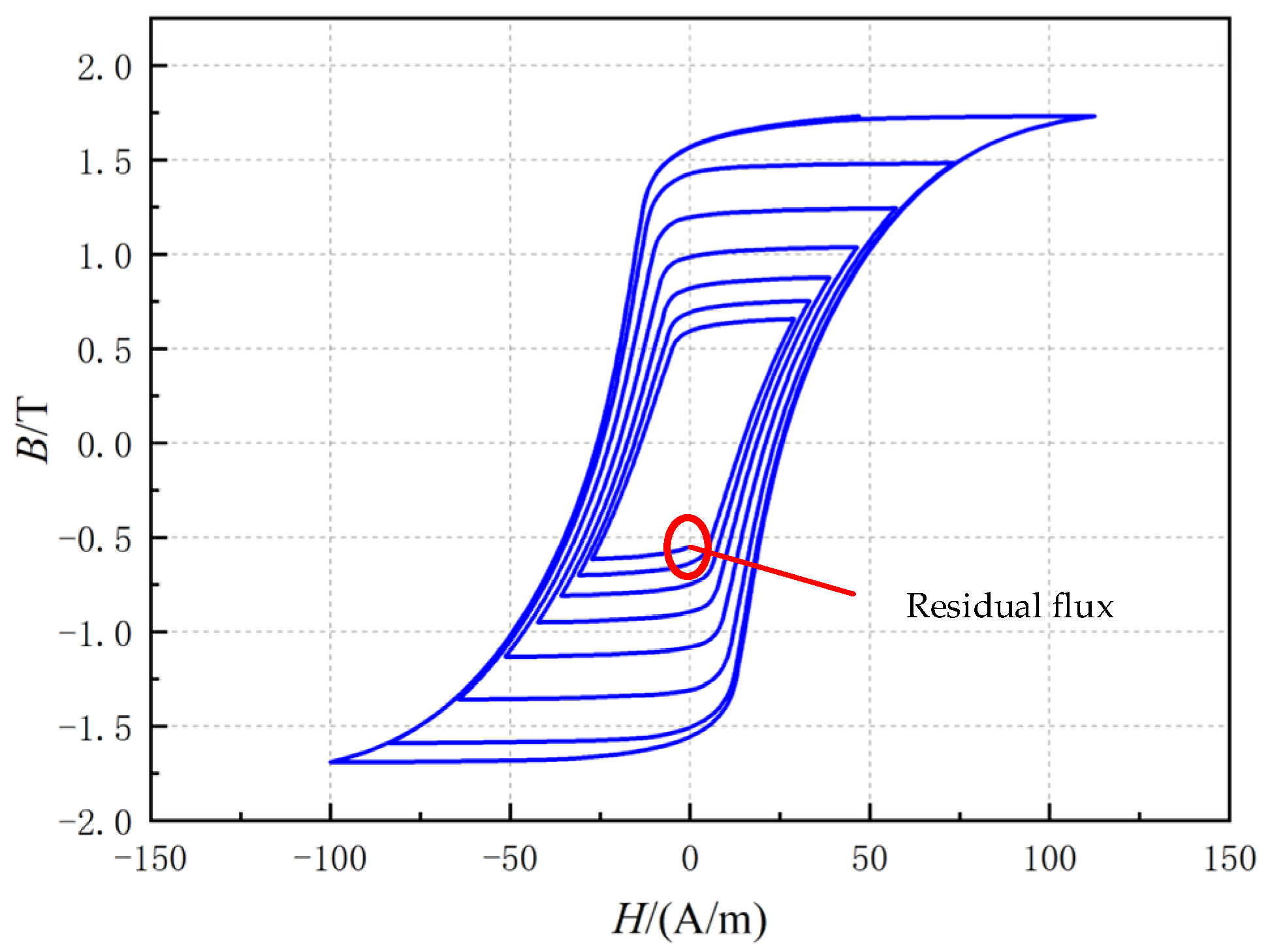
2. J-A Hysteresis Model

The J-A hysteresis model is a physical model based on the principles of domain-wall motion and energy conservation, which is founded on the theory of magnetic domains to describe the nonlinear hysteresis characteristics of ferromagnetic materials. In this hysteresis model, the actual magnetization intensity M is decomposed into reversible magnetization M_rev and irreversible magnetization M_irr, that is:

$$M=M_{irr}+M_{rev}$$

(1)

In Equation (1), the bending of the domain walls causes the reversible magnetization component, and the replacement of domain walls causes the irreversible magnetization component. The ordinary differential equation associated with the irreversible magnetization intensity M_irr is:

$${\displaystyle \frac{\mathrm{d}{M}_{irr}}{\mathrm{d}{H}_e}}={\displaystyle \frac{{\delta }_M\left(M_{an}-M_{ir}\right)}{k\delta }}$$

(2)

$$H_e=H+\alpha M$$

(3)

$$M_m=M\left\{\coth \left({\displaystyle \frac{H+\alpha M}{a}}\right)-\left[{\displaystyle \frac{a}{H+\alpha M}}\right]\right\}$$

(4)

$${\delta }_M=\left\{\begin{array}{ll}1\hfill & \mathrm{sgn}(M_{an}-M)\cdot \mathrm{sgn}(\mathrm{d}H/\mathrm{d}t)\ge 0\hfill \\ 0\hfill & \mathrm{sgn}(M_{an}-M)\cdot \mathrm{sgn}(\mathrm{d}H/\mathrm{d}t)<0\hfill \end{array}\right.$$

(5)

In the equation, H_e represents the effective magnetic field strength; M_an represents the anhysteretic magnetization, which is described by the Langevin function. In the equation, δ_M is a coefficient introduced to prevent non-physical solutions; δ is the direction coefficient, $\mathrm{d}H/\mathrm{d}t<0,\eta =-1$; $\mathrm{d}H/\mathrm{d}t>0,\eta =1$; and M_s, α, and a represent the saturation magnetization, the average field parameter of the internal coupling within the magnetic domain, and the shape parameter of the anhysteretic magnetization curve, respectively. The relationship between M_an, M_rev, and M_irr is:

$$M_{rev}=c\left(M_{an}-M_{ir}\right)$$

(6)

In the equation, c is the reversible magnetization coefficient. The energy conservation equation is:

$${\mu }_0{\delta }_M{\displaystyle \int M} \mathrm{d}{H}_e={\mu }_0{\delta }_M{\displaystyle \int M_{an}}\mathrm{d}{H}_e-{\mu }_{0}k\eta {\displaystyle \int \left(\frac{ \mathrm{d}{M}_{ir\eta }}{ \mathrm{d}{H}_e}\right)}\mathrm{d}{H}_e$$

(7)

In the equation, k is the pinning coefficient between magnetic domains. Based on the aforementioned equations, the J-A model obtained is:

$${\displaystyle \frac{\mathrm{d}M}{ \mathrm{d}H}}={\displaystyle \frac{{\delta }_M(1-c)\left(M_{an}-M\right)+k\eta c\cdot \frac{ \mathrm{d}{M}_{an}}{ \mathrm{d}H}}{k\eta -\alpha {\delta }_M(1-c)\left(M_{an}-M\right)}}$$

(8)

In the J-A model, each parameter exerts a more or less significant influence on the remanence value, and each parameter distinctly affects the hysteresis loop. The parameter M_s plays a pivotal role in the analysis of the hysteresis loop, primarily regulating the maximum magnetization on the loop and the susceptibility at the coercivity point. The parameters k and c collectively determine the magnitude of coercivity and the area enclosed by the loop, yet they exert opposing effects on the loop’s characteristics. The setting of parameter α directly impacts the susceptibility at the coercivity point. Parameter a influences the extent of the knee region in the hysteresis loop. To elucidate the impact of these parameters on the hysteresis loop more clearly, the effects of each parameter on the characteristic quantities of the hysteresis loop are summarized in

Table 1. The influence of parameters on hysteresis loop.

Parameters	Residual Flux	Coercivity	Coercivity Susceptibility	Hysteresis Loop Area	Maximum Magnetization
Ms increase	Increase	Remain	Increase	Remain	Increase
α increase	Increase	Remain	Increase	Remain	Remain
a increase	Decrease	Remain	Decrease	Remain	Remain
k increase	Increase	Increase	Remain	Increase	Remain
c increase	Decrease	Decrease	Remain	Decrease	Remain

.

3. Parameter Identification Method

Set the fitness function as the difference between the magnetic-field intensity curve calculated from the J-A model parameters and the target magnetic-field intensity curve.

To accurately assess the analytical precision of optimization algorithms, a highly sensitive error evaluation metric, the root mean square error (RMSE), is adopted as the objective function (or fitness value) for optimization [13,14]. By minimizing this objective function, the problem of J-A model parameter identification can be transformed into an optimization problem, thereby enhancing the accuracy of parameter identification. The objective function is:

$$Fitness=\sqrt{{\displaystyle \frac{{\displaystyle \sum _{i=1}^N{\left(H_{mea}(i)-H_{cal}(i)\right)}^2}}{N}}}$$

(9)

In the equation, H_mea represents the measured value of the magnetic field strength; H_cal represents the calculated value of the magnetic field strength; N represents the number of experimental sampling points and it is set to 20 in subsequent experiments.

3.1. Standard PSO Algorithm

Within the framework of the standard particle-swarm optimization (PSO) algorithm, each particle searches by referring to its own best position in the past (pbest) and the best position discovered by the entire swarm (gbest) in order to locate the optimal solution. For an optimization problem defined by the variable set X = {x₁, x₂,…, x_D} and aiming to minimize the function min{f(x)}, the position-update formula for a particle is:

$$v_{id}(t+1)=w{v}_{id}(t)+c_1{r}_1({\mathrm{pbest}}_{id}-x_{id}(t))+c_2{r}_2({\mathrm{gbest}}_d-x_{id}(t))$$

(10)

$$x_{id}(t+1)=x_{id}(t)+v_{id}(t+1)$$

(11)

At time step t + 1, the velocity and position of particle i are represented by v_id (t + 1) and x_id (t + 1), respectively, where w represents the inertia weight coefficient; c₁ and c₂ are the individual learning factor and the social learning factor, respectively; r₁ and r₂ are two random variables uniformly distributed in the interval [0, 1], used for the update of particle position and velocity. However, the algorithm control parameters (such as particle initialization, inertia weight, learning factors, etc.) determine the search capability of the algorithm, and these parameters also affect the balance between global exploration and local fine-tuning of the algorithm. This leads to deficiencies in the local search capability and search precision of the standard PSO algorithm [15,16].

3.2. Improved Algorithm

This paper proposes an improved adaptive velocity and position-update method, where the individual best and global best are replaced with linear combinations in Equation (10) for pbest_id and gbest_d, respectively. This leads to a new velocity update strategy, as shown in Equation (12).

$$v_{id}(t+1)=w_{id}(t)+c_1{r}_1\left({\displaystyle \frac{{ \mathrm{pbest} }_{id}+{ \mathrm{gbest} }_d}{2}}-x_{id}(t)\right)+c_2{r}_2\left({\displaystyle \frac{{ \mathrm{pbest} }_{id}-{ \mathrm{gbest} }_d}{2}}-x_{id}(t)\right)$$

(12)

The linear combination of pbest_id and gbest_d is equivalent to the original combination of two vectors, where the magnitudes of the two new vectors are amplified through linear combination. This allows the algorithm to expand the search area in the early stages, facilitating the identification of the region where the global optimal solution resides.

Furthermore, the average value of each particle’s information across all dimensions is calculated to adjust the particle’s position-update strategy, thereby enhancing the algorithm’s performance. Introduce the average of the information of each particle across all dimensions, as shown in Equation (13).

$$p_{ad}(t)={\displaystyle \frac{1}{D}}{\displaystyle \sum _{i=1}^D{x}_{id}}(t)$$

(13)

To balance the effects of local and global search throughout the iteration process, pad is used to replace pbest_id, eliminating the need to recalculate pbest_id in each iteration, thereby accelerating the convergence speed of the algorithm. Two different position-update strategies are employed: one is “X = X + V”, mainly used to enhance local search capabilities; the other is “X = wX + (1 − w)V”, primarily used to strengthen global search capabilities, as shown in Equations (14) and (15).

$$p_i={\displaystyle \frac{\exp \left(\mathrm{fit}\left(x_i(\mathrm{t})\right)\right)}{\exp \left({\displaystyle \frac{1}{N}}{\displaystyle \sum _{i=1}^N\mathrm{fit}}(x_i(t))\right)}}$$

(14)

$$x_{id}(t+1)=\left\{\begin{array}{ll}w{x}_{id}(t)+(1-w)v_{id}(t+1),\hfill & p_i> \mathrm{rand} \hfill \\ x_{id}(t)+v_{id}(t+1),\hfill & \mathrm{else} \hfill \end{array}\right.$$

(15)

In the equation, fit is used to measure the fitness of each particle, and N defines the total number of particles in the swarm. In Equation (14), the fitness ratio pi for each particle is used to measure the relative value between the individual particle’s fitness and the average fitness of the entire swarm. When a particle is in a relatively good position, its fitness value will be significantly higher than the average, and in this case, the update strategy “X = wX + (1 − w)V” is adopted to utilize the information from its current position for global search; conversely, if the particle’s fitness value is close to or below the average, it indicates a need for more intensive local search, and in this case, the strategy “X = X + V” is employed.

The new velocity and position-update formulas are as shown in Equations (16) and (17).

$$\left\{\begin{array}{l}{v}_{id}(t+1)=w{v}_{id}(t)+c_1{r}_1\left({\displaystyle \frac{{ \mathrm{pbest} }_{id}+{ \mathrm{gbest} }_d}{2}}-x_{id}(t)\right)\\ +c_2{r}_2\left({\displaystyle \frac{{ \mathrm{pbest} }_{id}-{ \mathrm{gbest} }_d}{2}}-x_{id}(t)\right)\\ x_{id}(t+1)=w{x}_{id}(t)+(1-w)v_{id}(t+1)\end{array}\right.$$

(16)

$$\left\{\begin{array}{l}{v}_{id}(t+1)=w{v}_{id}(t)+c_1{r}_1\left(p_{ad}-x_{id}(t)\right)+c_2{r}_2\left({ \mathrm{gbest} }_d-x_{id}(t)\right)\hfill \\ x_{id}(t+1)=x_{id}(t)+v_{id}(t+1)\hfill \end{array}\right.$$

(17)

An adaptive update strategy is employed to dynamically adjust the velocity and position of particles based on the comparison between the fitness ratio p_i and a predetermined threshold δ. When p_i > δ, that is, when the fitness of an individual particle is significantly higher than the average fitness of the population, this usually indicates that the algorithm is in the exploration phase or the particles are relatively dispersed. In this case, the update method of Equation (16) is used, which combines the linear combination of individual best positions and global best positions to expand the search range of particles. For position updates, the global search capability is strengthened by using “X = wX + (1 − w)V”. Conversely, when p_i < δ, it indicates that the fitness of an individual particle is close to the average fitness of the population, which means the algorithm is conducting an in-depth local search or the particles have tended to aggregate. At this stage, it is more appropriate to adopt the strategy of Equation (17), which enhances the algorithm’s local exploration capability and prevents premature convergence to local optima when solving complex multimodal problems. Additionally, introducing average dimensional information in the velocity-update process enables the algorithm to converge more quickly.

With this adaptive update mechanism, the algorithm can flexibly adjust the exploration strategy based on the search phase and the distribution of particles, effectively expanding the search range to find the global optimal solution, and at the same time, strengthening the local search when necessary, with the aim of achieving better search results and faster convergence speeds.

The steps of the improved PSO algorithm can be summarized in the following stages:

Initialization process: In this stage, the basic parameters of the algorithm are set, such as the population size N, the maximum number of iterations K, learning factors, inertia weights, etc. At the same time, initial positions and velocities are randomly assigned to each particle within the predetermined search space.

Fitness evaluation: Using the pre-set objective function, the fitness value of each particle in the population is calculated for use in the subsequent optimization process.

Updating global and personal best: Compare the current fitness of each particle with its past best fitness one by one. If the current fitness is better than the historical best fitness, update the particle’s position as the optimal position; otherwise, keep it unchanged.

Dynamic update of velocity and position: Calculate the fitness ratio p_i for each particle. If p_i is greater than the threshold δ, it indicates that a global search optimization is needed, and then the velocity and position of the particles are promptly adjusted according to the update strategy in Equation (16). Conversely, if p_i < δ, it suggests that the local search capability should be strengthened, and the velocity and position are updated using Equation (17).

Termination condition check: During the execution of the algorithm, check whether the stopping conditions are met, that is, whether the maximum number of iterations is reached or sufficient optimization is achieved. If the conditions are met, the algorithm will stop and output the final results; if not, the algorithm will return to step two to continue iterating.

Through the aforementioned steps, the improved algorithm can flexibly adjust between global and local searches, effectively finding the optimal solution to the problem.

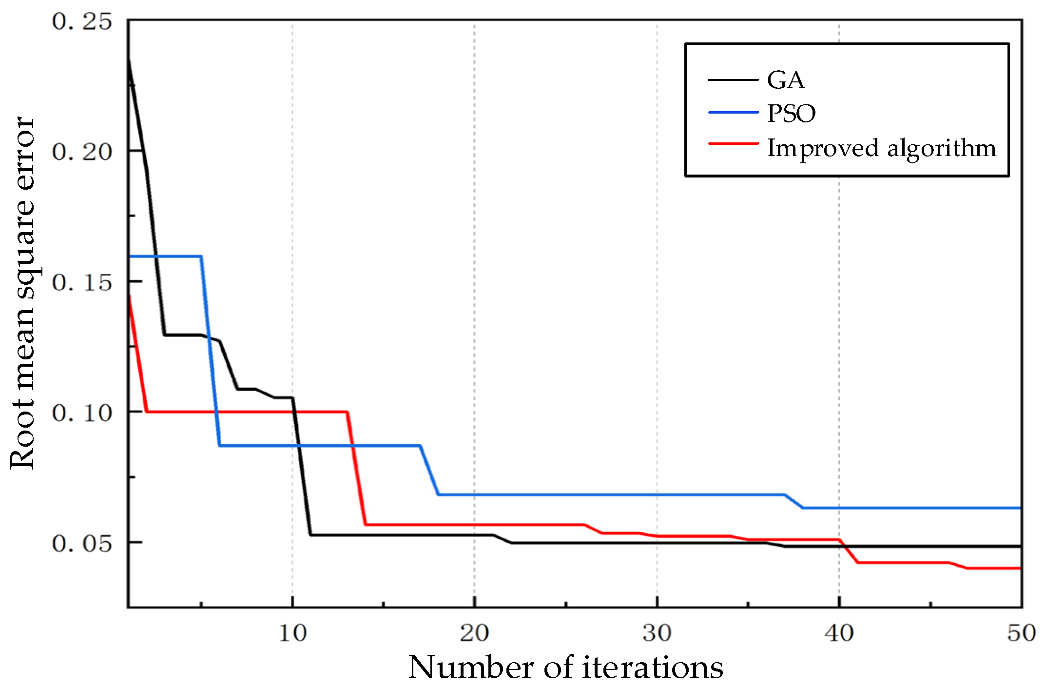
4. Algorithm Feasibility Validation

To validate the feasibility and effectiveness of the improved algorithm proposed in this paper for parameter identification in the J-A model, a set of hysteresis loops generated by custom parameters were used as theoretical curves. In the experiment, in addition to applying the improved PSO and traditional PSO algorithms, the genetic algorithm (GA) was also utilized to identify the static hysteresis parameters of the JA model [17]. The results, as shown in Figure 1, clearly demonstrate that the fitting effect of the improved algorithm is superior to that of the traditional algorithm. Furthermore, it is evident from

Table 2. Comparison of parameter identification results.

Algorithm	k	α	a	Ms	c
Theoretical Value	50	8 × 10−5	30	1.53 × 106	0.7
GA	69.6979	5.208 × 10−5	13.992	1.485 × 106	0.561
PSO	66.593	1 × 10−4	46.767	1.586 × 106	0.513
Improved Algorithm	54.765	9.422 × 10−5	35.473	1.576 × 106	0.622

that the improved algorithm significantly outperforms the traditional PSO algorithm and the GA in terms of parameter identification accuracy. The maximum relative error of the traditional algorithm is 55.9%, while the maximum relative error of the improved algorithm is reduced to 17.6%.

Additionally, to characterize the convergence speed of the aforementioned algorithms, Figure 2 presents the trend of the root mean square error of each algorithm as a function of the number of iterations.

The traditional algorithm exhibits a pronounced premature convergence phenomenon, getting stuck in a local optimum by the 11th iteration, and its global search capability is poor. The improved algorithm can escape from local optima multiple times because it adopts different velocity and position-update strategies according to different situations to re-determine the region of the global optimum.

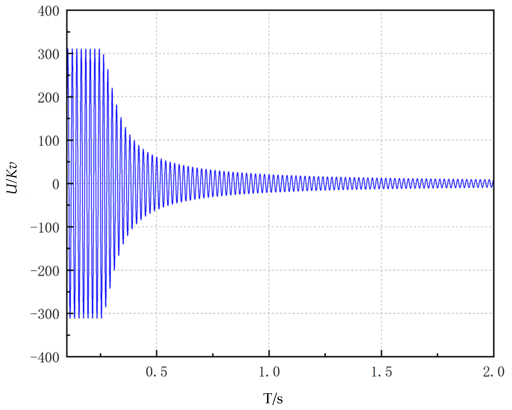
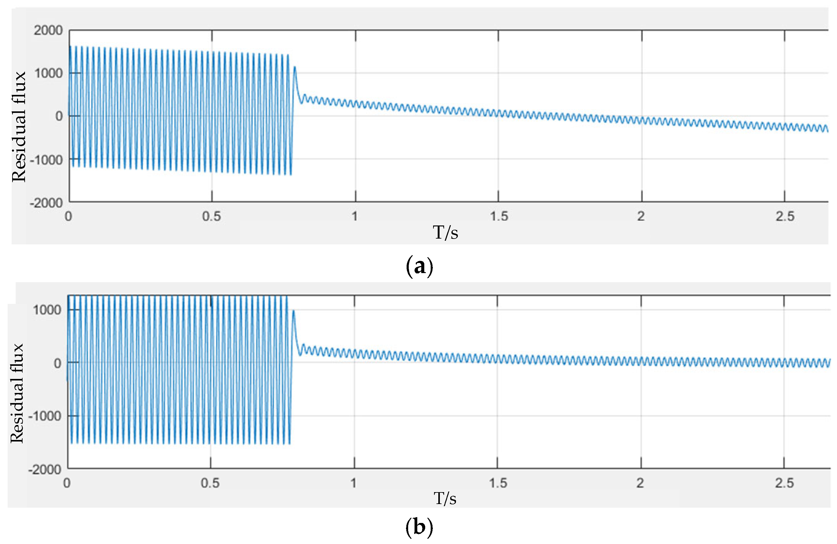
5. Residual Flux Prediction Based on the J-A Model

The effectiveness of conventional controlled switching technology is affected by the residual flux of the transformer. Residual flux is the flux remaining in the core of the transformer after switching off, and the phase at the time of switching off directly affects the magnitude of the residual flux. If other factors are not considered, the calculation formula for residual flux is:

$${\varphi }_r=-{\varphi }_m\cos \left(\omega t_1\right)$$

(18)

In Equation (18), φ_r represents the residual flux in the transformer; φ_m is the peak value of the exciting current; t₁ is the moment when the transformer is switched off; and ω is the angular frequency of the power supply. Equation (18) describes the calculation formula for the residual magnetic flux under ideal conditions, but in actual working conditions, the measurement of residual flux becomes more complex due to the influence of various factors.

When the transformer is operating in no-load conditions, the instantaneous value of the induced electromotive force in the primary winding is:

$$e_1(t)=-N_1{\displaystyle \frac{d\varphi }{dt}}$$

(19)

Let t be the time when the residual flux stabilizes; then, the stabilized residual flux can be expressed as:

$${\varphi }_r=-{\displaystyle \frac{1}{N_1}}{\displaystyle {\int }_{t_0}^{t_{\mathrm{final}}}{e}_1}(t)dt$$

(20)

In theory, the residual flux can be obtained by integrating the voltage across the primary winding of the transformer, but this often results in errors due to the inaccuracy of the upper limit of voltage integration [18]. Factors such as core characteristics and the transient recovery voltage of the circuit breaker cause the residual flux to stabilize over time after switching off. Therefore, the residual flux value obtained by voltage integration at the moment of switching off may have a certain degree of uncertainty. Thus, it is necessary to introduce the J-A model, which can effectively avoid the problem of determining the upper limit of integration in the voltage integration method by judging the residual flux point through the intersection of the hysteresis loop with the ordinate [19].

The measurement method used in this paper is shown in Figure 3. Initially, the voltage and current data of the primary side after the transformer is switched off under no-load conditions are collected and discretized to obtain the discrete data corresponding to the waveforms, as shown in Figure 4 and Figure 5.

The voltage data collected by the voltage acquisition module and the current data collected by the current acquisition module are processed through Equations (21) and (22) to obtain the data for magnetic flux density B and magnetic field strength H.

$$B=-{\displaystyle \frac{1}{N_1}}{\displaystyle {\int }_{t_0}^{t_{\mathrm{final}}}{e}_1}(t)dt$$

(21)

$$H={\displaystyle \frac{N_1\times i(t)}{L_e}}$$

(22)

where i(t) is the instantaneous value of the inrush current, and L_e is the effective magnetic circuit length of the transformer core.

The least-squares method is used to fit the voltage data, taking the absolute value of the voltage and extracting the peak values of each half-cycle after switching off to fit based on the peak data, which allows us to obtain the voltage stabilization time and thus determine t_final. The fitting process is shown in Figure 6. The red circle represents the peak value of the voltage, and the diamond represents the endpoint of the integration. Then, the magnetic flux density and magnetic-field-strength data are used as inputs, and the improved PSO identification algorithm is run once every half-cycle to obtain a dataset of J-A model parameters {M_si, a_i, α_i, k_i, c_i} for i = 1, 2, 3,…, T_max. Finally, the hysteresis loop motion trajectory is generated, and the last intersection of the hysteresis loop with the ordinate is the residual flux point, as shown in Figure 7.

During the process of integrating to obtain the magnetic flux density, the influence of bias magnetization within the core leads to a trend term in the integrated waveform, causing distortion in the real-time magnetic flux density of the core. By employing a polynomial fitting algorithm to identify the order of the trend term contained in the waveform, the aforementioned effects are eliminated, resulting in a stable change in magnetic flux density, as shown in Figure 8.

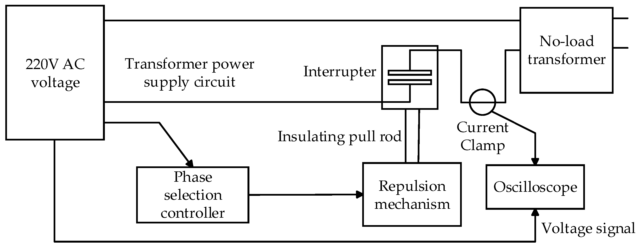
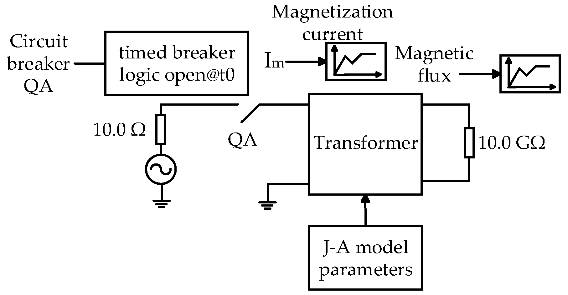
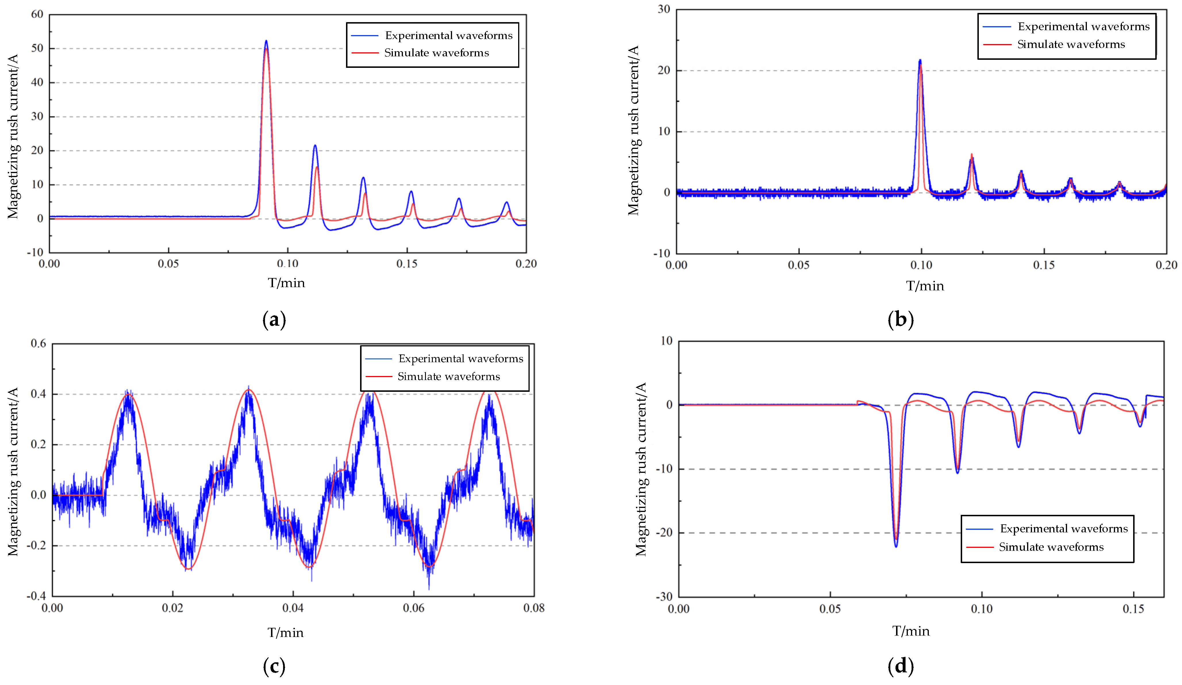
6. Model Simulation and Experimental Validation

Affected by hysteresis, when a transformer operates under no-load conditions, all of the current is used for excitation, and the core is relatively saturated, which can easily reach the saturation state. The waveform and value of the inrush current generated during the no-load switching-on process of the transformer can serve as an important basis for verifying the correctness and accuracy of the residual flux prediction model [20,21,22,23]. The testing platform primarily includes the mains power system, drive circuit, capacitor bank, voltage regulator, phase-selection controller, circuit breaker, single-phase transformer, and various measurement devices. The circuit breaker is a single-phase vacuum circuit breaker, employing a fast-acting and reliable permanent magnet mechanism as its operating mechanism; the capacitor bank drives the circuit breaker to open and close through charging and discharging; after the phase-selection controller issues a trigger signal, it drives the circuit breaker to operate via a thyristor, calculating the closing phase from the residual magnetism and manually inputting it into the controller; a small single-phase transformer serves as the experimental load, with the inrush current during transformer energization captured by a current clamp, and an oscilloscope records the voltage and current signals.

The parameters of the transformer are shown in

Table 3. Transformer parameters.

Parameter	Numerical Value
Rated capacity (VA)	200
Input/Output voltage root mean square (V)	200/160
Copper loss (p.u.)	0.5
Operating frequency (HZ)	50
Eddy-current loss (p.u.)	0.03
Leakage reactance (p.u.)	0.1

, and the experimental circuit diagram is shown in Figure 9.

Meanwhile, a no-load experimental saturation model of the transformer based on the J-A model was constructed using PSCAD 4.6.2 software [24]. The parameters of the J-A model were obtained through a parameter identification algorithm, and the transformer parameters were set according to the actual experiment, with the simulation model depicted in Figure 10. The predicted residual flux values were input into the transformer model. In the experiment, both the actual and simulated circuit breakers were closed at the same angle to detect the peak of the inrush current, and the accuracy of the residual flux value predicted by the J-A model was verified by the magnitude of the error.

Different closing angles can be obtained through controlled switching technique. A comparison of simulation results with experimental results is shown in

Table 4. Peak value of inrush current in each waveform.

Exciting Inrush Current Peak	30°	60°	90°	120°
Simulation results (A)	50.006	20.961	0.400	−20.972
Experimental results (A)	52.422	21.818	0.420	−22.183
Relative error (%)	4.8	3.9	4.8	5.5

and Figure 11.

From the above figures and table results, it can be seen that the peak value of the inrush current within the first cycle after the circuit breaker closes is very close to the results obtained from the simulation model, which verifies the accuracy of the parameter identification algorithm. At the same time, the accuracy and effectiveness of predicting transformer residual flux based on J-A theory have also been validated.

7. Conclusions and Future Studies

The residual flux can be calculated using the J-A hysteresis model. This method is capable of computing the hysteresis loop information following the no-load switching off of the transformer and obtaining accurate residual flux values, overcoming the issue of inaccuracy calculation due to the imprecise determination of the upper limit of integration in the voltage integration method.

In the process of parameter identification for the J-A model, the particle-swarm optimization (PSO) algorithm was improved by optimizing the velocity and position-update formulas for the particles. This algorithm has the advantages of not easily falling into local optima, rapid convergence, and high parameter identification accuracy. It has improved the precision and speed of residual flux calculation. On this basis, the J-A model established in this article can also be used to calculate the hysteresis loss of iron core materials in high-voltage motors and generators, help optimize motor efficiency, and assist in the design of high-performance reactors.

Through simulation and experimental validation, by comparing the peak values of inrush current under different no-load closing angles after the transformer is switched off, the calculation method based on the J-A hysteresis model can accurately determine the residual flux. To further improve the accuracy of remanence prediction, more complex deep learning architectures can be explored to capture the time-series features and nonlinear relationships of remanence [25,26]. High-precision sensors can be developed to collect real-time operational status data of transformers and input it into predictive models. In addition, uncertainty analysis methods can be introduced to evaluate the reliability of prediction results.

References

1. Nasution, M.F.; Mustafa, F.; Shaulgara, S. Case studies of magnetizing inrush current effect on differential & REF transformer protection. In Proceedings of the 2019 2nd International Conference on High Voltage Engineering and Power Systems (ICHVEPS), Denpasar, Indonesia, 1–4 October 2019; pp. 1–6. [Google Scholar]
2. Zhijiang, L.; Xuehua, L.; ShuYong, L.; Libin, H. Study on the excitation inrush suppression strategy of phase-selective switching converter with closing resis-tor switch considering dispersion. In Proceedings of the 2022 China International Conference on Electricity Distribution (CICED), Changsha, China, 7–8 September 2022; pp. 1280–1285. [Google Scholar]
3. Sung, B.C.; Kim, S. Accurate transformer inrush current analysis by controlling closing instant and residual flux. Electr. Power Syst. Res. 2023, 223, 109638. [Google Scholar] [CrossRef]
4. Hamilton, R. Analysis of transformer inrush current and comparison of harmonic restraint methods in transformer protection. IEEE Trans. Ind. Appl. 2013, 49, 1890–1899. [Google Scholar] [CrossRef]
5. Komarzyniec, G. Calculating the inrush current of superconducting transformers. Energies 2021, 14, 6714. [Google Scholar] [CrossRef]
6. Yonezawa, R. Development of a reversible transformer model for the calculation of inrush currents energizing from higher and lower voltage windings. Electr. Eng. Jpn. 2022, 215, e23365. [Google Scholar] [CrossRef]
7. Xie, W.; Xiao, F.; Tu, C.; Zheng, Y.; Peng, Z.; Guo, Q. Suppression strategy for the inrush current of a solid-state transformer caused by the reclosing process. Prot. Control Mod. Power Syst. 2023, 8, 53. [Google Scholar] [CrossRef]
8. Ge, Y.; Zheng, J.; Ren, X.; Chen, S.; Kong, X.; Wang, C. Preventing maloperation scheme for saturation protection of converter transformers based on waveform prediction of magnetizing inrush current. Electr. Eng. 2024, 1–14. [Google Scholar] [CrossRef]
9. Guoying, L.; Qiang, S.; Lingyun, W.; Dingqu, Z.; Feng, P. A hybrid algorithm based on fish swarm and simulated annealing for parameters identification of modified JA model. In Proceedings of the 2017 13th IEEE International Conference on Electronic Measurement & Instruments (ICEMI), Yangzhou, China, 20–22 October 2017; pp. 483–488. [Google Scholar]
10. Zhu, X.; Shen, S.; Zhang, G.; Wang, Z. An Improved Method for Parameter Identification of JA Models. In Proceedings of the 2024 7th International Conference on Electronics Technology (ICET), Chengdu, China, 17–20 May 2024; pp. 1151–1155. [Google Scholar]
11. Das, S.; Santra, T.; Choudhury, A.B.; Roy, D.; Yamada, S. Transient modeling and performance analysis of a passive magnetic fault current limiter considering JA hysteresis model. Electr. Power Compon. Syst. 2019, 47, 396–405. [Google Scholar] [CrossRef]
12. Lu, H.-l.; Wen, X.-s.; Lan, L.; An, Y.-z.; Li, X.-p. A self-adaptive genetic algorithm to estimate JA model parameters considering minor loops. J. Magn. Magn. Mater. 2015, 374, 502–507. [Google Scholar]
13. Zhang, D.; Sha, D.; Gao, C.; Liu, X.; Long, H.; Tang, G.; Zhao, Y.; Gao, Y. A Closed-Loop Soft Startup Strategy to Suppress Inrush Current for Full-Bridge Modular Multilevel Converters. IEEE Trans. Power Electron. 2024, 39, 14787–14799. [Google Scholar]
14. Key, S.; Son, G.-W.; Nam, S.-R. Deep Learning-Based Algorithm for Internal Fault Detection of Power Transformers during Inrush Current at Distribution Substations. Energies 2024, 17, 963. [Google Scholar] [CrossRef]
15. Pham, M.-T.; Zhang, D.; Koh, C.S. Multi-guider and cross-searching approach in multi-objective particle swarm optimization for electromagnetic problems. IEEE Trans. Magn. 2012, 48, 539–542. [Google Scholar] [CrossRef]
16. Coelho, L.d.S.; Guerra, F.A.; Leite, J.V. Multiobjective exponential particle swarm optimization approach applied to hysteresis parameters estimation. IEEE Trans. Magn. 2012, 48, 283–286. [Google Scholar] [CrossRef]
17. Zhang, Q.; Xie, Z.; Lu, M.; Ji, S.; Liu, D.; Xiao, Z. Optimization of Hydropower Unit Startup Process Based on the Improved Multi-Objective Particle Swarm Optimization Algorithm. Energies 2024, 17, 4473. [Google Scholar] [CrossRef]
18. Mohammadpour, H.; Dashti, R.; Shaker, H.R. A new practical approach for discrimination between inrush currents and internal faults in power transformers. Technol. Econ. Smart Grids Sustain. Energy 2020, 5, 5. [Google Scholar]
19. Sima, W.; Zou, M.; Yang, M.; Peng, D.; Liu, Y. Saturable reactor hysteresis model based on Jiles–Atherton formulation for ferroresonance studies. Int. J. Electr. Power Energy Syst. 2018, 101, 482–490. [Google Scholar]
20. Cardelli, E.; Faba, A.; Tissi, F. Prediction and control of transformer inrush currents. IEEE Trans. Magn. 2015, 51, 1–4. [Google Scholar] [CrossRef]
21. Li, C.; Yang, Y.; Li, W.; Li, H. A soft-start-based method for active suppression of magnetizing inrush current in transformers. Electronics 2023, 12, 3114. [Google Scholar] [CrossRef]
22. Yu, S.; Li, Y.; Yu, Z.; Wang, X.; Li, P. Calculation of Transformer Reclosing Short Circuit Strength Considering the Influence of Remanent Magnetism. In Proceedings of the 2023 IEEE International Conference on Applied Superconductivity and Electromagnetic Devices (ASEMD), Tianjin, China, 27–29 October 2023; pp. 1–2. [Google Scholar]
23. Łukaniszyn, M.; Majka, Ł.; Baron, B.; Kulesz, B.; Tomczewski, K.; Wróbel, K. Measurement Verification of a Developed Strategy of Inrush Current Reduction for a Non-Loaded Three-Phase Dy Transformer. Energies 2024, 17, 5368. [Google Scholar] [CrossRef]
24. Zhou, P.; Xiang, Z.; Wang, D.; Ban, L.; Ding, L.; Wei, W. Methods for Obtaining Excitation Curves and Residual flux of Transformers by De-energizing and Energizing Test. In Proceedings of the 2019 IEEE 3rd International Electrical and Energy Conference (CIEEC), Beijing, China, 7–9 September 2019; pp. 716–720. [Google Scholar]
25. Gbadega, P.A.; Saha, A.K. Impact of incorporating disturbance prediction on the performance of energy management systems in micro-grid. IEEE Access 2020, 8, 162855–162879. [Google Scholar] [CrossRef]
26. García, D.; Herrera, M.; Camacho, O. A Comparative Evaluation of Metaheuristic Optimization Methods for Control Applications. In Proceedings of the 2023 IEEE Seventh Ecuador Technical Chapters Meeting (ECTM), Ambato, Ecuador, 10–13 October 2023; pp. 1–6. [Google Scholar]
Figure 1. Comparison of results of different parameter identification algorithms.
Energies 18 01631 g001
Figure 2. The variation in RMSE of each algorithm with the number of iterations.
Energies 18 01631 g002
Figure 3. Calculation process of residual flux.
Energies 18 01631 g003
Figure 4. Waveform of no-load opening voltage of transformer.
Energies 18 01631 g004
Figure 5. Waveform of inrush current for no-load opening of transformer.
Energies 18 01631 g005
Figure 6. Principle of least-squares processing.
Energies 18 01631 g006
Figure 7. Change in magnetic flux during voltage integration process.
Energies 18 01631 g007
Figure 8. Correcting distorted residual flux waveforms. (a) Original residual flux density waveform. (b) Residual flux density waveform after demagnetization.
Energies 18 01631 g008
Figure 9. Circuit diagram of transformer no-load test.
Energies 18 01631 g009
Figure 10. Simulation model.
Energies 18 01631 g010
Figure 11. Comparison of inrush current waveforms at different closing angles. (a) At a closing angle of 30° and a residual flux of −0.2 p.u. (b) At a closing angle of 60° and a residual flux of 0.09 p.u. (c) At a closing angle of 90° and a residual flux of −0.1 p.u. (d) At a closing angle of 120° and a residual flux of 0.3 p.u.
Energies 18 01631 g011