
S-Transform Based Time–Frequency Evaluation of Dynamic Stray Current in Zero-Resistance Converter System

Abstract
1. Introduction
2. Traction Power Supply System and ZRCS
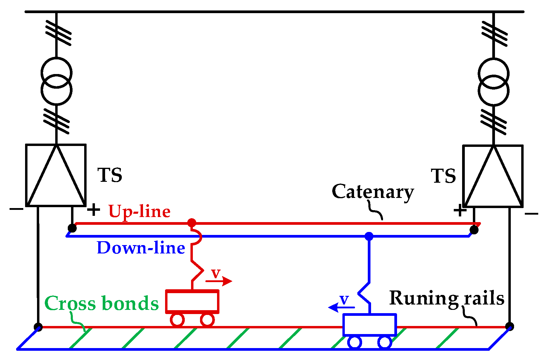
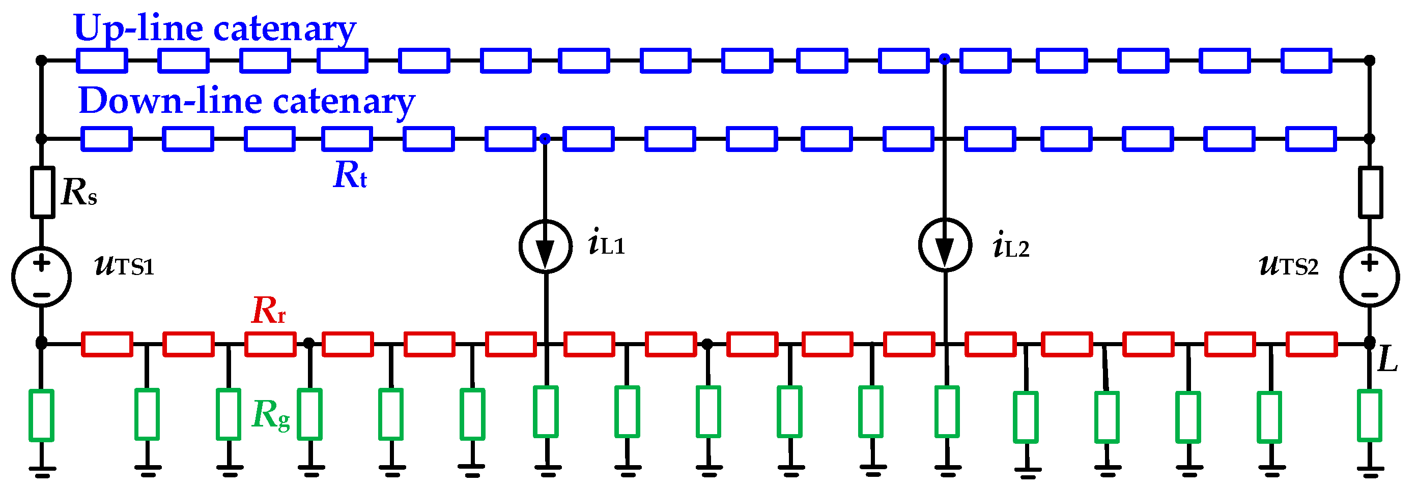
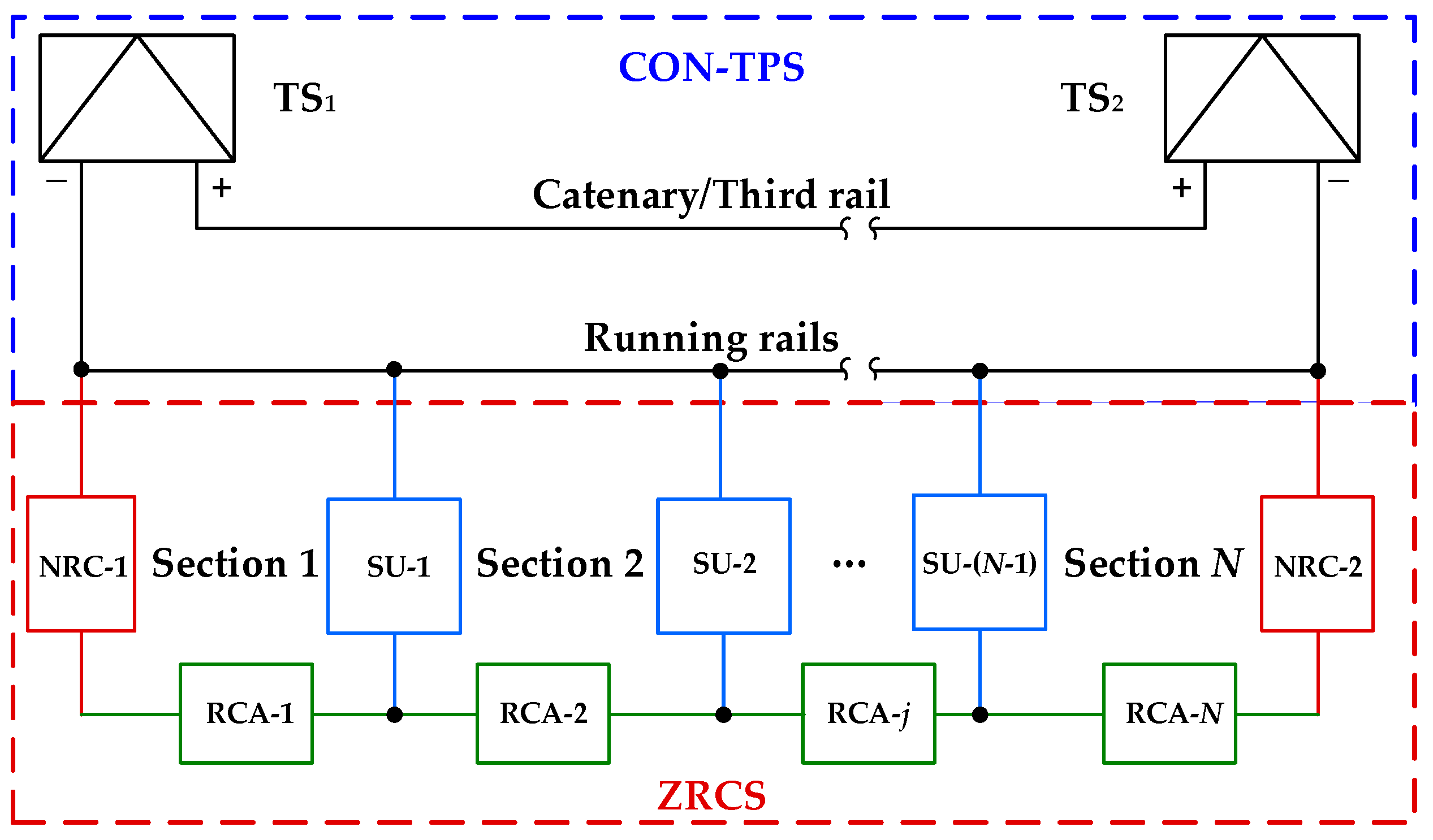
2.1. Traction Power Supply System
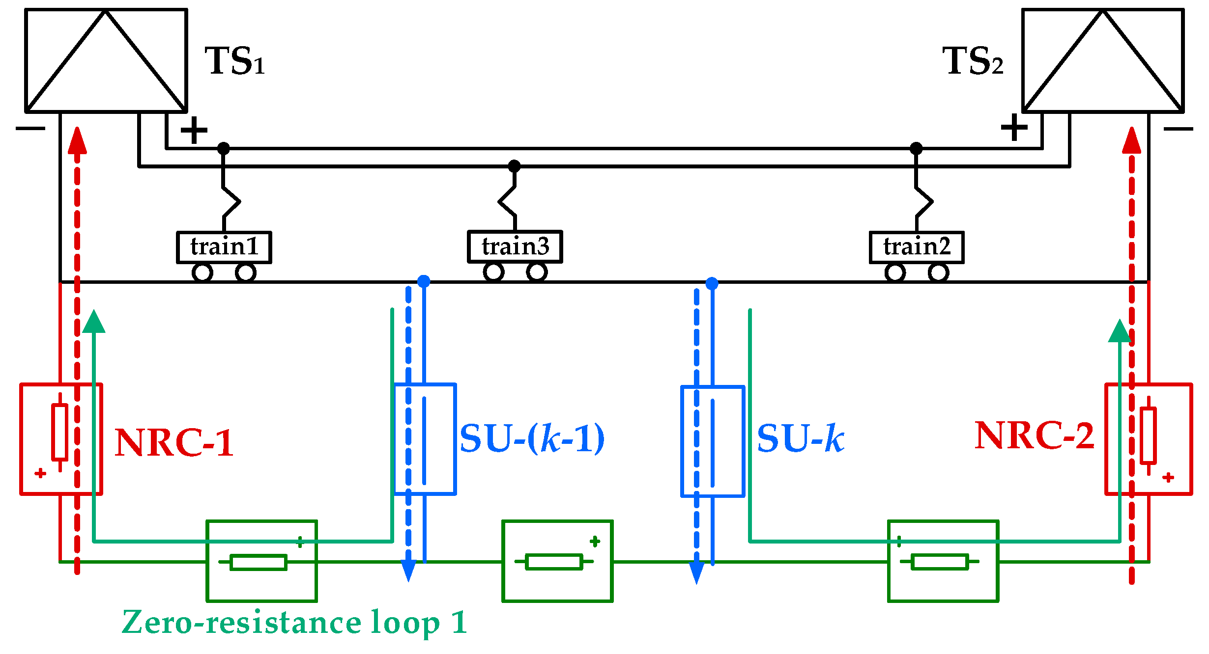
2.2. Configuration and Control Strategy of ZRCS
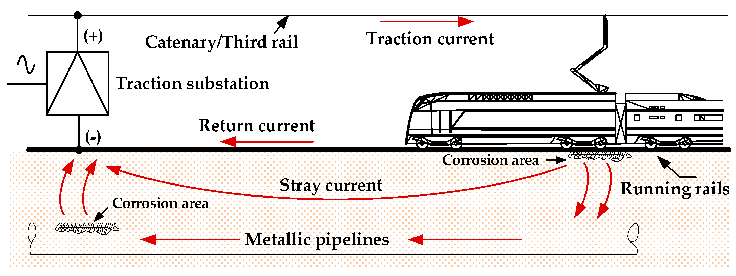
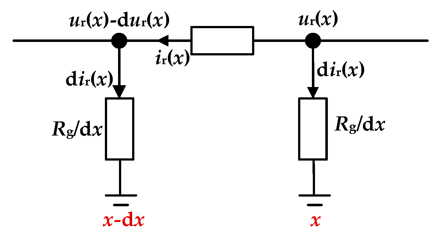
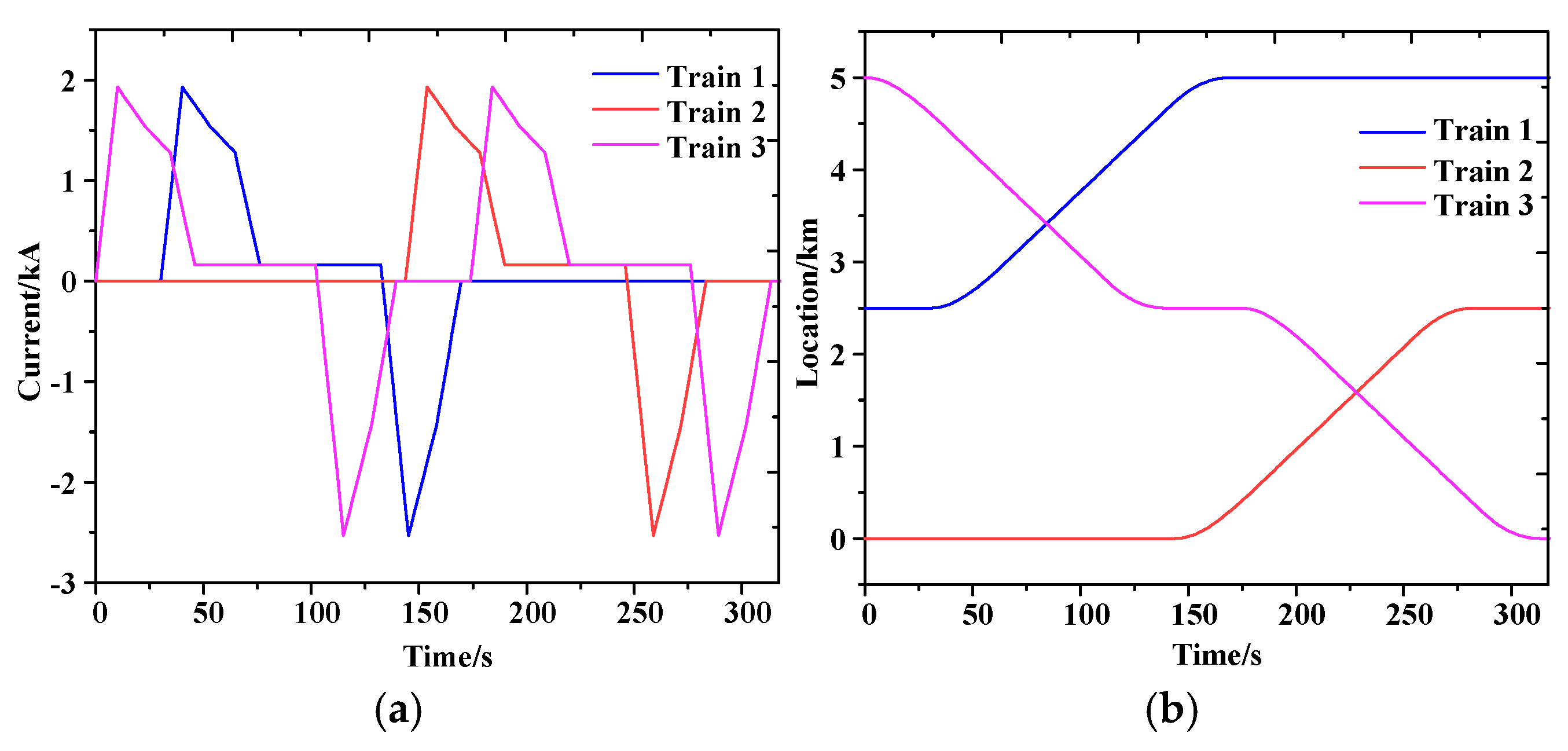
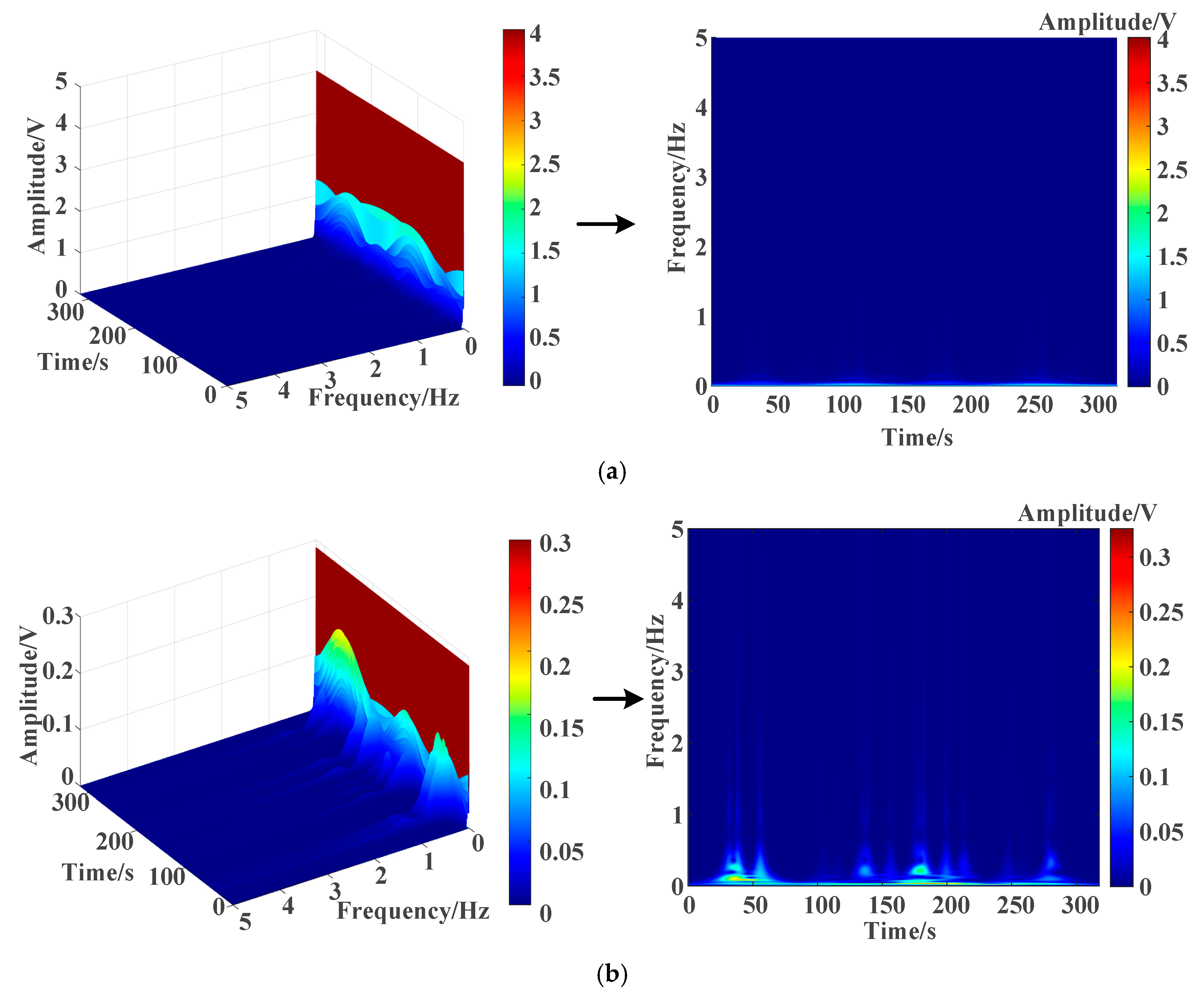
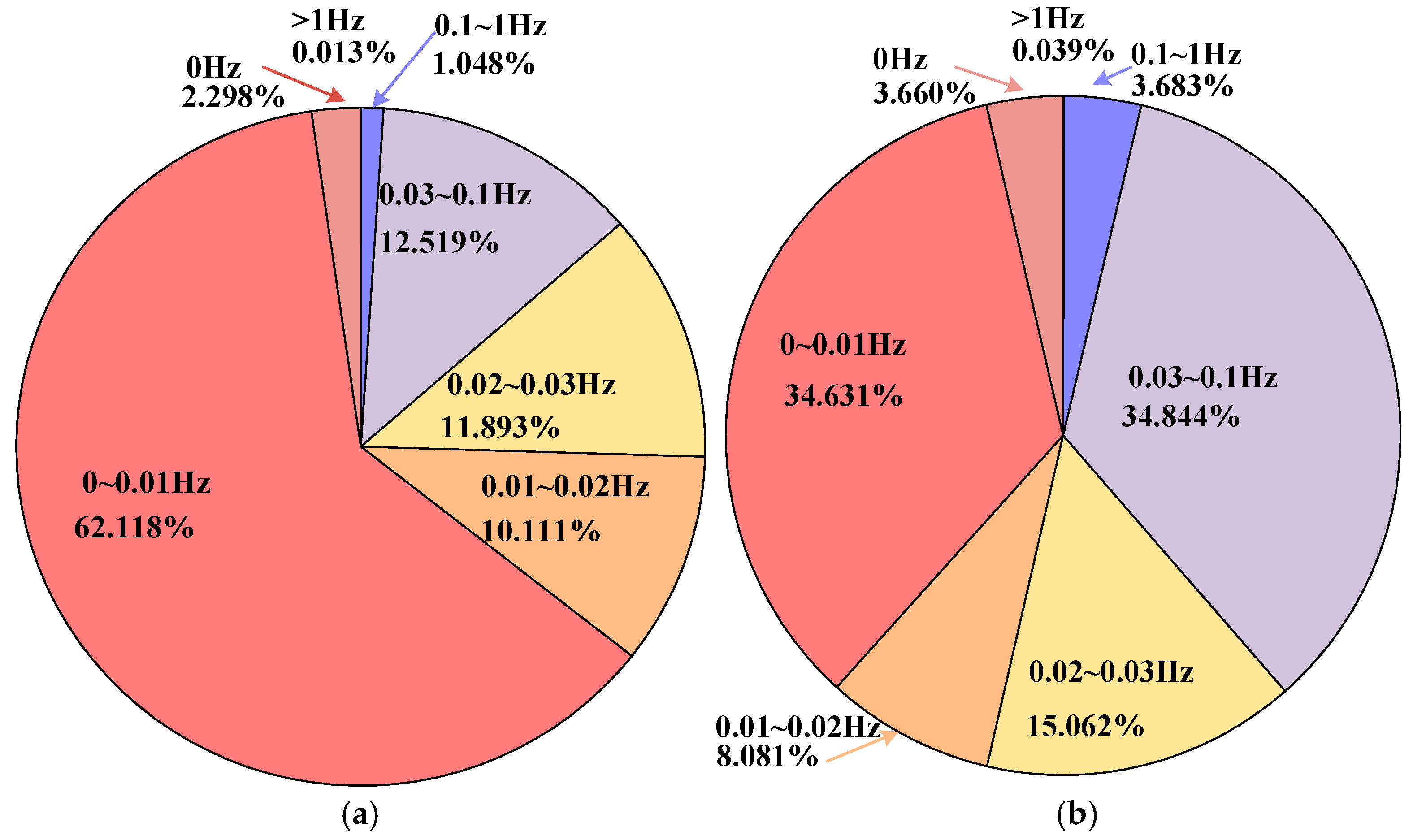
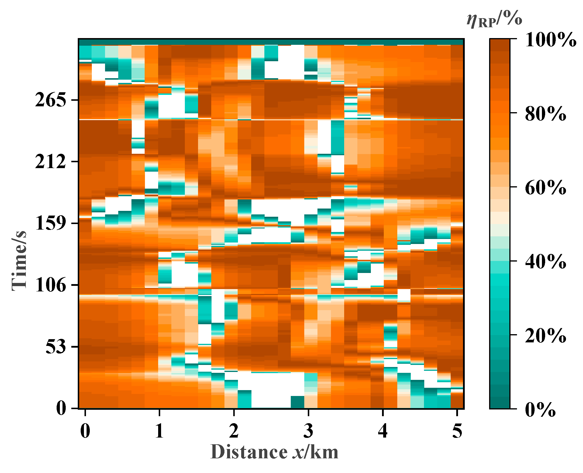
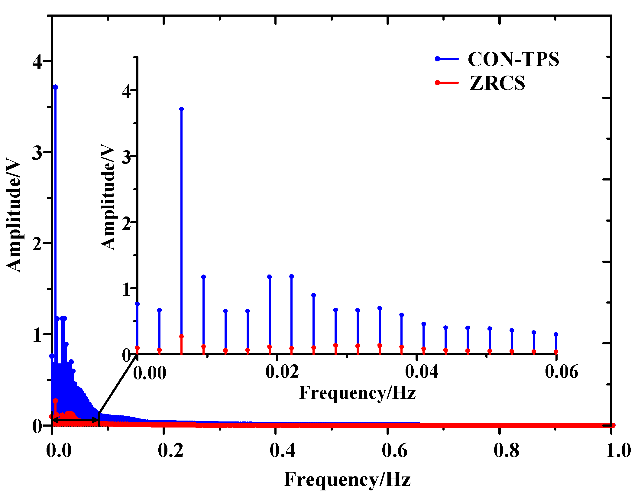
3. Time–Frequency Analysis of Stray Current
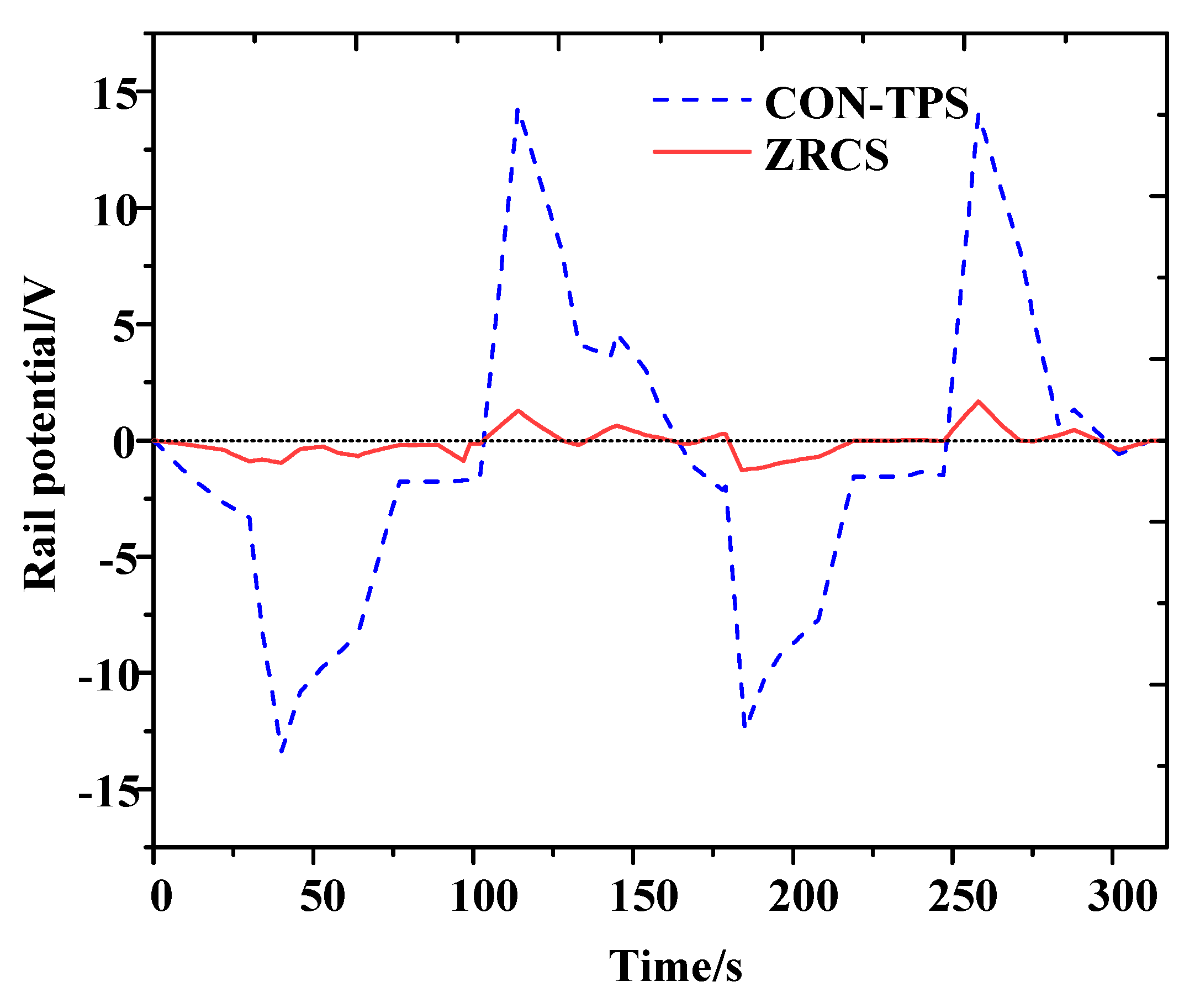
4. Evaluation of Rail Potential and Stray Current
5. Experimental Verifications
6. Conclusions
Author Contributions
Funding
Data Availability Statement
Conflicts of Interest
References
- Han, B.; Yu, Y.; Xi, Z.; Sun, Y.; Lu, F.; Li, S.; Li, Z.; Huang, S.; Hu, J.; Sang, Y.; et al. Statistical Analysis of Urban Rail Transit Operations Worldwide in 2023: A Review. Urban Rapid Rail Transit 2024, 37, 1–9. [Google Scholar]
- Hu, J.; Yang, M.; Zhen, Y. A Review of Resilience Assessment and Recovery Strategies of Urban Rail Transit Networks. Sustainability 2024, 16, 6390. [Google Scholar] [CrossRef]
- Dolara, A.; Foiadelli, F.; Leva, S. Stray Current Effects Mitigation in Subway Tunnels. IEEE Trans. Power Deliv. 2012, 27, 2304–2311. [Google Scholar] [CrossRef]
- Yang, X.; Wang, M.; Zheng, T.Q.; Sun, X. Modelling and Simulation of Stray Current in Urban Rail Transit—A Review. Urban Rail Transit 2024, 10, 189–199. [Google Scholar] [CrossRef]
- Zaboli, A.; Vahidi, B.; Yousefi, S.; Hosseini-Biyouki, M.M. Evaluation and Control of Stray Current in DC-Electrified Railway Systems. IEEE Trans. Veh. Technol. 2017, 66, 974–980. [Google Scholar] [CrossRef]
- Chen, Z.; Koleva, D.; van Breugel, K. A review on stray current-induced steel corrosion in infrastructure. Corros. Rev. 2017, 35, 397–423. [Google Scholar] [CrossRef]
- Du, G.; Wang, J.; Jiang, X.; Zhang, D.; Yang, L.; Hu, Y. Evaluation of Rail Potential and Stray Current with Dynamic Traction Networks in Multitrain Subway Systems. IEEE Trans. Transp. Electrif. 2020, 6, 784–796. [Google Scholar] [CrossRef]
- Ogunsola, A.; Sandrolini, L.; Mariscotti, A. Evaluation of Stray Current From a DC-Electrified Railway with Integrated Electric-Electromechanical Modeling and Traffic Simulation. IEEE Trans. Ind. Appl. 2015, 51, 5431–5441. [Google Scholar] [CrossRef]
- Wang, M.; Yang, X.; Zheng, T.Q.; Ni, M. DC Autotransformer-Based Traction Power Supply for Urban Transit Rail Potential and Stray Current Mitigation. IEEE Trans. Transp. Electrif. 2020, 6, 762–773. [Google Scholar] [CrossRef]
- Stray Current Corrosion in Electrified Rail Systems—Final Report. Available online: https://rosap.ntl.bts.gov/view/dot/13213 (accessed on 17 February 2025).
- Qin, H.; Du, Y.; Lu, M.; Meng, Q. Effect of dynamic DC stray current on corrosion behavior of X70 steel. Mater. Corros. -Werkst. Und Korros. 2020, 71, 35–53. [Google Scholar] [CrossRef]
- Darowicki, K.; Zakowski, K. A new time-frequency detection method of stray current field interference on metal structures. Corros. Sci. 2004, 46, 1061–1070. [Google Scholar] [CrossRef]
- Mujezinovic, A.; Martinez, S. Application of the Continuous Wavelet Cross-Correlation Between Pipe-to-Soil Potential and Pipe-to-Rail Voltage Influenced by Dynamic Stray Current from DC Train Traction. IEEE Trans. Power Deliv. 2021, 36, 1015–1023. [Google Scholar] [CrossRef]
- Stockwell, R.G.; Mansinha, L.; Lowe, R.P. Localization of the complex spectrum: The S transform. IEEE Trans. Signal Process. 1996, 44, 998–1001. [Google Scholar] [CrossRef]
- Wang, Y.-Q.; Li, W.; Yang, X.-F.; Ye, G.; Fan, Q.-G.; Zhang, L.-P. Study on the Distribution and Computer Simulation of Metro Rail Potential. In Proceedings of the International Conference on Informatics, Cybernetics, and Computer Engineering (ICCE2011), Cybernetics, MEL, Australia, 19–20 November 2011; pp. 185–192. [Google Scholar]
- Vranesic, K.; Bhagat, S.; Mariscotti, A.; Vail, R. Measures and Prescriptions to Reduce Stray Current in the Design of New Track Corridors. Energies 2023, 16, 6252. [Google Scholar] [CrossRef]
- Ha, T.H.; Bae, J.H.; Lee, H.G.; Ha, Y.C.; Kim, D.K. Rapid potential-controlled rectifier for securing the underground pipeline under electrolytic interference. In Proceedings of the International Conference on Power System Technology (POWERCON 2004), Singapore, 21–24 November 2004; pp. 537–541. [Google Scholar]
- Trykoz, L.; Kamchatnaya, S.; Borodin, D.; Atynian, A.; Tkachenko, R. Protection of railway infrastructure objects against electrical corrosion. Anti-Corros. Methods Mater. 2021, 68, 380–384. [Google Scholar] [CrossRef]
- Wang, A.; Lin, S.; Hu, Z.; Li, J.; Wang, F.; Wu, G.; He, Z. Evaluation Model of DC Current Distribution in AC Power Systems Caused by Stray Current of DC Metro Systems. IEEE Trans. Power Deliv. 2021, 36, 114–123. [Google Scholar] [CrossRef]
- Machczyñski, W. Simulation model for drainage protection of earth-return circuits laid in stray currents area. Electr. Eng. 2002, 84, 165–172. [Google Scholar] [CrossRef]
- Rossouw, E.; Doorsamy, W. Predictive Maintenance Framework for Cathodic Protection Systems Using Data Analytics. Energies 2021, 14, 5805. [Google Scholar] [CrossRef]
- Gu, J.; Yang, X.; Zheng, T.Q.; Xia, X.; Zhao, Z.; Chen, M. Rail Potential and Stray Current Mitigation for Urban Rail Transit with Multiple Trains Under Multiple Conditions. IEEE Trans. Transp. Electrif. 2022, 8, 1684–1694. [Google Scholar] [CrossRef]
- Chen, M.; Yang, X.; Zheng, T.Q.; Zhao, Z.; Xia, X.; Gu, J. Improved control strategy of zero-resistance converter system for rail potential and stray current mitigation. Int. J. Rail Transp. 2023, 11, 248–266. [Google Scholar] [CrossRef]
- Zakowski, K.; Sokolski, W. 24-hour characteristic of interaction on pipelines of stray currents leaking from tram tractions. Corros. Sci. 1999, 41, 2099–2111. [Google Scholar] [CrossRef]
- Samantaray, S.R.; Tripathy, L.N.; Dash, P.K. Differential energy based relaying for thyristor controlled series compensated line. Int. J. Electr. Power Energy Syst. 2012, 43, 621–629. [Google Scholar] [CrossRef]


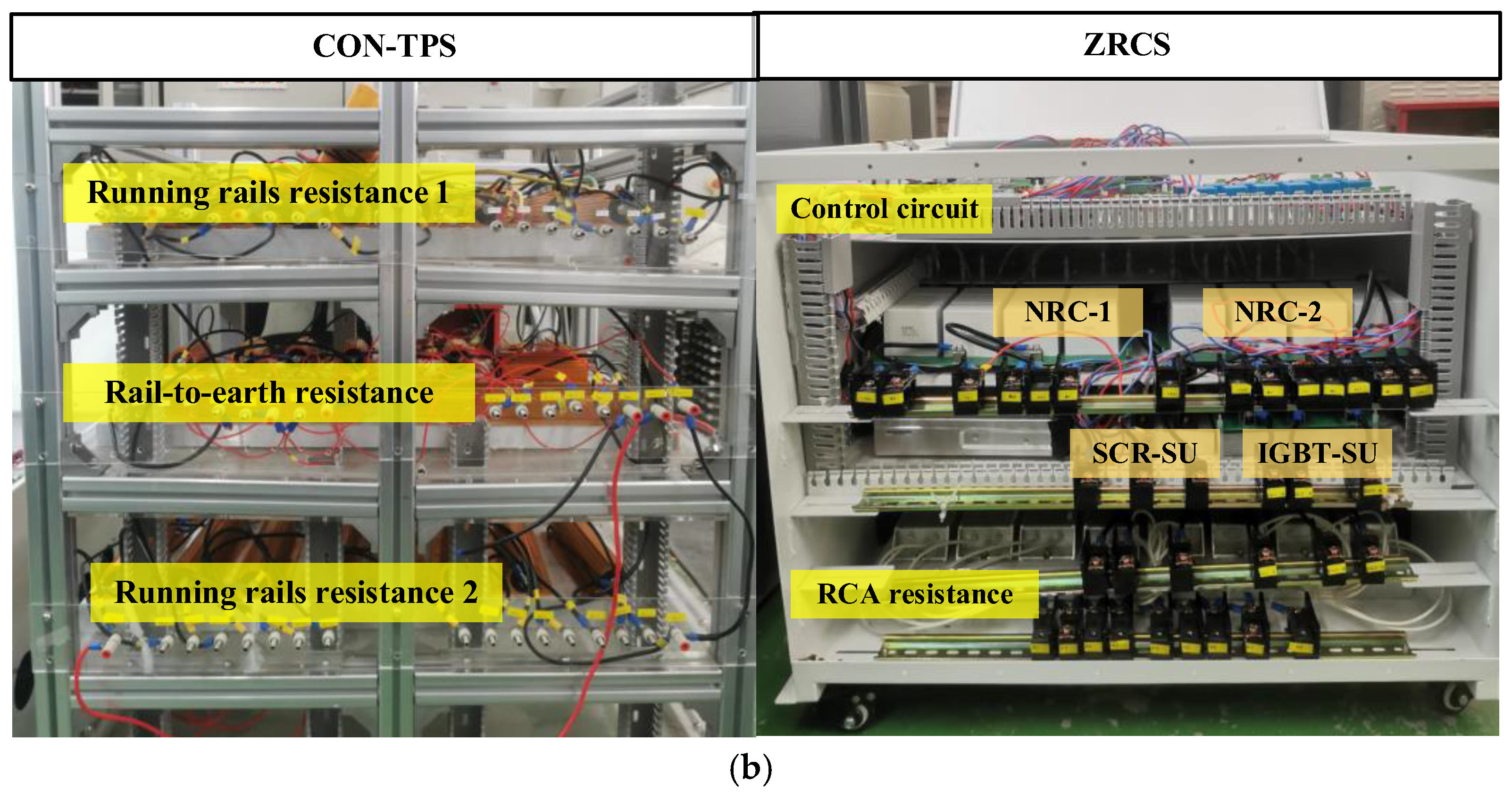
| Variable | Description | Value |
|---|---|---|
| Rg | Rail-to-earth resistance | 15 Ω•km |
| Rr | Running rails resistance | 10 mΩ/km |
| Rt | Catenary resistance | 10 mΩ/km |
| RRca | RCA resistance | 24 mΩ/km |
| Rs | Equivalent internal resistance of TS | 1.5 mΩ |
| L | Distance between TSs | 5 km |
| N | Rail-section quantity | 4 |
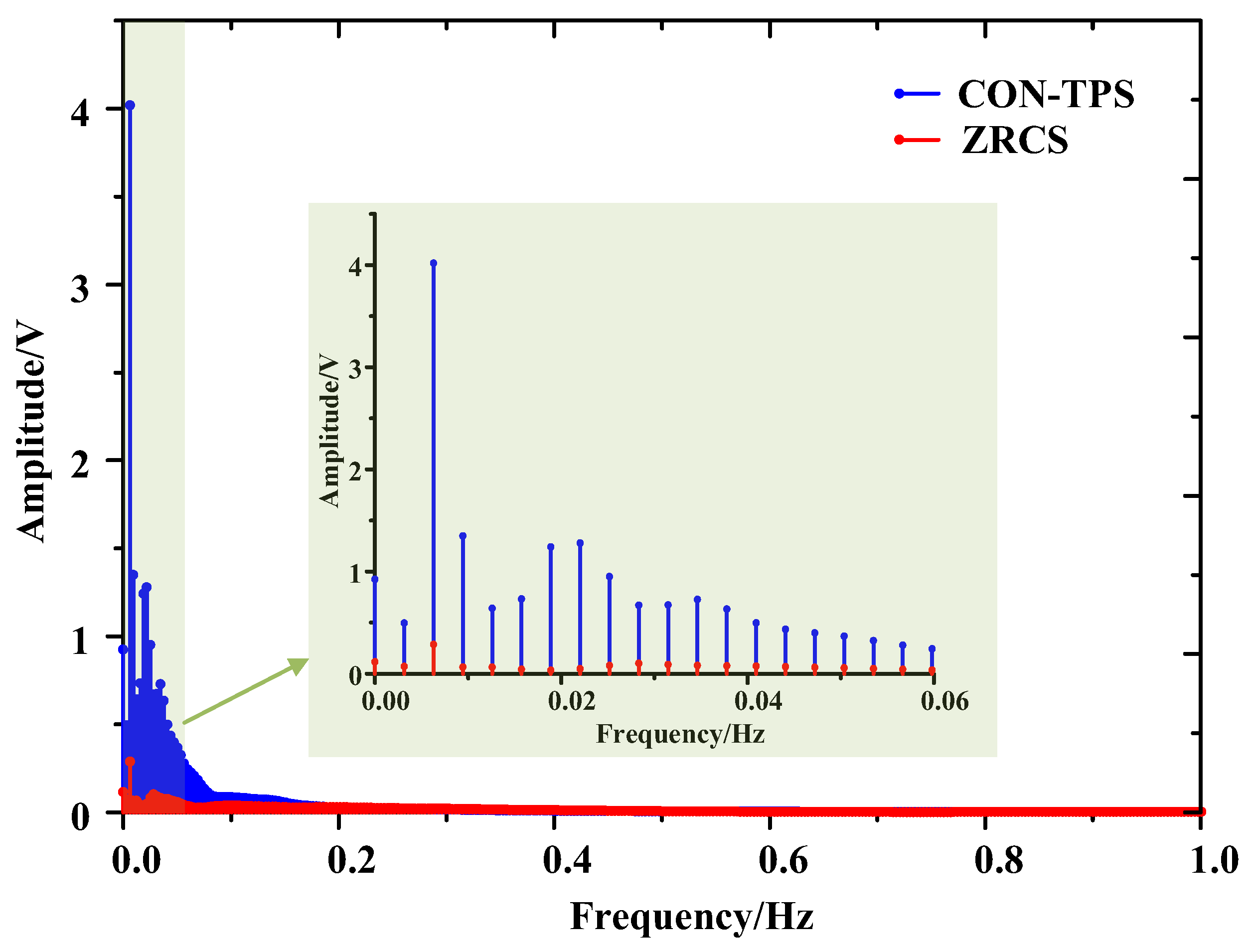
| System | Maximum Rail Potential at TS1 | Minimum Rail Potential at TS1 | Maximum Amplitude | Ratio of 0–0.03 Hz |
|---|---|---|---|---|
| CON-TPS | 15.13 V | −14.19 V | 4.02 V | 88.70% |
| ZRCS | 1.12 V | −2.59 V | 0.326 V | 35.04% |
| Variable | Description | Value |
|---|---|---|
| Rg | Rail-to-earth resistance | 15 Ω•km |
| Rr | Running rails resistance | 1.6 Ω/km |
| RRca | RCA resistance | 0.8 Ω/km |
| Rs | Equivalent internal resistance of TS | 0.2 Ω |
| L | Distance between TSs | 5 km |
| N | Rail-section quantity | 4 |
| System | Maximum Rail Potential at TS1 | Minimum Rail Potential at TS1 | Maximum Amplitude | Ratio of 0–0.03 Hz |
|---|---|---|---|---|
| CON-TPS | 14.03 V | −13.37 V | 3.72 V | 86.49% |
| ZRCS | 1.66 V | −1.27 V | 0.27 V | 61.48% |
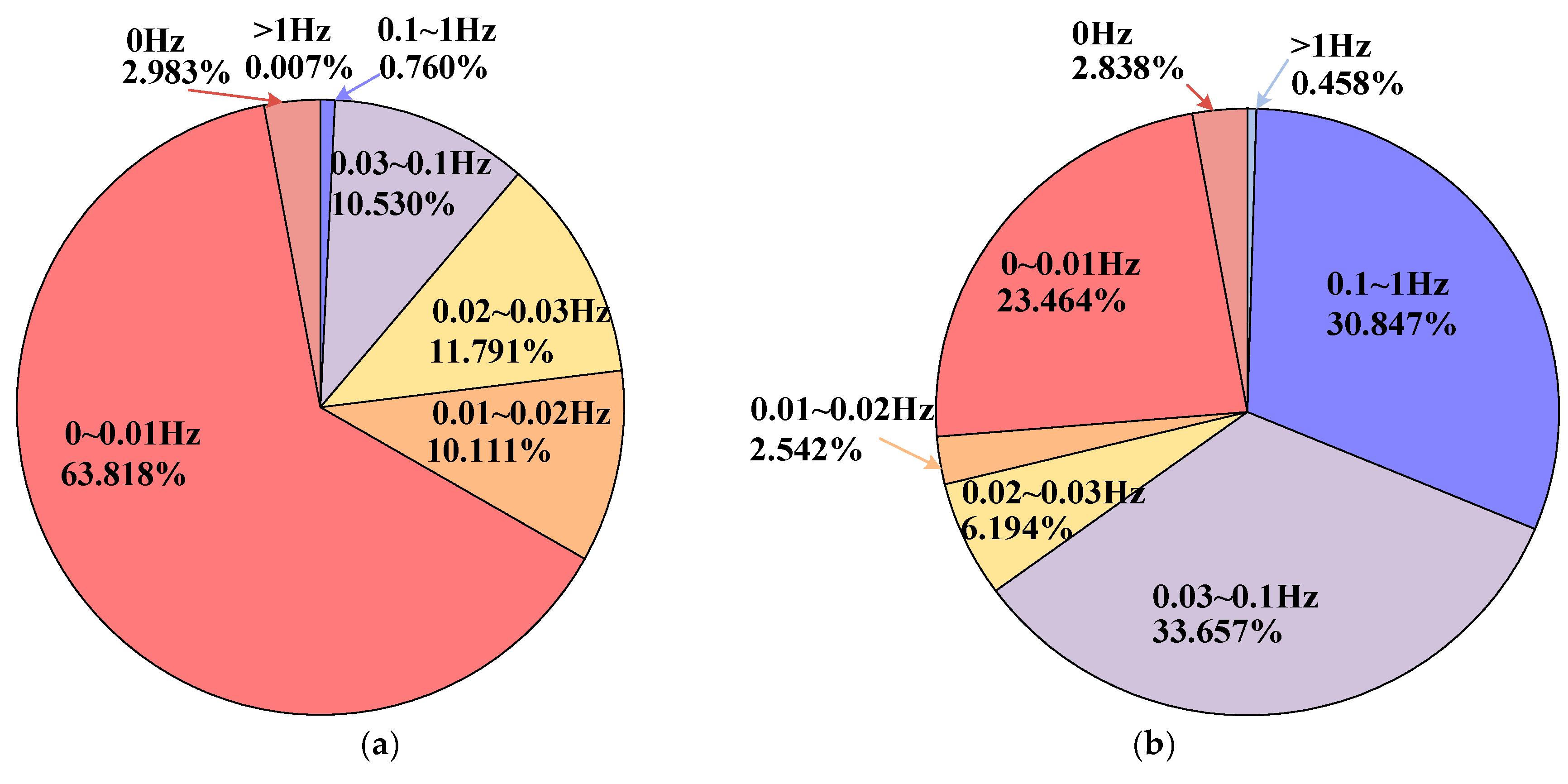
| System | 0–0.03 Hz | 0.03–0.1 Hz | 0.1–1 Hz | |
|---|---|---|---|---|
| Simulation | CON-TPS | 88.70% | 10.53% | 0.76% |
| ZRCS | 35.04% | 33.66% | 30.85% | |
| Experiment | CON-TPS | 86.49% | 12.52% | 1.05% |
| ZRCS | 61.48% | 34.84% | 3.68% |
Disclaimer/Publisher’s Note: The statements, opinions and data contained in all publications are solely those of the individual author(s) and contributor(s) and not of MDPI and/or the editor(s). MDPI and/or the editor(s) disclaim responsibility for any injury to people or property resulting from any ideas, methods, instructions or products referred to in the content. |
© 2025 by the authors. Licensee MDPI, Basel, Switzerland. This article is an open access article distributed under the terms and conditions of the Creative Commons Attribution (CC BY) license (https://creativecommons.org/licenses/by/4.0/).
Share and Cite
Sun, X.; Yang, X.; Zhao, R.; Wang, Z.; Chen, M.; Zheng, T.Q. S-Transform Based Time–Frequency Evaluation of Dynamic Stray Current in Zero-Resistance Converter System. Energies 2025, 18, 1594. https://doi.org/10.3390/en18071594
Sun X, Yang X, Zhao R, Wang Z, Chen M, Zheng TQ. S-Transform Based Time–Frequency Evaluation of Dynamic Stray Current in Zero-Resistance Converter System. Energies. 2025; 18(7):1594. https://doi.org/10.3390/en18071594
Chicago/Turabian StyleSun, Xiangxuan, Xiaofeng Yang, Runda Zhao, Zhenshuai Wang, Maolu Chen, and Trillion Q. Zheng. 2025. "S-Transform Based Time–Frequency Evaluation of Dynamic Stray Current in Zero-Resistance Converter System" Energies 18, no. 7: 1594. https://doi.org/10.3390/en18071594
APA StyleSun, X., Yang, X., Zhao, R., Wang, Z., Chen, M., & Zheng, T. Q. (2025). S-Transform Based Time–Frequency Evaluation of Dynamic Stray Current in Zero-Resistance Converter System. Energies, 18(7), 1594. https://doi.org/10.3390/en18071594