Article

An Evaluation of the Power System Stability for a Hybrid Power Plant Using Wind Speed and Cloud Distribution Forecasts

by
Théodore Desiré Tchokomani Moukam
1,*,
Akira Sugawara
2,
Yuancheng Li
1 and
Yakubu Bello
1
1
Graduate School of Science and Technology, Niigata University, Niigata 950-2181, Japan
2
Department of Electrical and Electronic Engineering, Faculty of Engineering, Niigata University, 8050 Ikarashi-2, Niigata 950-2181, Japan
*
Author to whom correspondence should be addressed.
Energies 2025, 18(6), 1540; https://doi.org/10.3390/en18061540
Submission received: 30 January 2025 / Revised: 17 March 2025 / Accepted: 18 March 2025 / Published: 20 March 2025
(This article belongs to the Section F1: Electrical Power System)

Abstract

:
Power system stability (PSS) refers to the capacity of an electrical system to maintain a consistent equilibrium between the generation and consumption of electric power. In this paper, the PSS is evaluated for a “hybrid power plant” (HPP) which combines thermal, wind, solar photovoltaic (PV), and hydropower generation in Niigata City. A new method for estimating its PV power generation is also introduced based on NHK (the Japan Broadcasting Corporation)’s cloud distribution forecasts (CDFs) and land ratio settings. Our objective is to achieve frequency stability (FS) while reducing CO2 emissions in the power generation sector. So, the PSS is evaluated according to the results in terms of the FS variable. Six-minute autoregressive wind speed prediction (6ARW) support is used for wind power (WP). One-hour GPV wind farm (1HWF) power is computed from the Grid Point Value (GPV) wind speed prediction data. The PV power is predicted using autoregressive modelling and the CDFs. In accordance with the daily power curve and the prediction time, we can support thermal power generation planning. Actual data on wind and solar are measured every 10 min and 1 min, respectively, and the hydropower is controlled. The simulation results for the electricity frequency fluctuations are within ±0.2 Hz of the requirements of Tohoku Electric Power Network Co,. Inc. for testing and evaluation days. Therefore, the proposed system supplies electricity optimally and stably while contributing to reductions in CO2 emissions.

1. Introduction

1.1. Background

From sudden blackouts to rising electric bills, the stability of the electrical grid is more questionable than ever. Aging infrastructure, extreme weather events, and an increased demand for electricity are straining grids, exposing millions to power outages. For average families, this crisis is about more than just flickering lights; it affects basic services, household budgets, and even long-term security. As more families choose energy-intensive technologies, such as electric vehicles, the grid’s load will only increase. Without adequate investments in grid infrastructure and energy efficiency initiatives, this increasing demand could result in more frequent and severe power outages. Additionally, during extreme weather events, power outages can present significant health and safety risks. For example, during a heatwave, the absence of air conditioning can result in heat-related illnesses, particularly for vulnerable populations such as children and the elderly. Therefore, the crisis affecting the power grid is not merely a theoretical issue but a critical matter with tangible implications for families [1]. Power system stability (PSS) can be considered a tool for assessing network health and is vital for improving system reliability [2]. A reliable power system is inherently more stable and less susceptible to blackouts. However, the incorporation of intermittent renewable energy sources (RESs) such as solar and wind can impact its overall reliability, requiring additional backup sources and generators to meet demand. Hybrid systems, which combine various energy sources, enhance the grid’s stability by mitigating the intermittency associated with the individual sources [3]. PSS enhances economic impact. For example, one study aiming to quantify the financial losses to the United States (US) due to severe weather-related power disruptions, based on the 2019 values, concluded that a 1% electricity outage in industry would result in a USD 11.6 billion loss in its gross domestic product [4]. Also, PSS enhances safety, as reliable power networks boost the security of the electrical devices which are, for example, used in heating ventilation and air conditioning (HVAC) systems, in medical facilities, in emergency management centers, in water purification facilities, in traffic lights, and in street lighting, security cameras, and alarm control systems, and outages in all of these heighten the danger to community health. PSS also prevents cascading failures [2]. Growing awareness of climate change and the necessity of “fossil-free” electricity production in the future are motivating a greater amount of wind and solar power generation to be implemented in energy systems globally. The declining costs associated with variable renewable energy (VRE) sources like wind turbines (WTs) and solar photovoltaic (PV) technology are accelerating this shift. Nevertheless, to accommodate these advancements, it is essential to strengthen power system infrastructure [5]. VRE sources are non-synchronous generation technologies, which may necessitate adjustments in the methods used to ensure system stability, particularly when there is a significant proportion of VRE in power generation [6]. PSS indicates the system’s ability to balance electricity generation and consumption. According to its formal definition, “PSS is the ability of an electric power system, for a given initial operating condition, to regain a state of operating equilibrium after being subjected to a physical disturbance, with most system variables bounded so that practically the entire system remains intact” [7,8,9]. In line with this, the concepts of converter-driven stability and resonance stability were introduced [9]. Then, a new PSS classification scheme that provides broad coverage and future adaptation of emergent stability challenges was presented [10]. The grid’s stability must be reinforced through the integration of large-scale renewable energy sources [11]. Furthermore, some researchers have noted that the development of large-scale renewable energy sources has created difficulties for the power system’s FS and concluded that more research should be conducted on the impact of variables like the locations of renewable energy installations and ] various types of renewable energy [12]. A power system’s FS is its capacity to sustain a constant frequency in the event of a disruption that results in a notable imbalance between demand and generation. The capacity of energy storage systems and renewable energy sources to contribute to improving the FS through ideal coordination so that the latter’s lifespan does not degrade was then demonstrated [8]. As the rate of renewable energy penetration rises, the system’s FS will increasingly decrease, posing challenges to the FS and security, necessitating increased focus on approaches to analyzing the FS [12]. Equally, the Conference of the Parties (COP) 28, convened by the United Nations (UN) climate conference, underscored the critical need for a systematic transition away from fossil fuels to achieve net-zero carbon emissions by 2050. This conference established ambitious targets to double energy efficiency and triple renewable energy capacity by 2030 [13]. So, the necessity of accelerating an energy transition is increasingly urgent as the impacts of climate change intensify, making the adoption of clean energy an indispensable alternative [14]. To effectively integrate more renewable energy into the electrical grid, changes are essential. The power injected into the grid modifies the operation modes, power flow distribution, and operating points of traditional equipment. Consequently, this impacts several aspects of classical stability, including the power angle, voltage, and FS [10,15]. As nuclear and renewable energy are low-carbon energy, it is possible to build sustainable power generation systems that are environmentally friendly. Given that wind power (WP) and photovoltaic (PV) systems are expected to contribute significantly to a more secure and sustainable energy system [6], changes in the design of energy infrastructure should also be considered to help achieve the goal of limiting global warming to 1.5 °C [16]. Bringing more renewable energy sources into the grid is one way to significantly decarbonize electricity [17]. CO2 emission reductions will be achieved only using high renewable energy penetration [18]. In line with this, a model for assessing the CO2 emission reductions in specific energy-consuming sectors in Japan was pointed out in [19], and as a result, a scenario in which centralized power utilities were combined with decentralized systems was found to be profitable both for consumers and industry. A new power system that combines conventional and non-conventional power generation as a unit is referred to as a hybrid power plant (HPP) in this paper. WP and PVs are crucial to meeting future energy needs while decarbonizing the power sector [6]. In February 2024, the Japanese government began to issue Japan Climate Transition Bonds to support its commitment to becoming carbon-neutral by 2050 [20]. VRE power plants can significantly contribute to essential system services such as frequency and voltage support, which are vital for the reliable functioning of the power grid. Notably, up to 45% of annual electricity generation from VRE sources can be seamlessly integrated into the system without causing substantial increases in long-term power system costs. However, each country may encounter distinct challenges on its path to achieving this transition. While the inclusion of these services may elevate the initial investment costs for VRE power plants, it often proves to be cost-effective at the system level [6]. In March 2021, the Tohoku Electric Power Group launched the Tohoku Electric Power Group Carbon Neutral Challenge 2050, aiming to significantly reduce CO2 emissions. This initiative focuses on maximizing the use of renewable energy and nuclear power, decarbonizing thermal power sources, and advancing electrification to create a smart society. This group plans to develop 2000 MW of new renewable energy capacity by 2030 while simultaneously maintaining and enhancing the output of existing power generation sources [21]. Furthermore, the Feed-in Tariff Scheme for Renewable Energy, implemented by the Japanese government, mandates that electric utilities purchase electricity generated from renewable energy sources at a predetermined fixed price for a specified period [22]. Diversifying VRE by combining wind, solar photovoltaic (PV), and battery assets in an HPP can enhance the efficiency of renewable energy usage and improve system flexibility, especially in distributed energy systems [23]. As the use of renewable energy expands and current thermal power plants are decommissioned, the occurrence of congested areas for both types may become more common [24]. However, many studies on integrating VRE and storage into power grids have not focused on the transmission constraints [24,25,26]. In [27], The incorporation of wind energy has shifted the electricity grid into a transition phase towards a new model in which wind power facilities are anticipated to engage in all aspects of frequency regulation. One limitation identified in [28] is the relatively low energy storage capacity of flywheels when compared to that of certain other energy storage technologies. Addressing this limitation is essential to fulfilling the long-term frequency regulation requirements of the power system. Hydropower has the potential to enhance a balanced and diversified energy grid while supporting complementary renewable energy generation systems [29,30]. Distributed energy resources (DERs) are components that engage in the provision of renewable energy and help advance the decarbonization of the energy network [31]. Certain existing infrastructure in hydropower systems could serve as concealed hydro storage, particularly for those hydropower plants that operate only during specific seasons [21,32]. Addressing the research limitation pointed out in [28], using a hydropower plant located in Niigata City; given that a hybrid power generation system can generate more power than two standalone power plants, mainly due to an increase in efficiency [23,33]; and following the Tohoku Electric Power Group’s 2050 Carbon-Neutral Challenge, as well as the associated SDG challenges [34], in this paper, an HPP is studied and simulated for Niigata City. Beyond the reinforcement that is necessary in power system infrastructure, as highlighted in [5], and in line with the necessity of the optimal operation in a hybrid power system pointed out in [35], we also propose a mesh method to optimize the PV output component of the HPP, using NHK (the Japan Broadcasting Corporation)’s cloud distribution forecasts in Niigata City as an example. This way, we address the reinforcement and optimization of power system infrastructure using the proposed HPP.

1.2. The Objective and Method

Instability leading to a loss of synchronism and cascading outages can cause widespread blackouts, affecting millions of people in the society. To prevent this, stability studies aid in determining the stability limits and selecting suitable control equipment and reinforcement points. Understanding stability aspects is critical during system planning, operation, and control for an economical and robust power grid [36]. So, our objective is to evaluate the HPP’s integration into the grid based on the requirements in terms of the FS variable of Tohoku Electric Power Network Co., Inc. (Sendai, Japan). The proposed HPP is a system that combines thermal power generation with WP, PV power, and hydropower generation. In Niigata prefecture, the power frequency is 50 Hertz. The Tohoku Electric Power Group Integrated Report 2024 provides further details about the distributed grid within the future network [34,37]. Depending on geographical location, clouds affect the output power of grid-connected and standalone solar photovoltaic systems. So, we introduce a new mesh method to effectively estimate the PV power generation output of the proposed HPP with a different approach compared to that in our previous research [38]. Given that at least a 1-year dataset is recommended for evaluating power system issues, we assume in the simulations that the autumn datasets are the same as those for spring due to the similarity of the weather in Niigata City in these seasons. Weather influences cloud formation and wind patterns; the GPV (Grid Point Value) information supplied by the Japan Meteorological Agency (JMA) is computed using both a Global Spectral Model (GSM) and a Meso-Scale Model models (MSM) [39] to create weather maps. This research is simulation-based, using the MATLAB (9.12.0.1927505 (R2022a) Update 1), Python (3.11.5), and Excel platforms. In Section 2, we predict the PV power. In Section 3, the prediction of the WP is also presented in detail, and Section 4 is about the power balance, along with the simulation results and discussion. The prediction times are 6 min, 1 min, and 1 h, respectively, for the start-up time of the hydrogenator, the data logger collection time for the PV panel at Niigata University and the converted actual wind speed data from the JMA, and the planned power generation of VRE, except hydro, respectively. An evaluation of the power system stability (PSS) is presented and examined within a range of ±0.2 Hz, corresponding to the fluctuations in the frequency of electricity experienced by Tohoku Electric Power Network Co., Inc. This analysis aims to validate the integration of the proposed system into the electrical grid.

2. Prediction of the Photovoltaic Power

PV power is predicted using autoregressive modeling and NHK cloud distribution forecasts (CDFs). Actual data from a 30 Wp PV panel at Niigata University are measured every minute using a data logger and converted for a PV power plant set at 93 MWp for Niigata City. Six-minute autoregressive PV power predictions (6ARPs) are made based on these measured data using Python. NHK CDF [40] data are collected online from the NHK website [40] for the 1 h NHK predictions (1HPs), which contribute to estimating the planned power generation of the 93 MWp PV power plant. The CDF data are collected from the NHK website every hour to obtain a 24 h CDF image dataset. Basically, under the “mesh” section on the NHK website, 1HP image results are available every hour for 12 h. Based on this principle, the rest of the CDF data are collected accordingly in 2 or 3 steps to complete the 24 h dataset. Excel PivotTable converts the photovoltaic minute data into hourly data.

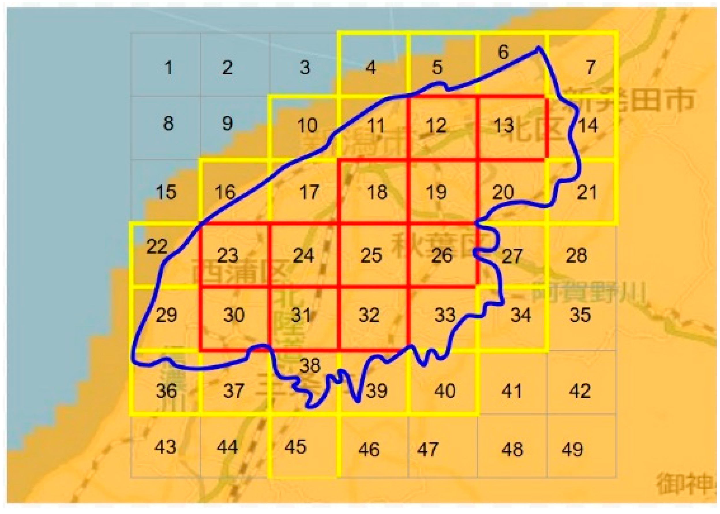
2.1. Mesh Design for PV Power Estimation

The CDF data highlighted in Figure 1, Figure 2, Figure 3 and Figure 4, with orange, gray, dark blue, clear green, and white colors, refer to sunny, cloudy, rainy, rainy and snowy, and snowy and cloudy conditions, respectively. The dates are 28 January, 13:00 p.m. in Figure 1; 14 May 2024, 13:00 p.m. in Figure 2; 22 July 2024, 13:00 p.m. in Figure 3; and 21 July 2024, 14:00 p.m. in Figure 4. In this paper, the mesh [40,41] corresponding to the CDF data has the topology of a network whose components are all directly connected to every other component. Also, it has a number of regular openings every linear inch or centimeter that are digitally drawn on Google Drawings, as shown in Figure 2, Figure 3 and Figure 4. The mesh covers the 726.45 km2 of Niigata City inhabited by 505,272 people in 2024 [42] and is placed onto the NHK CDF [40] data in Google Drawings. Figure 2, Figure 3 and Figure 4 show examples for winter, spring, summer, and autumn 2024 at 1 p.m. As mentioned in Section 1, the dataset for autumn is considered the same as that for spring in this paper as a setting. In our previous research [38], we did not set a land distribution ratio based on the CDF data like in this research, and even the proposed mesh method is different.
*
The picture is taken from the CDF data and Google Maps;
*
A mesh is designed on the picture to cover Niigata City.
The scale of the picture is 1:20 km both for the CDF data and Google Maps. Therefore, we were able to draw a blue line which represents Niigata City in Google Drawings, along with 7 × 7 rectangles that form a mesh with the red, yellow, and gray lines, as shown in Figure 1, Figure 2 and Figure 3. Each rectangle is identified by a number to complete the entire mesh, counting from 1 to 49. The rectangles completely inside the shape of Niigata City are indicated in red, while the others are yellow and gray.
To obtain the photovoltaic estimated power (PVE), each rectangle is set to have both a CDF and a land coverage percentage. Endorsed by the National Aeronautics and Space Administration (NASA) and the National Oceanic and Atmospheric Administration (NOAA), Table 1 delineates the association between the power generation and the configurations of the CDF [43,44], while, referring to Figure 4, Table 2 elaborates more about the PVE by clarifying the land coverage settings in detail. The entire mesh is formed of 49 rectangles represented in column 1 of Table 2, and each rectangle is identified by a number. Furthermore, in column 1, line 2 of Table 2, rectangles 1–3, 8, 9, 15, 28, 35, and 41–49 are, on referring to the blue line in Figure 4, not in Niigata City.
Concerning column 2 of Table 2, we set a land distribution ratio for each rectangle based on the CDF data. Assuming that the inside of the blue line representing the shape of Niigata City is full of land, we can, for further illustration purposes, set the land distribution value for rectangles 12, 13, 18, 19, 23–26, 31, and 32 to 1 each, which means they are full of land. But for rectangles 1–3, 8, 9, 15, 28, 35, and 41–49, there is no connection with the blue line, meaning that we can set their respective land distribution to 0, which means no land. Then, as the blue line covers parts of rectangles 4–7, 10–14, 16–27, 29–34, and 36–40, we can accordingly set their land distribution valued to 0, 0.17, 0.65, 0.08, 0.15, 0.7, 1, 1, 0.4, 0.4, 0.95, 1, 1, 0.8, 0.2, 0.4, 1, 1, 1, 1, 0.27, 0.75, 0.99, 1, 1, 0.8, 0.1, 0.21, 0.17, 0.56, 0.32, and 0.08, respectively. These values are fixed and not related to the daily weather, time, CDF, or season of the year. Equations (1) and (2) support the AC PV generation output by the inverter.
P t ( W ) = 90 100 × 93 × 10 6 × C S P 30 × 1 49 L C I 1 49 R L R
where Pt is the Alternating Current (AC) PV generation output by the inverter, and CSP, LCI, and RLR stand for the clear sky power, Land and Cloud Impact, and Related Land Ratio, respectively.
L C I = R L R × S A × 1 + C A × 0.3 + R A × 0.1
where SA, CA, and RA refer to the Sunny Cloud Amount, Cloudy Cloud Amount, and Rainy Cloud Amount in Table 1. The ratio of rainy with snow, as well as snowy cloudy conditions, is not considered in Equation (2) because, as shown in Table 1, the generation capacity is set to zero. Equation (2) is developed to calculate the corresponding land and cloud impact for every rectangle counted from 1 to 49. The results are presented in the third column of Table 2.
Equally, the clear sky data are collected over 24 h (00 a.m.–11 p.m.), and in column 4 of Table 2, we show the temporal clear sky power results. We used the Bird model, which is a model that estimates clear sky conditions based on the location settings (latitude, longitude, etc.). The clear sky days are assumed for a leap year [45], and for each day of the year, the Bird model provides (in W/m2) data about the direct beam, the direct horizontal irradiance, and the diffuse horizontal irradiance. Among these, the present research utilized the global horizontal irradiance, and it was assumed in the simulations that the maximum irradiance was achieved at the solar panel rated power, i.e., 30 Wp at 12 a.m., for the winter, spring, and summer cases, as we can see from the green curves in Figure 5, Figure 6 and Figure 7. The values presented in column 4 of Table 2 are for the 30 Wp solar panel at Niigata University but are converted into 93 MWp when plotting them. After conversion, we assume an inverter efficiency of 90% to obtain P t ( W ) . For 21 July 2024, we obtain P 2 P M M W = 39.1 , as shown in the last line of Table 2. The photovoltaic module type used at a laboratory level of Niigata University is 0.172 m2, Model: #893TGM500-24V72, for a 24-volt rechargeable battery and appliance.
Since we used the Bird model for the PV clear sky power estimations in Niigata City [38,45], Figure 5, Figure 6 and Figure 7 highlight in green the clear sky data for the 93 MWp PV power plant for the winter, spring, and summer cases, respectively. Then, from Equations (1) and (2), we compute the DC power in Excel., i.e., to obtain the PVE before the inverter, highlighted in red, and given in orange are the converted measured data from the 30 Wp solar panel at Niigata University.
Due to the influence of temperature on solar panels, the 30 Wp solar panel’s measured value may sometimes be higher than the rated value, which justifies why in Figure 6 the converted measured data are higher than the clear sky data at 8 and 9 a.m. The impact of this error is checked from the simulation results of the electricity frequency fluctuations.

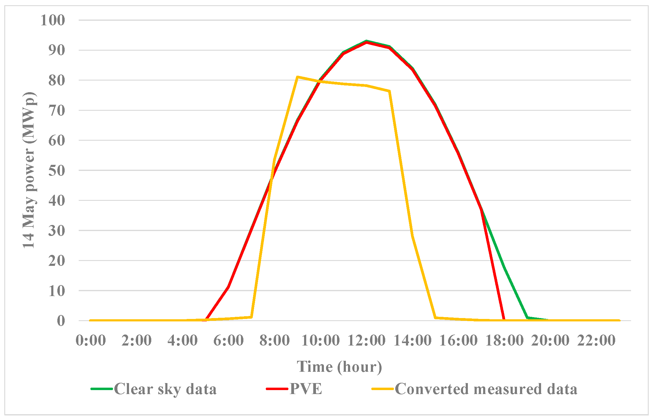
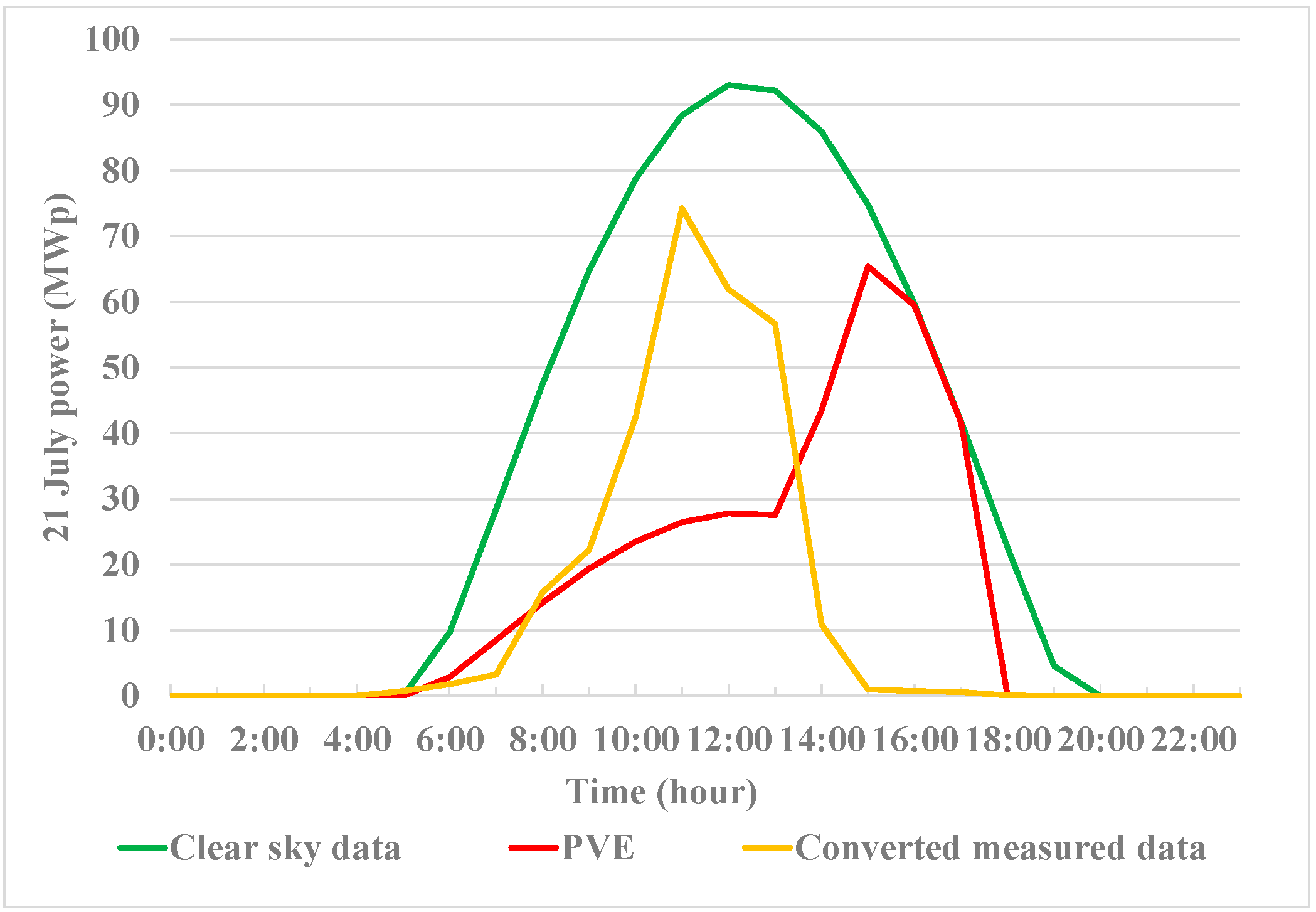
2.2. Daily Power Curve for Niigata City

Tohoku Electric Power Network Co., Inc. serves seven prefectures in Japan, including Niigata. Figure 8 presents an overview of the grid configurations and the locations of the power stations, as specified in the 2024 integrated report of the Tohoku Electric Power Group [34]. The daily power curve information can be found on the power company’s website, after which step the values are distributed to align with the population of Niigata City. The MATLAB interpolation table converts the daily power curve hourly data into 1 min data through spline interpolation.
Figure 9 shows the required power at Niigata City on 28 January, 13 May, and 17 July 2024 for winter, spring, and summer cases.

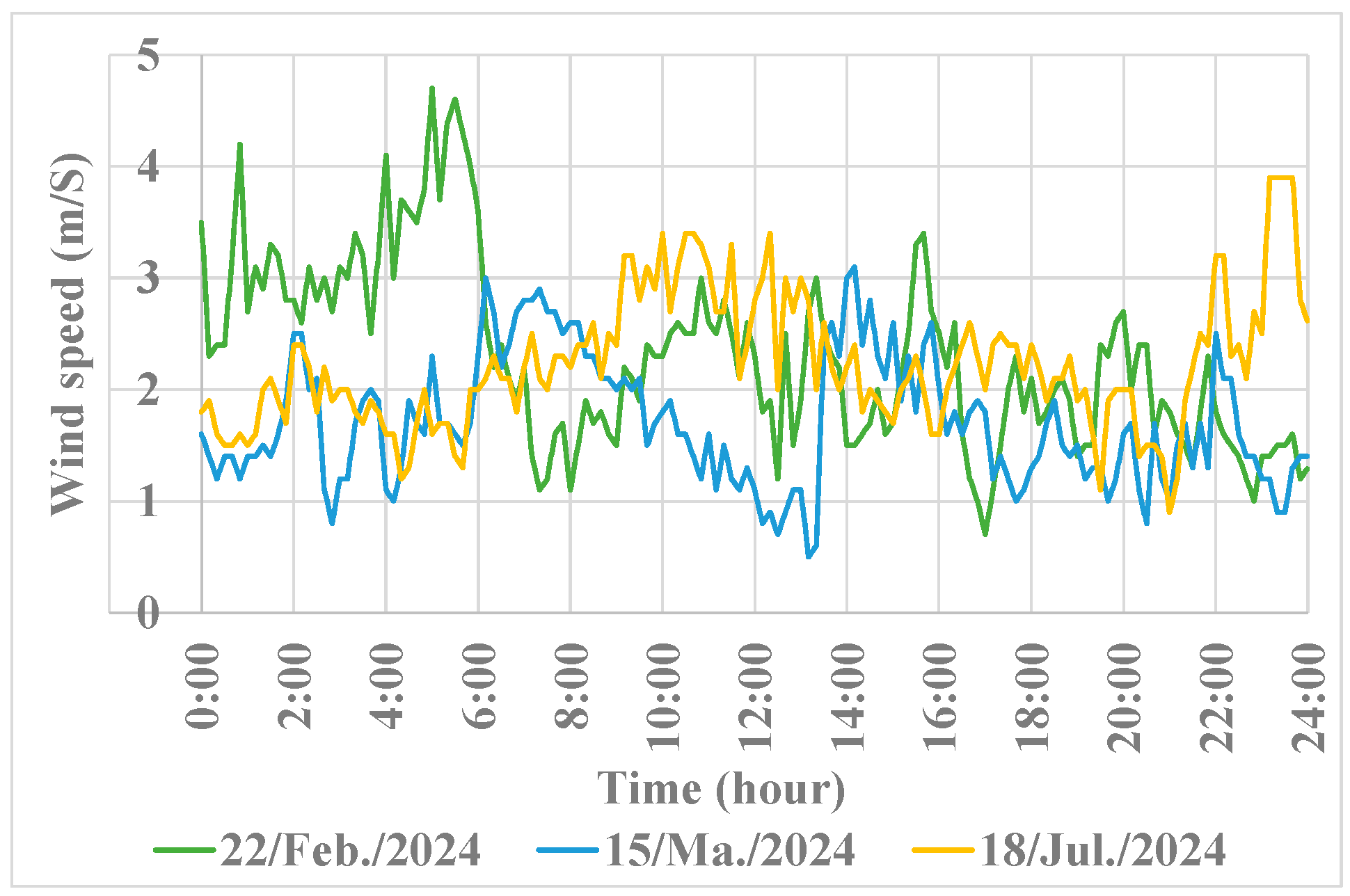
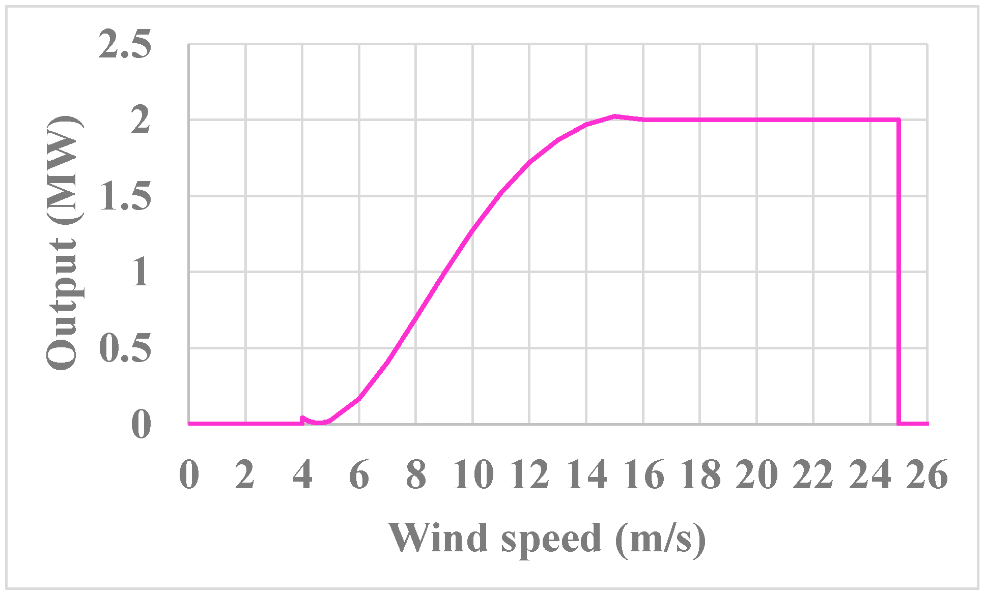
3. Prediction of the Wind Power

The start-up test results for a vertical-shaft, single-wheel, single-flow Francis turbine from Okumen Power Station (rated power = 34.5 MW), run under the jurisdiction of Niigata Enterprises Bureau and shown in Table 3 for reference purposes, indicate that the starting time of the hydroelectric generator is 347 s. From this, a cut-off time of 360 s or 6 min is set as the starting time of the hydro generator. That is, to prevent a lack of electricity generation, 6 min autoregressive wind speed prediction (6ARW) is required. A MATLAB interpolation table is used to convert the wind speed GPV hourly data and actual wind speed 10 min data into 1 min data through spline interpolation.
So, the wind power is predicted from the wind speed using 6ARW. The 1 h GPV wind farm (1HWF) is the planned power generation obtained from the GPV wind speed prediction data through Excel computation.
Due to the geographical wind distribution, the output of a wind farm with 10 turbines is not the same as the multiplied output of a single turbine. For example, Figure 10 highlights a wind farm arrangement with lines A and B. The first line includes turbines A1 to A5, which are vertical in the direction of wind and parallel to line B, consisting of turbines B1 to B5. For example, we assume that the wind observed in line A will reach line B after 2 min and that the distance between these 2 lines is 1 km. The distance between turbines A1 and A2 is 1 km, which is also the same for the distances between A2 and A3, A3 and A4, and A4 and A5, as well as between A1 and B1, B1 and B2, B2 and B3, B3 and B4, and B4 and B5, as shown in Figure 10. Furthermore, the power performance of the aerodynamics of a double-rotor vertical-axis wind turbine (VAWT) array is significantly influenced by the relative rotational direction and positioning, approximately 8% in the power coefficient (CP), while it is marginally dependent on the relative phase lag [46]. Nonetheless, consideration of the wind’s geographical distribution’s impact on the wind farm power calculations is acknowledged as one of the limitations of this study.
We set testing and evaluation days chosen randomly in all seasons to perform the simulations. The power system control in this research was established by using testing day data and evaluated using evaluation day data. So, the testing day and evaluation days in winter were 28 January and 22 and 24 February, respectively. In spring, the testing days were 13 and 15 May, while the evaluation days were 14 and 16 May. Then, in summer, 17 and 21 July were the testing days and 18 and 22 July the evaluation days. We set the wind farm capacity to 20 MW by combining 2 MW Vestas wind turbines [47].
Since wind speed is predicted using the autoregressive (AR) model, a brief introduction to this model may be required. An AR model is a time series model that predicts the current value of a variable using its historical values. It serves as one of the fundamental tools for making more accurate and data-informed decisions [48]. An AR model, often referred to as a conditional model, Markov model, or transition model, can be expressed as AR (j), in which specific lagged values of Wt serve as the predictor variables. Lags refer to situations where the outcomes from a particular period influence those of subsequent periods. The variable j is referred to as the order. For instance, when j equals 1, it represents the first-order autoregressive process, indicated by AR (1). The outcome variable in this case is linked only to values from one time period earlier, specifically the value at (t − 1). An AR process of the second or third order would refer to data from two or three time periods earlier, respectively. AR (j) is expressed in Equation (3) [49].
W t = δ + φ 1 W t 1 + φ 2 W t 2 + + φ j W t 1 + A t
where
W t 1 ,   W t 2 ,     W t j ,   a r e   t h e   l a g s A t   i s   t h e   r a n d o m n e s s w i t h   μ   t h e   p r o c e s s   m e a n ,   δ = 1 i = 1 j β i μ
Figure 11 shows the actual wind speed in Niigata City on 22 February, 15 May, and 18 July 2024.
The JMA provides wind speed data at sea level, and Niigata City is located at a height of 15.1 m [50]. We need to bring actual and GPV wind speed prediction data for both the site and Vestas’s wind turbine specifications. We call this wind speed correction in this research following Hellmann’s exponential formula, defined in Equation (4) [51], and to perform this correction, Table 4 [52] provides the required coefficients. From Niigata City’s topography, we divide the ratio of the speed at sea in the vicinity by that on the coast in windward locations to obtain the required wind speed ratio for computing the correction. Figure 12, Figure 13 and Figure 14 show the related wind speed predictions, together with the GPV wind speed results for the 3 seasons of the year 2024, as examples. The GPV-corrected wind speed used to calculate the planned power generation is represented in green, while the actual corrected wind speed is represented in red.
v v 0 = H H 0 α
where v represents the speed corresponding to the height H , while v 0 denotes the speed associated with the height H 0 . The coefficient α, known as the friction coefficient or Hellman’s exponent, varies based on the topography of a specific location. In this research, it is commonly assumed to be a value of 1/7.
Since the power system control in this research was established using testing day data and evaluated using evaluation day data, chosen randomly, simulations were made for many different days in the same season and were also chosen randomly for presentation in this paper, which explains why the dates in the figures are sometimes different for the same season of the year.
The wind turbine power curve is highlighted in Figure 15. In fact, by choosing a couple of points (power, wind speed) from the technical datasheet on the Vestas V80-2.0 MW wind turbine (Vestas Wind Systems A/S, Randers, Denmark), we set the polynomial order to 5 in Excel, and using the Excel LINEST function, we obtained −10.2, +836.3, −25,696.7, +352,324.2, −1,909,204.4, and 3,481,877.4, respectively, as the equation’s coefficients. By substituting the variable in this polynomial equation with wind speeds ranging from 0 to 25 m/s and using Excel’s “IF function” with conditions based on the cut-in (4 m/s), rated (16 m/s), and cut-out (25 m/s) wind speeds defined on the datasheet, we were able to derive the results presented in Figure 15.

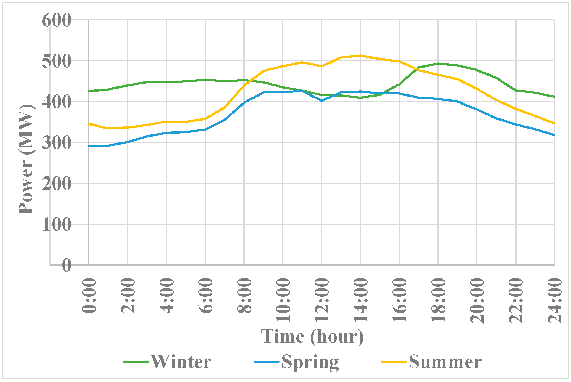
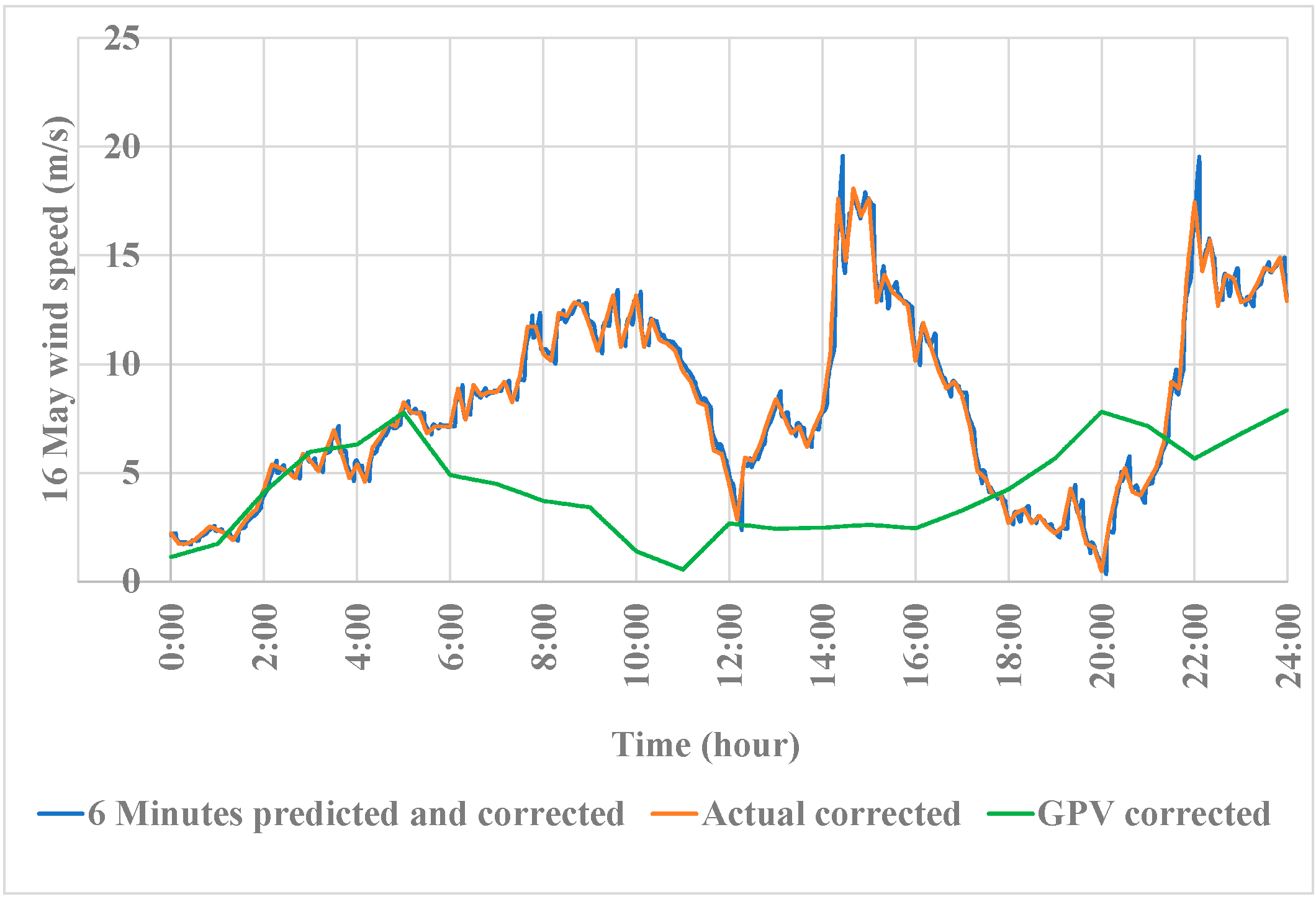
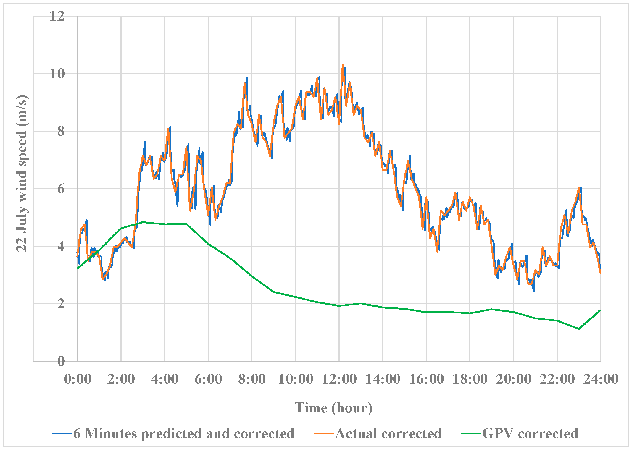
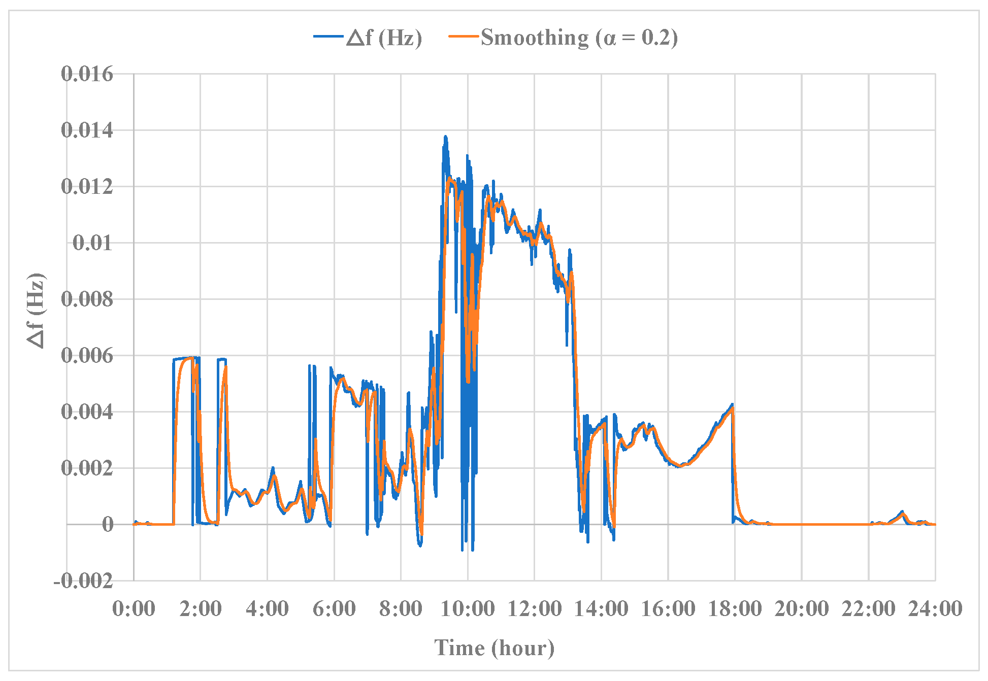
4. Power Balance Simulation

Hydro power is added up to 20 MW to obtain ΔP = 0. When a hydro power generator is in operation, variable output control with an assumed rate of 10%/min is performed [53]. In the case of a shutdown state, it takes 6 min to start up, so wind speed predictions are required after 6 min, and the system is controlled to eliminate the difference from the daily power curve. We can only increase hydro at a maximum rate of 10%/min. Figure 16 elaborates more about the power balance. In fact, solar and wind are intermittent sources compared to hydro, i.e., the necessity of using hydro power, as described in Figure 16, is very important in this research.
In Figure 16, AR6 refers to the 6 min autoregressive wind farm prediction, like 6ARP; Plan refers to the 1HWF, like 1HP; and Actual refers to the wind farm’s actual power (WFA), like the PVE.

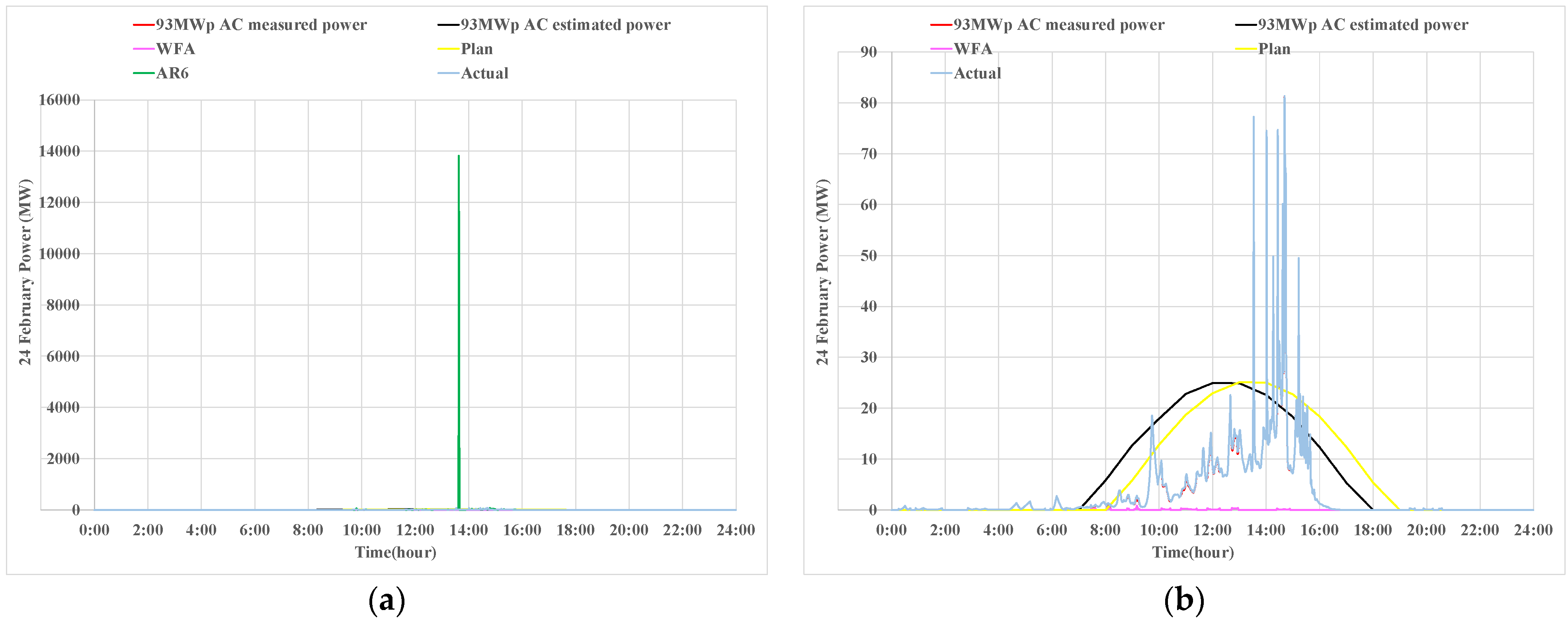
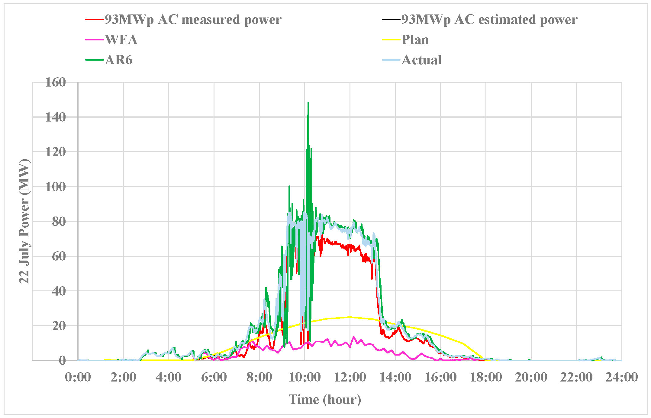
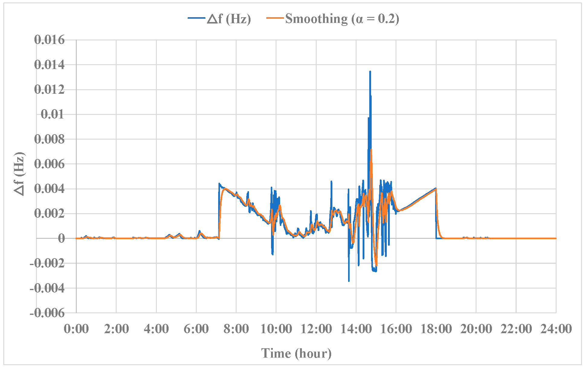
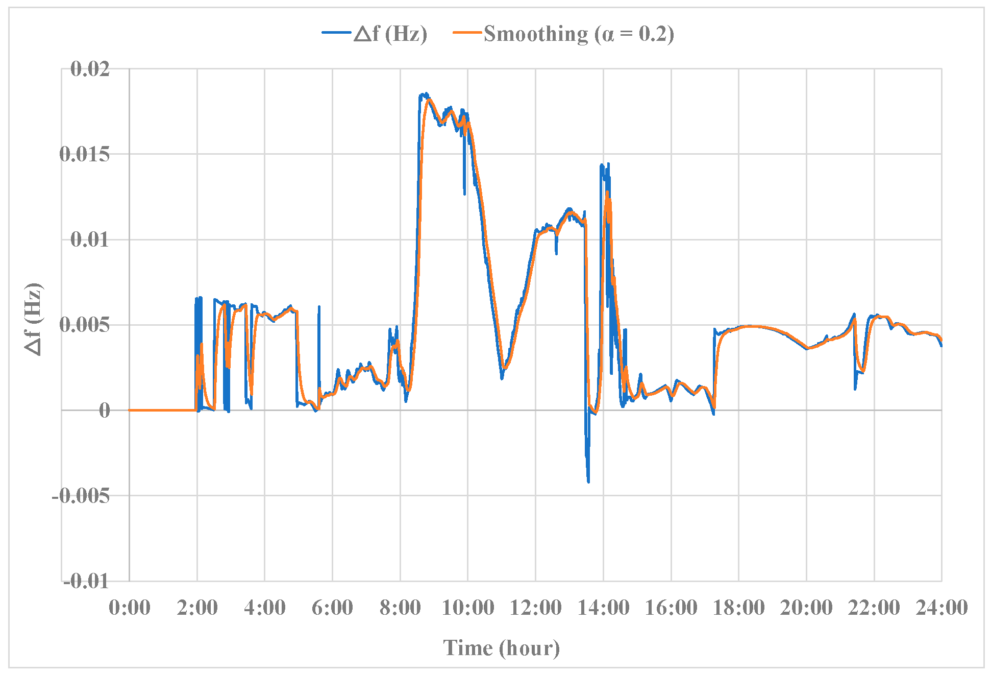
4.1. Simulation Results

From these wind speeds, we can simulate the power generation curves, as shown in Figure 17, Figure 18 and Figure 19.
The 6ARP from Python unexpectedly gave 13,814 MW at 13:38 p.m. in Figure 17a, which is very high compared to the other power curve values, preventing them from fully being seen. This error might have been related to Python’s autoregressive (AR) model simulation, and its influence on the frequency stability results is discussed in a later section. However, by isolating AR6 in Figure 17a, we can obtain Figure 17b, showing the other power curves in detail.
Equation (5) supports the frequency fluctuations in the electricity calculation. We set a curve smoothing factor of 0.2 in Excel. So, the frequency fluctuation f   ( H z ) at the power grid is
f = P P K
where P   ( M W ) represents all of the generated output power, the same as the daily power curve, and P ( M W ) the difference between the predicted photovoltaic and wind farm outputs. Then, K   ( % M W / H z ) represents the frequency characteristic. Considering the worst-case scenario, we use a K value of 10 in this research. Figure 20, Figure 21 and Figure 22 highlight the change in the frequency of electricity accordingly.

4.2. Discussions

The PSS of the proposed HPP is evaluated from the FS simulation results. Tohoku Electric Power Network Co., Inc. provides electricity at 101 V–50/60 Hz, with permissible limits of ±6 Volts and ±0.2 Hz for the voltage and frequency fluctuations, respectively; i.e., if the proposed HPP’s simulation results for the fluctuations in electricity frequency for the testing and evaluation days are within ±0.2 Hz, PSS is achieved. The proposed HPP features a 93 MWp PV power plant located in Niigata City, complemented by a thermal power facility operated by Tohoku Electric Power Network Co., Inc., which adheres to the daily power generation curve. Furthermore, it includes a 20 MW WP plant, which is supported by a 20 MW hydropower plant. After the seasonal simulations, we reach a maximum value of +0.013 Hz at 2:42 p.m. and a minimum value of −0.003 Hz at 1:38 p.m. in winter and then a maximum value of +0.018 Hz at 08:46 a.m. and a minimum value of −0.004 Hz at 1:34 p.m in spring. In summer, we obtain −0.00092 Hz at 10:09 a.m. as the minimum value and +0.0138 Hz at 09:20 a.m. for the maximum value, which are all within ±0.2 Hz of the permissible limits of Tohoku Electric Power Network Co., Inc. and confirm the proposed system’s integration into the grid. Despite the error in Figure 17a, the FS results are excellent.

5. Conclusions

After optimization of the PV component of the proposed HPP, PVs were combined with thermal, wind, and hydro power to perform the simulations. As a result, the PSS was evaluated from the simulation results of the fluctuations in the frequency of electricity within the permissible range of the local power operator in Niigata City. So, electricity is supplied stably and optimally to residents, preventing them from experiencing flickering lights, unexpected blackouts, and soaring electricity bills caused by extreme weather conditions and aging power infrastructure. The proposed HPP is a good investment for grid infrastructure modernization. The proposed mesh method can be implemented in any HPP in the world that has solar power generation as part of its components to improve on the energy efficiency of the PV output power. By providing electricity that leads to a comfortable life and safety in the context of climate change, many health issues and accidents caused by an unstable and aging power grid can be avoided in society. The HPP’s grid integration in Niigata City could contribute to increased decarbonization of the power generation sector. In addition to [28], hydropower has significantly contributed to the power balance here. Renewable energy has successfully shown its relevance to PSS. As some countries are making efforts to reduce the effects of global warming, this research is clearly within this trend towards a sustainable planet. However, some limitations remain. First, a numerical model including optimization of the mesh size could be considered in future work to improve upon the proposed PV output power results. And then, this numerical model would considerably reduce the time to estimate the required coefficients of the SA, CA, and RA for calculating the LCI. Secondly, the influence of the geographical wind distribution on the wind farm power output could be addressed in future research. Then, the quantity of CO2 emissions avoided by implementing the proposed HPP could also be investigated in future work.

Author Contributions

Conceptualization: T.D.T.M. and A.S. Methodology: T.D.T.M. and A.S. Software: T.D.T.M. and Y.L. Validation: T.D.T.M., A.S., Y.B. and Y.L. Formal analysis: A.S., T.D.T.M., Y.L. and Y.B. Investigation: T.D.T.M., A.S., Y.B. and Y.L. Resources: T.D.T.M., Y.L. and Y.B. Data curation: T.D.T.M., Y.L. and Y.B. Writing—original draft preparation: T.D.T.M. Writing—review and editing: T.D.T.M., A.S. and Y.B. Visualization: T.D.T.M. and A.S. Supervision: A.S. Project administration: A.S. Funding acquisition: A.S. All authors have read and agreed to the published version of the manuscript.

Funding

This research received no external funding.

Data Availability Statement

The original contributions presented in this study are included in the article; further inquiries can be directed to the corresponding author.

Acknowledgments

The authors are grateful to the Renewable Energy Laboratory of the Faculty of Engineering of Niigata University for providing the laboratory facilities.

Conflicts of Interest

The authors declare no conflicts of interest.

Nomenclature

PVSolar photovoltaic
HCHydropower capacity
6ARWSix-minute autoregressive wind speed prediction
6ARPSix-minute autoregressive PV power prediction
1HWFOne-hour GPV wind farm
1HPOne-hour NHK prediction
WFAWind farm actual power
PVEPhotovoltaic estimated power
PSSPower system stability
FSFrequency stability
HPPHybrid power plant
JMAJapan Meteorological Agency
CDFNHK cloud distribution forecast
SDGSustainable development goal
WPWind power
GPVGrid Point Value
NHKJapan Broadcasting Corporation
DERsDistributed energy resources
COPConference of the parties
UNUnited Nations
VREVariable renewable energy

References

  1. Westbrook, K. The Power Grid Crisis: What It Means for Everyday Families. Climate Science. Available online: https://climatecosmos.com/climate-science/the-power-grid-crisis-what-it-means-for-everyday-families/ (accessed on 19 February 2025).
  2. Saleh, A.M.; István, V.; Khan, M.A.; Waseem, M.; Ahmed, A.N.A. Power system stability in the Era of energy Transition: Importance, Opportunities, Challenges, and future directions. Energy Convers. Manag. X 2024, 24, 100820. [Google Scholar] [CrossRef]
  3. Hassan, Q.; Algburi, S.; Sameen, A.Z.; Salman, H.M.; Jaszczur, M. A review of hybrid renewable energy systems: Solar and wind-powered solutions: Challenges, opportunities, and policy implications. Results Eng. 2023, 20, 101621. [Google Scholar] [CrossRef]
  4. Bhattacharyya, A.; Yoon, S.; Hastak, M. Economic Impact Assessment of Severe Weather–Induced Power Outages in the US. J. Infrastruct. Syst. 2021, 27, 04021038. [Google Scholar] [CrossRef]
  5. Hansen, A.D.; Adamou, P.; Giagkou, X.; Rigas, F.; Sakamuri, J.; Altin, M.; Nuno, E.; Sørensen, P. Dynamic Modeling of Wind-Solar-Storage Based Hybrid Power Plant. In Proceedings of the 18th Wind Integration Workshop, Dublin, Ireland, 16–18 October 2019; Available online: https://backend.orbit.dtu.dk/ws/portalfiles/portal/197791357/9B_1_WIW19_248_paper_Das_Kaushik.pdf (accessed on 17 March 2025).
  6. International Energy Agency. The Power of Transformation: Wind, Sun and the Economics of Flexible Power Systems. IEA 2014, 10, 160–179. Available online: https://iea.blob.core.windows.net/assets/b6a02e69-35c6-4367-b342-2acf14fc9b77/The_power_of_Transformation.pdf (accessed on 27 December 2024).
  7. Chayapathi, V.; Sharath, B.; Anitha, G.S. Voltage Collapse Mitigation By Reactive Power Compensation At the Load Side. Int. J. Res. Eng. Technol. 2013, 2, 251–257. [Google Scholar] [CrossRef]
  8. Sattar, F.; Ghosh, S.; Isbeih, Y.J.; El Moursi, M.S.; Al Durra, A.; El Fouly, T.H.M. A predictive tool for power system operators to ensure frequency stability for power grids with renewable energy integration. Appl. Energy 2024, 353, 122226. [Google Scholar] [CrossRef]
  9. Hatziargyriou, N.; Milanovic, J.; Rahmann, C.; Ajjarapu, V.; Canizares, C.; Erlich, I.; Hill, D.; Hiskens, I.; Kamwa, I.; Pal, B.; et al. Definition and Classification of Power System Stability-Revisited & Extended. IEEE Trans. Power Syst. 2021, 36, 3271–3281. [Google Scholar] [CrossRef]
  10. Shair, J.; Li, H.; Hu, J.; Xie, X. Power system stability issues, classifications and research prospects in the context of high-penetration of renewables and power electronics. Renew. Sustain. Energy Rev. 2021, 145, 111111. [Google Scholar] [CrossRef]
  11. Chandarahasan, C.; Percis, E.S. The accessible large-scale renewable energy potential and its projected influence on Tamil Nadu’s grid stability. Indones. J. Electr. Eng. Comput. Sci. 2023, 31, 609–616. [Google Scholar] [CrossRef]
  12. Qin, B.; Wang, M.; Zhang, G.; Zhang, Z. Impact of renewable energy penetration rate on power system frequency stability. Energy Rep. 2022, 8, 997–1003. [Google Scholar] [CrossRef]
  13. Rahman, A.; Murad, S.W.; Mohsin, A.K.M.; Wang, X. Does renewable energy proactively contribute to mitigating carbon emissions in major fossil fuels consuming countries? J. Clean. Prod. 2024, 452, 142113. [Google Scholar] [CrossRef]
  14. Yuping, S.; Shenghu, S.; Tiwari, A.K.; Khan, S.; Zhao, X. Impacts of renewable energy on climate risk: A global perspective for energy transition in a climate adaptation framework. Appl. Energy 2024, 362, 122994. [Google Scholar] [CrossRef]
  15. HivePower. Grid Stability Issues with Renewable Energy Sources: How They Can Be Solved. 22 March 2021. Available online: https://www.hivepower.tech/blog/grid-stability-issues-with-renewable-energy-how-they-can-be-solved (accessed on 6 December 2024).
  16. International Energy Agency. Net Zero by 2050 a Roadmap for the Global Energy Sector. Available online: https://iea.blob.core.windows.net/assets/deebef5d-0c34-4539-9d0c-10b13d840027/NetZeroby2050-ARoadmapfortheGlobalEnergySector_CORR.pdf (accessed on 15 November 2024).
  17. Arbabzadeh, M.; Sioshansi, R.; Johnson, J.X.; Keoleian, G.A. The role of energy storage in deep decarbonization of electricity production. Nat. Commun. 2019, 10, 3413. [Google Scholar] [CrossRef]
  18. Wei, H.; Xin, L.; Liu, P. Types of CO2 Emission Reduction Technologies and Future Development Trends. Eng. Rural Dev. 2022, 25, 50–54. [Google Scholar] [CrossRef]
  19. Kosugi, T.; Tokimatsu, K.; Yoshida, H. Evaluating new CO2 reduction technologies in Japan up to 2030. Technol. Forecast. Soc. Change 2005, 72, 779–797. [Google Scholar] [CrossRef]
  20. KIZUNA. Climate Transition Bonds Show Japan’s Commitment to Carbon Neutrality. 27 September 2024. Available online: https://www.japan.go.jp/kizuna/2024/09/climate_transition_bonds.html (accessed on 12 December 2024).
  21. Tohoku Electric Power Group. Tohoku Electric Power Group Sustainability Report 2023; Tohoku Electric Power Group: Sendai City, Japan, 2023; Available online: https://www.tohoku-epco.co.jp/ir/report/integrated_report/pdf/tohoku_sustainability2023en.pdf#page=15 (accessed on 29 December 2024).
  22. Tohoku Electric Power Network Co. Feed-in Tariff Scheme for Renewable Energy. Available online: https://nw.tohoku-epco.co.jp/consignment/renew/pdf/saisei.pdf (accessed on 26 December 2024). (In Japanese).
  23. Grant, E.; Clark, C.E. Hybrid power plants: An effective way ofdecreasing loss-of-load expectation. Energy 2024, 307, 132245. [Google Scholar] [CrossRef]
  24. Kim, J.; Millstein, J.H.; Wiser, D.; Mulvaney-Kemp, R. Renewable-battery hybrid power plants in congested electricity markets: Implications for plant configuration. Renew. Energy 2024, 232, 121070. [Google Scholar] [CrossRef]
  25. Denholm, P.; Nunemaker, J.; Gagnon, P.; Cole, W. The potential for battery energy storage to provide peaking capacity in the United States. Renew. Energy 2020, 151, 1269–1277. [Google Scholar]
  26. Denholm, P.; Mai, T. Timescales of energy storage needed for reducing renewable energy curtailment. Renew. Energy 2019, 130, 388–399. [Google Scholar] [CrossRef]
  27. Aziz, A.; Oo, A.T.; Stojcevski, A. Analysis of frequency sensitive wind plant penetration effect on load frequency control of hybrid power system. Electr. Power Energy Syst. 2018, 99, 603–617. [Google Scholar] [CrossRef]
  28. Ji, W.; Hong, F.; Zhao, Y.; Liang, L.; Du, H.; Hao, J.; Fang, F.; Liu, J. Applications of flywheel energy storage system on load frequency regulation combined with various power generations: A review. Renew. Energy 2024, 223, 119975. [Google Scholar] [CrossRef]
  29. Kennedy, C.; Bertram, D.; White, C.J. Reviewing the UK’s exploited hydropower resource (onshore and offshore). Renew. Sustain. Energy Rev. 2024, 189, 113966. [Google Scholar] [CrossRef]
  30. Sample, J.E.; Duncan, N.; Ferguson, M.; Cooksley, S. Scotland’s hydropower: Current capacity, future potential and the possible impacts of climate change. Renew. Sustain. Energy Rev. 2015, 52, 111–122. [Google Scholar] [CrossRef]
  31. Sarmiento-Vintimilla, J.C.; Larruskain, D.M.; Torres, E.; Abarrategi, O. Assessment of the operational flexibility of virtual power plants to facilitate the integration of distributed energy resources and decision-making under uncertainty. Int. J. Electr. Power Energy Syst. 2024, 155, 109611. [Google Scholar] [CrossRef]
  32. Karapici, V.; Trojer, A.; Lazarevikj, M.; Pluskal, T.; Chernobrova, A.; Nezirić, E.; Zuecco, G.; Alerci, A.L.; Seydoux, M.; Doujak, E.; et al. Opportunities of hidden hydropower technologies towards the energy transition. Energy Rep. 2024, 12, 5633–5647. [Google Scholar] [CrossRef]
  33. Zhou, C.; Doroodchi, E.; Moghtaderi, B. Figure of Merit Analysis of a Hybrid Solar-Geothermal Power Plant. Engineering 2013, 5, 26. [Google Scholar] [CrossRef]
  34. Tohoku Electric Power Group. Tohoku Electric Power Group Integrated Report 2024. 2024. Available online: https://www.tohoku-epco.co.jp/ir/report/integrated_report/pdf/tohoku_integratedreport2024en.pdf (accessed on 29 December 2024).
  35. Ahsan, L.; Iqbal, M. Dynamic Modeling of an Optimal Hybrid Power System for a Captive Power Plant in Pakistan. Jordan J. Electr. Eng. 2022, 8, 195. [Google Scholar] [CrossRef]
  36. Testbook Edu Solutions Pvt. Ltd. Power System Stability: Know Definition & Types Of Stability. Testbook. Available online: https://testbook.com/electrical-engineering/power-system-stability (accessed on 19 February 2025).
  37. Energiewende, A. Integrating Renewables into the Japanese Power Grid by 2030. 148/1-S-2019/EN. Available online: https://www.renewable-ei.org/pdfdownload/activities/REI_Agora_Japan_grid_study_FullReport_EN_WEB.pdf (accessed on 30 January 2025).
  38. Tchokomani Moukam, T.D.; Sugawara, A.; Shawapala, I.L.; Bello, Y.; Li, Y. Stabilization of Electricity by Mesh Method and Combination of Renewable Energy System. In Proceedings of the International Council on Electrical Engineering Conference 2024, Kitakyushu, Japan, 30 June–4 July 2024. [Google Scholar]
  39. JMA/GPV Weather Maps. 2024. Available online: https://www.basso-continuo.com/WeatherGPV/index_e.htm (accessed on 30 December 2024).
  40. NHK (Japan Broadcasting Corporation). NHK News Web. 2024. Available online: https://www.nhk.or.jp/kishou-saigai/city/status/15100001510700/ (accessed on 30 December 2024).
  41. Vocabulary.com. Mesh. 2024. Available online: https://www.vocabulary.com/dictionary/mesh (accessed on 30 December 2024).
  42. Population of Cities in Japan 2024. 2024. Available online: https://worldpopulationreview.com/cities/japan (accessed on 25 October 2024).
  43. Introduction to Clouds. Available online: https://www.ncei.noaa.gov/sites/default/files/sky-watcher-cloud-chart-noaa-nasa-english-version.pdf (accessed on 9 February 2024).
  44. Zhu, X.; Yan, J.; Lu, N. A Graphical Performance-Based Energy Storage Capacity Sizing Method for High Solar Penetration Residential Feeders. IEEE Trans. Smart Grid 2017, 8, 3–12. [Google Scholar] [CrossRef]
  45. Brownson, T.P.S.U.J.; Earth, C.O.; Sciences, M. Clear Sky Model and Measured Irradiance Data. 2023. Available online: https://www.e-education.psu.edu/eme810/node/698 (accessed on 20 March 2024).
  46. Sahebzadeh, S.; Rezaeiha, A.; Montazeri, H. Vertical-axis wind-turbine farm design: Impact ofrotor setting and relative arrangement on aerodynamic performance ofdouble rotor arrays. Energy Rep. 2022, 8, 5793–5819. [Google Scholar] [CrossRef]
  47. Vestas. VestasV80-2.0 MWFacts and Figures. 2011. Available online: https://www.ledsjovind.se/tolvmanstegen/Vestas%20V90-2MW.pdf (accessed on 19 February 2024).
  48. Chaudhari, J. Understanding Autoregressive (AR) Models for Time Series Forecasting. 25 July 2023. Available online: https://jaichaudhari.medium.com/understanding-autoregressive-ar-models-for-time-series-forecasting-508016498a1e (accessed on 31 December 2024).
  49. 2025 Statistics How To. Autoregressive Model: Definition & The AR Process. Statistics How To. 2025. Available online: https://www.statisticshowto.com/autoregressive-model/ (accessed on 19 February 2025).
  50. J. M. Agency. JMA Height for Niigata. 2024. Available online: https://www.jma-net.go.jp/niigata/gaikyo/geppo/kishou_ichiran.pdf (accessed on 17 March 2025). (In Japanese)
  51. Bañuelos-Ruedas, F.; Camacho, C.Á.; Rios-Marcuello, S. Methodologies Used in the Extrapolation of Wind Speed Data at Different Heights and Its Impact in the Wind Energy Resource Assessment in a Region. Wind. Farm-Tech. Regul. Potential Estim. Siting Assess. 2011, 97, 114. [Google Scholar] [CrossRef]
  52. Hiroshi, A.; Yasutsugu, K.; Meng, I. A method for estimating offshore winds using a three-dimensional wind model. Jpn. Soc. Civ. Eng. 2007, 54, 134. Available online: http://library.jsce.or.jp/jsce/open/00008/2007/54-0131.pdf (accessed on 13 October 2023). (In Japanese).
  53. Glattfelder, A.H.; Huser, L.; Dörfler, P.; Steinbach, J. Automatic Control for Hydroelectric Power Plants. In Control Systems, Robotics, and Automation; Encyclopedia of Life Support Systems (EOLSS): Oxford, UK, 2009; Volume XVIII, Available online: https://www.eolss.net/Sample-Chapters/C18/E6-43-33-04.pdf (accessed on 25 October 2023).
Figure 1. Mesh on CDF data (28 January 2024).
Energies 18 01540 g001
Figure 2. Mesh on CDF data (14 May 2024).
Energies 18 01540 g002
Figure 3. Mesh on CDF data (22 July 2024).
Energies 18 01540 g003
Figure 4. Mesh on CDF data (21 July 2024).
Energies 18 01540 g004
Figure 5. Power of the 93 MWp PV plant (24 February 2024).
Energies 18 01540 g005
Figure 6. Power of the 93 MWp PV plant (14 May 2024).
Energies 18 01540 g006
Figure 7. Power of the 93 MWp PV plant (21 July 2024).
Energies 18 01540 g007
Figure 8. Grid specifications and power station locations [34,37].
Energies 18 01540 g008
Figure 9. Daily power curves.
Energies 18 01540 g009
Figure 10. Example arrangement of the wind farm.
Energies 18 01540 g010
Figure 11. Actual wind speeds.
Energies 18 01540 g011
Figure 12. Wind speed forecasts (24 February 2024).
Energies 18 01540 g012
Figure 13. Wind speed forecasts (16 May 2024).
Energies 18 01540 g013
Figure 14. Wind speed forecasts (22 July 2024).
Energies 18 01540 g014
Figure 15. Wind turbine power curve [47].
Energies 18 01540 g015
Figure 16. Power balance flow chart.
Energies 18 01540 g016
Figure 17. Power generation change example (24 February 2024). (a) Error, (b) Without AR6.
Energies 18 01540 g017
Figure 18. Power generation change example (16 May 2024).
Energies 18 01540 g018
Figure 19. Power generation change example (22 July 2024).
Energies 18 01540 g019
Figure 20. Frequency fluctuation example (24 February 2024).
Energies 18 01540 g020
Figure 21. Frequency fluctuation example (16 May 2024).
Energies 18 01540 g021
Figure 22. Frequency fluctuation example (22 July 2024).
Energies 18 01540 g022
Table 1. Settings on clouds and power.
Coverage TypeAmountGenerating Power
Sunny01
Cloudy0.70.3
Rainy0.90.1
Rainy with snow10
Snowy10
Table 2. Power estimation method.
Rectangles (1–49)Related Land RatioLand and Cloud ImpactTemporal Clear Sky Power (Wp)
1–3, 8, 9, 15, 28, 35, 41–49000
4000
50.170.045390
60.650.1950
70.080.0240
100.150.078750
110.70.213.139
1210.39.202
1310.315.327
140.40.1220.884
160.40.425.402
170.950.617528.521
1810.330
1910.329.7254
200.80.2427.72
210.20.0624.132
220.40.3419.25
231113.46
2410.657.273
2510.31.463
2610.30
270.270.0810
290.750.750
300.990.990
3110.65
3210.3
330.80.24
340.10.03
360.210.21
370.170.17
380.560.364
390.320.096
400.080.024
P 2 P M M W 39.1
Table 3. Starting characteristics of hydro generators.
Time Since Start-Up Operation (s)
To the end of the bypass valve opening21
Until the end of the main valve opening156
Waterwheel start-up160
Up to excitation206
Until the automatic synchronization system is activated233
Up to synchronous parallelism245
Up to a given load347
Table 4. Carruthers wind speed ratios [52].
LocationRatio
At sea0.60
On a low-lying island0.55
Coast on the windward side, low land in the vicinity0.50
The downwind side of the coast, low land, or at sea in the vicinity0.40
Open land with few obstructions0.40
Shielded land and cities0.30
Disclaimer/Publisher’s Note: The statements, opinions and data contained in all publications are solely those of the individual author(s) and contributor(s) and not of MDPI and/or the editor(s). MDPI and/or the editor(s) disclaim responsibility for any injury to people or property resulting from any ideas, methods, instructions or products referred to in the content.

