Speed Estimation Method of Active Magnetic Bearings Magnetic Levitation Motor Based on Adaptive Sliding Mode Observer

Abstract

The installation distance between the speed sensor of the traditional rolling or sliding bearing permanent magnet synchronous motor and the rotor was very close, and the rotor of the magnetic levitation motor supported by Active Magnetic Bearings (AMBs) was in suspension. When the motor was running at high speed, the radial trajectory of the rotor changed all the time. The same frequency vibration caused by the unbalanced mass of the rotor made it easy to cause mechanical collision between the sensor and the rotor, resulting in direct damage of the sensor. Therefore, the sensorless speed estimation method was needed for the rotor control system of the magnetic levitation motor (MLM) to achieve high performance closed-loop control of speed and position. More importantly, in order to control or compensate the unbalanced force of the electromagnetic bearing rotor system, the rotor rotation speed signal should be obtained as accurately as possible. Therefore, the principle of adaptive sliding mode observer (SMO) was analyzed in detail by taking the rotor system of MLM as an example. Then, the sliding mode surface was designed, the speed estimation algorithm based on adaptive SMO was derived, and the stability analysis was completed. Finally, in order to verify the anti-disturbance performance of the system and the static and dynamic tracking performance of the motor, the dynamic performance was verified by increasing and decreasing the speed and load. The results showed that the speed estimation method based on adaptive SMO could achieve accurate speed estimation and had good static and dynamic performance.

1. Introduction

Active magnetic bearings (AMBs) have the advantages of non-friction, they are suitable for high-speed operation, and have a long service life [1]. The high-speed motor with active magnetic bearing has the advantages of small size and high-power density. Thus, AMB is widely used in the field of high-speed rotating machinery such as turbine sub-pump, compressor, flywheel energy storage, and so on [2].

During the operation of a maglev high-speed motor, the rotor is in a suspended state, and the centrifugal force generated by the rotor imbalance will cause rotor imbalance vibration [3,4,5]. In the study of unbalanced compensation strategy, Saeed [6] used a needle to control the vibration of a six-pole active magnetic bearing rotor system, the Cartesian control method, and a radial control method designed, respectively, and the robustness and vibration suppression effect of these two control methods are compared. In recent years, considering that tracking filters have the advantages of fast dynamic response, high tracking accuracy, and easy design, they have been studied in depth and applied in the unbalance compensation strategy.

Wu [7] introduced the Least-Mean-Square (LMS) algorithm into the PID control and proposed an unbalanced vibration control strategy based on the real-time filtering compensation of the rotor displacement signal. The vibration was eliminated by filtering the synchronous frequency and harmonic signals of the PID control input. Li [8] proposed an unbalanced compensation method based on the transformation of the Hypothetical Reference Frame (HRF) and analyzed the stability of the closed-loop system with compensation based on the theory of complex coefficients. Le [9] designed and optimized a radial magnetic bearing with a structure of separated control and bias coils to reduce the compensation current used for balancing the Unbalanced Magnetic Pull (UMP). Gong [10] proposed a four-factor variable polarity control method to suppress the coefficient of unbalance vibration, which requires multiple polarity switches to suppress the coefficient of unbalance vibration before and after the two rigid body modes.

Yao [11] proposed a linear active disturbance rejection control method based on model compensation and designed a linear extended state observer and a linear feedback control law with known model perturbation information, which can significantly reduce the rotor displacement and torque ripple. Li [12] proposed a current harmonic and unbalance suppression strategy based on the vector space decomposition control of Adaptive Linear Neuron (ALN), which can effectively suppress current harmonics and unbalances. In addition, Zhou [13] used the feature structure configuration method to directly establish the connection between the parameters of the feedback controller and the feature structure of the closed-loop system to realize the active control of electromagnetic bearing vibration.

However, rotor vibration control schemes based on notching filter or tracking filter structures need to obtain the rotor speed as accurately as possible. If a speed sensor is installed, it will easily collide with the rotor shaft and cause damage. Therefore, the speed and position estimation of the rotor control system of magnetic levitation high-speed motors without speed sensors has become a hot topic in current research. Cao [14] used an eddy current displacement sensor as a new electromagnetic bearing position sensor and proposed a new driver circuit including an excitation circuit and a signal conditioning circuit to extract the rotor position information through modulation and demodulation in two steps, and Markus Hutterer [15] experimentally verified the stability of the system under two defective sensors on a turbomolecular pump with a magnetically levitated rotor.

In order to obtain more information from the active magnetic bearing, Jiang [1] obtained the balance equations of the rotor under different operating conditions based on the equilibrium relationship between the electromagnetic force and the support load, and proposed a new experimental method for parameter identification, which accurately identifies the length of the air gap of the electromagnetic bearing and the position of the rotor. Yu [16] proposed an improved positionless square method based on adjustable high frequency square wave voltage injection, which is used to drive zero speed and low speed regions of IPMSM. A general square method for position detection based on positive sequence and negative sequence high frequency current responses is proposed. Liu [17] proposes a speed sensorless control strategy of switching PI control stator resistance tracking based on MRAS observer, which removes the mechanical position sensor in the gearbox, reduces the maintenance cost, and enhances the robustness of the system. By introducing the magnetic induction intensity into the magnetic circuit, Wang [18] ensured that the eddy current response of the built-in permanent magnet synchronous generator in the high frequency position model can be effectively considered and that the disturbance in the eddy current reaction can be revealed and compensated; thus, the speed estimation in the high-speed region can be effectively studied.

The above research starts by improving the sensor model and control method to achieve speed estimation, but it all increase the complexity and design difficulty of the control system, so it is not easy to control.

When the model reference adaptive system [19] is applied to the permanent magnet synchronous motor, the speed estimation error can be controlled around 1–3% near the rated speed, but the error may increase at low speeds and during the dynamic process, and the estimation accuracy is significantly affected especially when the motor parameters vary greatly. The high-frequency injection method [20] can have better position and velocity estimation effects at low speeds, and its position estimation accuracy can reach a high level. However, at high speeds, due to the attenuation of the high-frequency signal and the inductive effect of the motor itself, additional loss and noise are introduced, leading to an increase in the speed estimation error.

Aiming at the problems in the above research, this paper constructs a speed estimation model for MLM based on SMO to realize the speed estimation of the motor. The speed estimation method of magnetic levitation motor (MLM) based on adaptive sliding mode observer (SMO) proposed in this thesis, in terms of model construction, establishes a dynamics model with full consideration of the MLM/AMB system characteristics, which provides an accurate basis for speed estimation under various working conditions. In terms of algorithm design, the sliding mode surface function and its derivatives are designed according to the motor characteristics, and the speed estimation algorithm is optimized to adapt to the characteristics of the motor operation under different working conditions. The stability analysis of the system ensures that the system can stably enter and remain in the slip mode region when various working conditions change. Finally, the correctness and validity of the speed estimation model are verified on the simulation and experimental platform of a rigid rotor system of MLM.

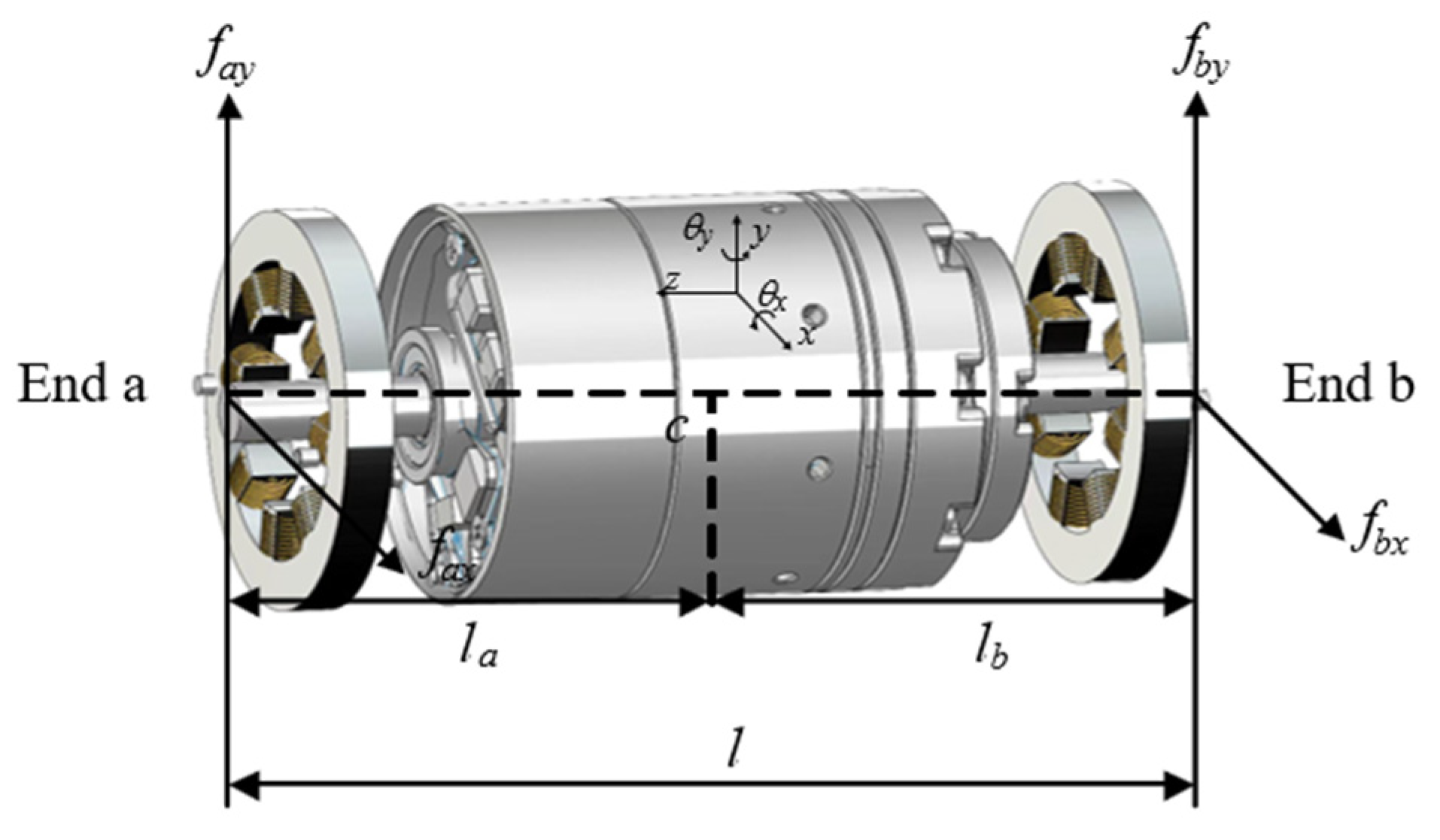
2. Dynamic Modeling of Rigid Rotor System of Electromagnetic Bearing-High Speed Motor

The structure of the rigid rotor system of the AMBs high-speed motor studied in this paper is shown in Figure 1. The axial symmetric rotor is supported by a pair of permanent magnet bearings in the axial direction and two electromagnetic bearings in the radial direction, and the rotor can be regarded as a four-degree-of-freedom rigid rotor system, because the rotor’s operating speed is much lower than the critical speed of the first-order bending.

Figure 1 shows an active magnetic bearings (AMBs) rigid rotor structure, with the cylindrical part at the center being the rigid rotor. At each end of the rigid rotor (End a and End b), there is a set of active magnetic bearings (AMBs). The active magnetic bearings use electromagnetic forces to levitate and control the position of the rotor, allowing it to rotate stably without mechanical contact. Each set of active magnetic bearings consists of several components, of which the key part that generates the electromagnetic force is the magnet windings (the gold-colored coils in the diagram). By applying a current to these windings, a controlled electromagnetic force is generated. f_ax, f_ay, f_bx, and f_by, which represent the electromagnetic force exerted on the rotor by the active magnetic bearings in the x- and y-axis at End a and End b, respectively, are used to accurately control the rotor’s position in both the horizontal and vertical directions and to ensure that the rotor stays stable in suspension and avoids collision and friction with surrounding components. The three-dimensional coordinate axes (x, y, z) in the coordinate axes system diagram are used to define the direction of motion and spatial position of the rotor. θ_x, θ_y represent the rotation angle of the rotor around the x-axis and the y-axis, and the electromagnetic force can be controlled to regulate the rotor’s position and rotation state in all directions, so as to realize the precise control of the rotor. The length parameters l_a and l_b denote the length from the two ends of the rotor to a reference point, respectively, while l denotes the total length of the whole rotor-active magnetic bearing system.

In order to establish the dynamical equations of the radial four-degree-of-freedom AMBs-rigid rotor system for high-speed motors, it is assumed that compared with the rotor mass, the additional unbalance mass of the rotor is very small, which is not enough to affect the offset of the rotor centroid position. The motion state of the unbalanced rotor is still described by the generalized coordinates of the balance rotor centroid C point q = [θy, x, θx, y]^T; due to axis-symmetry, a rigid rotor has the same moment of inertia around the x-axis and around the y-axis; electromagnetic bearings A and B at both ends are not in the same plane as the displacement sensors A and B; the two radial electromagnetic bearings have the same structure and parameters; the influence of axial bearing on the radial motion of rotor is ignored.

Based on the above assumptions, the effects of rotor unbalance and rotor acceleration are considered. Based on the theory of rotor dynamics, the differential equation [21] of motion of the rotor system of the maglev high-speed motor in the process of variable speed motion can be obtained as

$$M\ddot{q}+G\dot{q}-L{u}_f-E_{\epsilon }{F}_{\epsilon }=0,$$

(1)

where $M=diag\left(J,m,J,m\right)$, $q={\left[\begin{array}{cccc}{\theta }_y& x& {\theta }_x& y\end{array}\right]}^{\mathrm{T}}$, $G=\left[\begin{array}{cccc}0& 0& -J_z\omega & 0\\ 0& 0& 0& 0\\ J_z\omega & 0& 0& 0\\ 0& 0& 0& 0\end{array}\right]$, $L=\left[\begin{array}{cccc}{l}_{\mathrm{a}}& -l_{\mathrm{b}}& 0& 0\\ 1& 1& 0& 0\\ 0& 0& -l_{\mathrm{a}}& l_{\mathrm{b}}\\ 0& 0& 1& 1\end{array}\right]$, ${\left.{\mathit{u}}_f=\left[\begin{array}{cccc}{f}_{\mathrm{xa}}& f_{\mathrm{xb}}& f_{\mathrm{ya}}& f_{\mathrm{ya}}\end{array}\right.\right]}^{\mathrm{T}}$, ${\mathit{E}}_{\epsilon }={\left[\begin{array}{cccc}{\mathsf{\epsilon }}_{\mathit{z}}& 1& 0& 0\\ 0& 0& -{\mathsf{\epsilon }}_{\mathit{z}}& 1\end{array}\right]}^{\mathrm{T}}$, ${\mathit{F}}_{\epsilon }=\left[\begin{array}{c}{U}_u({\dot{\varphi }}^2\cos \varphi +\ddot{\varphi }\sin \varphi )\\ U_u({\dot{\varphi }}^2\sin \varphi -\ddot{\varphi }\cos \varphi )\end{array}\right]$. m is the mass of the rotor, ε_z is the projection of the unbalanced mass on the z-axis, ϕ is the angle of rotation, J_z and J are the rotor moment of inertia around the z-axis and around the x-axis (y-axis), respectively; θ_x and θ_y are the angular displacements of the rotor around the x and y axes, respectively. f_ax, f_ay, f_bx and f_ay are the electromagnetic forces on the electromagnetic bearings A and B in the x and y directions, respectively.

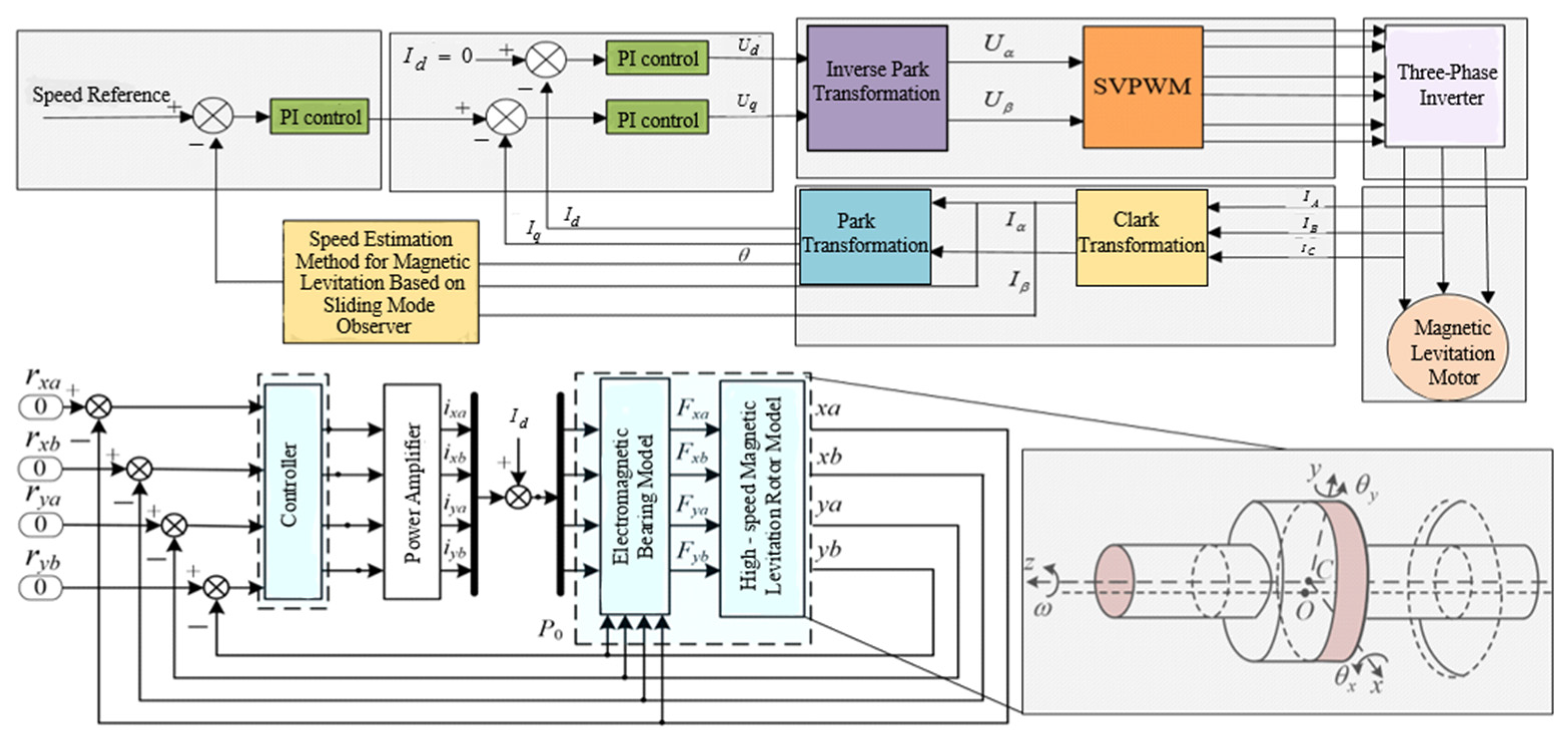
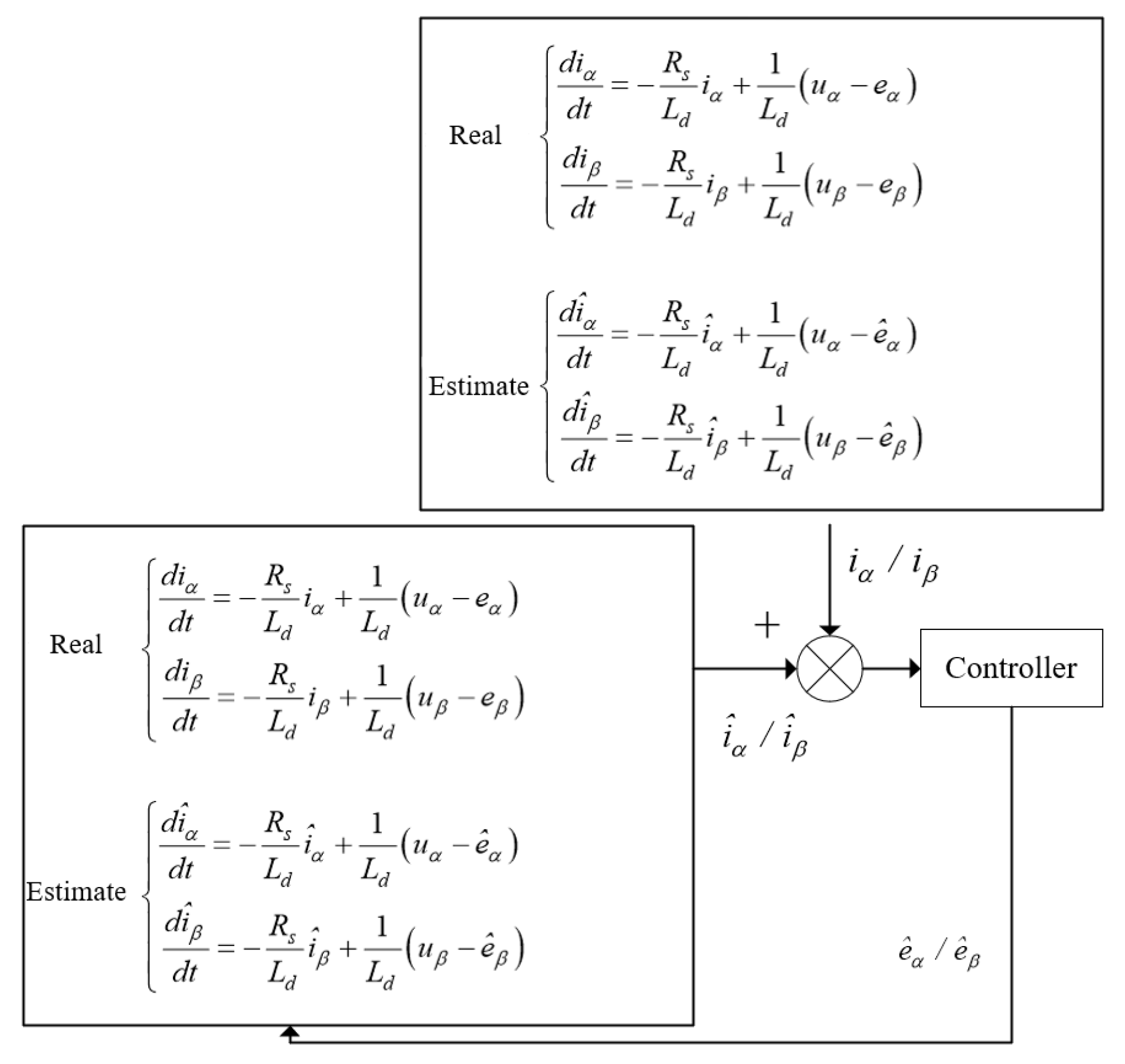
3. Speed Estimation of Maglev Motor Based on Sliding Mode Observer

3.1. Sliding Surface Design

The block diagram of the rotor position control system for magnetic levitation high-speed motor based on sliding mode observer is shown in Figure 2. The control system shown in Figure 2 is divided into two main parts: speed outer loop and current inner loop. In the speed outer loop, the speed reference value is compared with the actual speed value of the motor estimated by the sliding mode observer, and the resulting speed deviation is input to the PI controller for adjustment; at the same time, I_d = 0 is set as the reference value, which is compared with the I_d value calculated by the system and processed by the PI control. In the current inner loop, the outputs of U_d and U_q from the speed loop PI controller are converted into U_α and U_β in the stationary coordinate system by Inverse Park Transformation, where $U\alpha =Ud·\mathrm{c}\mathrm{o}\mathrm{s}\theta - Uq·\mathrm{s}\mathrm{i}\mathrm{n}\theta$ and $U\beta =Ud·\mathrm{s}\mathrm{i}\mathrm{n}\theta +Uq·\mathrm{c}\mathrm{o}\mathrm{s}\theta$, and θ is the electromechanical angle. Then, U_α and U_β are used to generate control signals via Space Vector Pulse Width Modulation (SVPWM) to drive a three-phase inverter to control the operation of the maglev motor. The three-phase currents I_a, I_b, and I_c generated by the motor operation are converted into I_α and I_β in the stationary coordinate system by Clark Transformation, where $I\alpha =Ia$ and $I\beta =(Ia+2Ib)/\sqrt{3}$; subsequently, I_α and I_β are converted into I_α and I_β in the rotating coordinate system by Park Transformation. Iα and Iβ are then converted to I_d and I_q in the rotating coordinate system by Park Transformation, where $Id=I\alpha ·\cos \theta +I\beta ·\sin \theta$ and $Iq=I\beta ·\cos \theta -I\alpha ·\sin \theta ,$ and I_d and I_q are fed back into the system to participate in the control regulation. In the magnetic levitation force control, the reference force in each direction (e.g., F_xa, F_xb, F_ya, and F_yb) is compared with the feedback force values, and the deviation signals are processed by the controller and the power amplifier, which are combined with the electromagnetic bearing model and the high-speed magnetic levitation rotor model, to achieve the precise control of the motor force and ensure that the motor is stably levitated and operates at the desired speed.

The rotor position and speed information of the motor can be accurately calculated from the motor’s inverse electromotive force in the α-β coordinate system. The sliding mode observer has excellent robustness to variations in system parameters as well as to external perturbations. This means that the sliding mode observer maintains its high accuracy and stability even in environments where uncertainty or noise exists. Once the system enters the sliding mode, the characteristics of the sliding mode control allow the observation error to be quickly suppressed and maintained within an acceptable range, which further enhances its reliability and usefulness in practical applications. The actual and estimated current equations [21] are

$$\left\{\begin{array}{c}{\displaystyle \frac{d{i}_{\alpha }}{dt}}=-{\displaystyle \frac{R_s}{L_d}}{i}_{\alpha }+{\displaystyle \frac{1}{L_d}}(u_{\alpha }-e_{\alpha })\\ {\displaystyle \frac{d{i}_{\beta }}{dt}}=-{\displaystyle \frac{R_s}{L_d}}{i}_{\beta }+{\displaystyle \frac{1}{L_d}}(u_{\beta }-e_{\beta })\\ {\displaystyle \frac{d{\widehat{i}}_{\alpha }}{dt}}=-{\displaystyle \frac{R_s}{L_d}}{\widehat{i}}_{\alpha }+{\displaystyle \frac{1}{L_d}}(u_{\alpha }-{\hat{e}}_{\alpha })\\ {\displaystyle \frac{d{\widehat{i}}_{\beta }}{dt}}=-{\displaystyle \frac{R_s}{L_d}}{\widehat{i}}_{\beta }+{\displaystyle \frac{1}{L_d}}(u_{\beta }-{\hat{e}}_{\beta })\end{array}\right.,$$

(2)

where ${\widehat{i}}_{\alpha }$, ${\widehat{i}}_{\beta }$ is the observed stator current, i_α, i_β are the measured currents, R_s is the inter-winding resistance, u_α, u_β are the voltage components in the α-β coordinate system, ${\hat{e}}_{\alpha }$, ${\hat{e}}_{\beta }$ is the estimated reaction potential, e_α, e_β are the reaction potentials, t is the time, and L_d is the d-axis inductance. The current [21] difference is

$$\left\{\begin{array}{c}{\displaystyle \frac{d{\overline{i}}_{\alpha }}{dt}}={\displaystyle \frac{d{\widehat{i}}_{\alpha }}{dt}}-{\displaystyle \frac{d{i}_{\alpha }}{dt}}=-{\displaystyle \frac{R_s}{L_d}}({\widehat{i}}_{\alpha }-i_{\alpha })-{\displaystyle \frac{1}{L_d}}({\hat{e}}_{\alpha }-e_{\alpha })\\ {\displaystyle \frac{d{\overline{i}}_{\beta }}{dt}}={\displaystyle \frac{d{\widehat{i}}_{\beta }}{dt}}-{\displaystyle \frac{d{i}_{\beta }}{dt}}=-{\displaystyle \frac{R_s}{L_d}}({\widehat{i}}_{\beta }-i_{\beta })-{\displaystyle \frac{1}{L_d}}({\hat{e}}_{\beta }-e_{\beta })\end{array}\right.,$$

(3)

This state can be achieved by continuously adjusting the estimated α-β axis reaction potential using the difference in currents. The final control block diagram of the sliding mode observer is obtained as shown in Figure 3. The upper and lower parts of the figure list the actual and estimated α-β-axis current rate of change formulas, respectively. By comparing the actual currents i_α, i_β and the estimated currents, the difference between the two is obtained, and the difference is inputted into the controller. The controller uses the difference value to continuously adjust the estimated α-β-axis counter electromotive force, so that the estimated current gradually approaches the actual current, thus accurately estimating the counter electromotive force of the motor, and then accurately calculating the rotor position and speed information of the motor.

By constantly adjusting the EMF of the α-β axis, the actual α-β axis current is always consistent with the predicted α-β axis current, when the predicted EMF is the actual EMF.

Firstly, it is necessary to define a sliding surface, and then according to the state of the sliding surface to design the control function; according to the predicted α-β axis currents and the actual α-β axis currents to adjust the size of the predicted counter electromotive force, the function [22] S(x) of the sliding surface and its derivatives are selected:

$$S_{\left(x\right)}=\left[{\overline{I}}_{\alpha },{\overline{I}}_{\beta }\right],$$

(4)

$$\dot{S}(x)=\left[{\displaystyle \frac{d{\overline{i}}_{\alpha }}{dt}},{\displaystyle \frac{d{\overline{i}}_{\beta }}{dt}}\right],$$

(5)

Furthermore, it is known that the conditions [22] for the existence of sliding modes are

$$S\dot{S}<0,$$

(6)

Considering the system state space as a two-dimensional plane, where the horizontal coordinates represent the actual state of the system, and the vertical coordinates represent the values of the sliding surface function S. The sliding surface is then a straight line perpendicular to the transverse coordinate, i.e., S = 0. Suppose that initially, the system is at some point (x₀, S₀), and it is hoped that it will arrive at the sliding surface as soon as possible and remain on the sliding surface. The design of a reasonable sliding mode surface makes sure that the system moves towards the sliding surface when S > 0, i.e., the state of the system changes along the direction with negative slope. As the control inputs are applied, the system begins to move in the direction of the decreasing sliding surface function until it finally reaches the sliding surface. At this point, the state of the system satisfies S = 0, i.e., the system is on the sliding surface. Once the system reaches the sliding surface, the controller ensures that $\dot{S}=0$ or $S\ast \dot{S}=0$. Therefore, the control system does not leave the sliding surface but slides steadily along it. Replacing the predicted reverse electromotive force with u(x) [22] gives

$$\left\{\begin{array}{l}{\displaystyle \frac{d{\overline{i}}_{\alpha }}{dt}}=-{\displaystyle \frac{R_s}{L_d}}\left({\overline{i}}_{\alpha }-i_{\alpha }\right)-{\displaystyle \frac{1}{L_d}}\left(u\left(x\right)-e_{\alpha }\right)\\ {\displaystyle \frac{d{\overline{i}}_{\beta }}{dt}}=-{\displaystyle \frac{R_s}{L_d}}\left({\overline{i}}_{\beta }-i_{\beta }\right)-{\displaystyle \frac{1}{L_d}}\left(u\left(x\right)-e_{\beta }\right)\end{array}\right.,$$

(7)

3.2. Rotor Position and Speed Estimation

By adjusting the estimated value of stator current to match the actual value, it can be ensured that the equivalent control component is consistent with the motor’s counter electromotive force, thus realizing the accurate observation and tracking of the motor’s counter electromotive force and ultimately achieving the purpose of observing the counter electromotive force.

Usually, u_eqα and u_eqβ [22] are used as the switching signals for current errors, which not only contain the motor counter electromotive force information but also overlap the high-frequency noise generated by the control strategy.

$$\left\{\begin{array}{l}{u}_{eq\alpha }={\left[-l_{1}sign{\overline{i}}_{\alpha }\right]}_{eq}=e_{\alpha }\\ u_{eq\beta }={\left[-l_{1}sign{\overline{i}}_{\beta }\right]}_{eq}=e_{\beta }\end{array}\right.,$$

(8)

In order to extract the EMF information from the aliased signals, the switching control quantities are usually processed through a low-pass filter to obtain the so-called equivalent control quantities ${\hat{e}}_{\alpha }$ and ${\hat{e}}_{\beta }$ [22], i.e., the motor EMF estimate.

$$\left\{\begin{array}{l}{\hat{e}}_{\alpha }={\displaystyle \frac{{\omega }_0}{{\omega }_0+s}}{u}_{eq\alpha }\\ {\hat{e}}_{\beta }={\displaystyle \frac{{\omega }_0}{{\omega }_0+s}}{u}_{eq\beta }\end{array}\right.,$$

(9)

The low-pass filter cut-off frequency ω₀ is dynamically adjusted according to different rotor speeds. Usually, ω₀ = ω_r/K (K ∊ [1,2]). When the rotor speed changes, the low-pass filter ω₀ needs to be adjusted accordingly in order to keep the system performance optimized. Ensure that an accurate estimate of the motor reaction potential is obtained in time, effectively improving the response speed and stability of the control system. In turn, the estimated rotor position signal [22] can be obtained:

$$\left\{\begin{array}{l}{\hat{e}}_{\alpha }=e_{\alpha }=-{\omega }_r{\psi }_{f}sin\left({\theta }_r\right)\\ {\hat{e}}_{\beta }=e_{\beta }=-{\omega }_r{\psi }_{f}cos\left({\theta }_r\right)\\ {\widehat{\theta }}_r=-\mathit{arc}\mathit{tan}\left({\hat{e}}_{\alpha }/{\hat{e}}_{\beta }\right)\end{array}\right.,$$

(10)

In order to compensate the phase lag caused by low-pass filtering, it is necessary to compensate the phase lag in practical application [23], that is

$$\Delta \theta =\mathit{arc}\mathit{tan}({\omega }^{\prime }/{\omega }_0),$$

(11)

where Δθ is the compensation and ω′ [23] is the observed rotor speed. The estimated motor rotor speed can be obtained as

$${\omega }_r={\omega }^{\prime }=\sqrt{{e_{\alpha }}^2+{e_{\beta }}^2}/{\Psi }_f,$$

(12)

3.3. Stability Analysis

In the design of the maglev control system, in order to ensure that the system can stably enter and remain in the sliding mode region, it is necessary to design a suitable control function u(x) to satisfy the switching surface arrival condition. Regardless of the form of u(x) chosen, the key is to ensure that it satisfies the arrival condition, i.e., to ensure that the state of the system is able to converge to and remain on the slip mode surface according to a predetermined trajectory. Therefore, the design of u(x) must be weighed against the difficulty of its realization and the avoidance of saturation out-of-control phenomenon caused by too large a value, so constant value switching control is chosen [23]:

$$u\left(x\right)=u_{0}sign(S),$$

(13)

where u₀ is the surrogate constant. The constant value function sign(S) [23] is

$$\mathit{sign}\left(S\right)=\left\{\begin{array}{l}1; S>0\\ 0; S=0\\ -1; S<0\end{array}\right.,$$

(14)

The state current equation [23] could be obtained by replacing the predicted EMF with a constant value switching control function with u₀ taken as l₁:

$$\left\{\begin{array}{l}{\displaystyle \frac{d{i}_{\alpha }}{dt}}=-{\displaystyle \frac{R_s}{L_d}}{i}_{\alpha }+{\displaystyle \frac{1}{L_d}}\left(u_{\alpha }-e_{\alpha }\right)\\ {\displaystyle \frac{d{i}_{\beta }}{dt}}=-{\displaystyle \frac{R_s}{L_d}}{i}_{\alpha }+{\displaystyle \frac{1}{L_d}}\left(u_{\beta }-e_{\beta }\right)\end{array}\right.,$$

(15)

Further the current sliding mode observation equation [23] can be obtained:

$$\left\{\begin{array}{c}{\displaystyle \frac{d{\widehat{i}}_{\alpha }}{dt}}=-{\displaystyle \frac{R_s}{L_d}}{\widehat{i}}_{\alpha }+{\displaystyle \frac{1}{L_d}}\left(u_{\alpha }-1,sign\left({\widehat{i}}_{\alpha }-i_{\alpha }\right)\right)\\ {\displaystyle \frac{d{\widehat{i}}_{\beta }}{dt}}=-{\displaystyle \frac{R_s}{L_d}}{\widehat{i}}_{\beta }+{\displaystyle \frac{1}{L_d}}\left(u_{\beta }-1,sign\left({\widehat{i}}_{\beta }-i_{\beta }\right)\right)\end{array}\right.,$$

(16)

To ensure that the sliding mode surface of the sliding mode observer satisfies the condition $S\dot{S}<0$, it is necessary to explore the value of l₁. From the inequality obtained before, (17) [23] is obtained as

$$\begin{array}{l}{\overline{i}}_{\beta }{\dot{\overline{i}}}_{\beta }={\overline{i}}_{\beta }\left(-{\displaystyle \frac{R_s}{L_d}}{\overline{i}}_{\beta }+{\displaystyle \frac{e_{\beta }}{L_d}}-{\displaystyle \frac{l_1}{L_d}}\mathit{sign}{\overline{i}}_{\beta }\right)\\ =-{\displaystyle \frac{R_s}{L_d}}{{\overline{i}}_{\beta }}^2+{\displaystyle \frac{e_{\beta }{\overline{i}}_{\beta }}{L_d}}-{\displaystyle \frac{l_1}{L_d}}\mathit{sign}\left({\overline{i}}_{\beta }\right){\overline{i}}_{\beta }\\ =\left\{\begin{array}{l}{\displaystyle \frac{1}{L_d}}{\overline{i}}_{\beta }\left(e_{\beta }-l_1\right)-{\displaystyle \frac{R_s}{L_d}}{{\overline{i}}_{\beta }}^2; {\overline{i}}_{\beta }>0\\ {\displaystyle \frac{1}{L_d}}{\overline{i}}_{\beta }\left(e_{\beta }{+l}_1\right)-{\displaystyle \frac{R_s}{L_d}}{{\overline{i}}_{\beta }}^2; {\overline{i}}_{\beta }<0\end{array}\right.,\end{array}$$

(17)

The sliding mode arrival condition in the designed sliding mode function [23] is, i.e., the following condition demands to be satisfied as

$$\left\{\begin{array}{l}{i}_{\alpha }{\widehat{i}}_{\alpha }<0\\ i_{\beta }{\widehat{i}}_{\beta }<0\end{array}\right.,$$

(18)

Through the above analysis, it can be found that only when the formula l₁ > max (|e_α|, |e_β|) is satisfied, all the above conditions can be satisfied, which makes the error equation gradually converge to stability. However, the value of l₁ needs to be considered in practical applications; if the value of l₁ is taken too large, it will increase the jitter noise of the motor and cause estimation errors in the system. This control strategy starts to play a key role at the point where the system enters the sliding mode phase, once the sliding surface variable is zeroed out, and the system will rely on an equivalent control mechanism to maintain its continuous sliding state on the sliding surface.

When designing SMO-based velocity estimation methods for magnetic levitation motors, it is crucial to ensure the stability of the system under multiple uncertainty conditions. Sliding mode control, by virtue of its inherent robustness, is able to effectively cope with the effects of external perturbations, parameter variations and unmodelled dynamics. However, the asymptotic stability of the system needs to be explored in depth in the presence of chattering effect, stator resistance variation, and critical speed bending mode.

The essence of sliding mode control is to drive the system state towards the sliding mode surface by relying on discontinuous control laws. However, this type of control triggers high frequency switching phenomena near the sliding mode surface, which in turn leads to chattering effects and makes the control signal fluctuate violently. In order to deeply analyze the stability of the system in this case, the Lyapunov function [24] is defined as

$$V(S)={\displaystyle \frac{1}{2}}{S}^2,$$

(19)

The derivation of the equation [24] is obtained:

$$\dot{V}=S\dot{S},$$

(20)

The results of the derivation are obtained by substituting into Equation (13) in conjunction with the sliding mold surface arrival condition [24]:

$$\dot{V}=u_0\left|u\left(x\right)\right|,$$

(21)

where u₀ > 0 and hence $\dot{V} \le 0$, indicating that the system is able to ensure global asymptotic stability. This means that even in the presence of chattering, the system state will still converge to the slipmould surface in finite time and remain stable in that region without divergence.

During the actual operation of the motor, the stator resistance R_s is affected by a variety of factors, such as temperature drift, material aging, etc., and thus changes. This change will have a direct impact on the current observation error [23]. We define the current error as

$$\left\{\begin{array}{l}{\tilde{i}}_{\alpha }=i_{\alpha }-{\widehat{i}}_{\alpha }\\ {\tilde{i}}_{\beta }=i_{\beta }-{\widehat{i}}_{\beta }\end{array}\right.,$$

(22)

Then, its dynamic equation can be expressed as [23]

$${\displaystyle \frac{d{\tilde{i}}_{\alpha }}{dt}}=-{\displaystyle \frac{(R_s+\Delta R_s)}{L}}{\tilde{i}}_{\alpha }+{\displaystyle \frac{\Delta R_s}{L}}{i}_{\alpha },$$

(23)

In order to analyze the stability of the system in this case, we choose the Lyapunov function as [24]

$$V(\tilde{i})={\displaystyle \frac{1}{2}}({\tilde{i}}_{\alpha }^2+{\tilde{i}}_{\beta }^2),$$

(24)

Derivation of this equation yields [23]

$$\dot{V}=-{\displaystyle \frac{(R_s+\Delta R_s)}{L}}({\tilde{i}}_{\alpha }^2+{\tilde{i}}_{\beta }^2)+{\displaystyle \frac{\Delta R_s}{L}}(i_{\alpha }{\tilde{i}}_{\alpha }+i_{\beta }{\tilde{i}}_{\beta }),$$

(25)

When $\left|\Delta Rs\right|$ is small, the first term dominates, making $\dot{V}\le 0$, indicating that the system still has asymptotic stability. As long as the stator resistance changes within a certain range, the stability of the system will not be fundamentally damaged but will continue to converge to the sliding mode surface and maintain stable operation.

A non-negligible problem that arises when the motor is in high-speed operation is that the rotor may enter a bending mode. The emergence of such a mode can lead to significant changes in the magnetic axis bearing force, which in turn can have a serious impact on the accuracy of the speed estimation. Assuming that there is an unmodelled dynamic disturbance term d(t) acting on the system, the error dynamics equation of the system can then be expressed as [23]

$${\displaystyle \frac{d\tilde{i}}{dt}}=-{\displaystyle \frac{R_s}{L}}\tilde{i}+{\displaystyle \frac{1}{L}}(u-e)+d(t),$$

(26)

In order to study the stability of the system in this case, the Lyapunov function is chosen as [24]

$$V={\displaystyle \frac{1}{2}}{\tilde{i}}^2,$$

(27)

The derivatives of the above equations are obtained [23]:

$$\dot{V}=-{\displaystyle \frac{R_s}{L}}{\tilde{i}}^2+{\displaystyle \frac{1}{L}}d(t)\tilde{i},$$

(28)

If d(t) is bounded and its value is sufficiently small, then the first term of Equation (28) will dominate the behavior of the system in this equation such that $\dot{V}\le 0$. This implies that the system remains asymptotically stable even in the presence of such perturbations.

By performing in-depth stability proofs for the three cases mentioned above, we can clearly see that the sliding mode observer is able to maintain the asymptotic stability of the system in the face of complex and intractable operating conditions such as chattering effects, stator resistance variations, and unmodelled dynamics.

4. Emulation Analysis

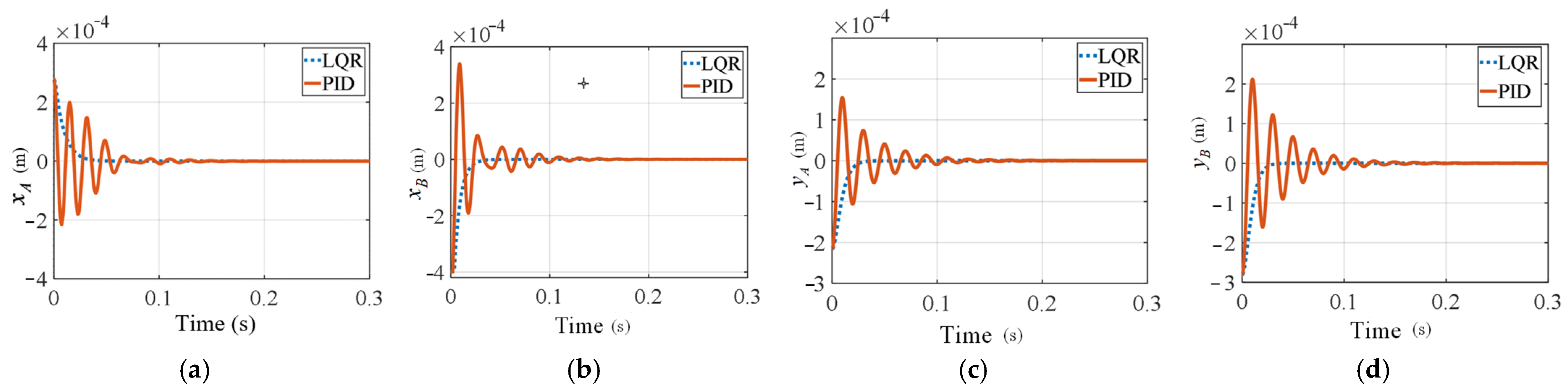
4.1. Verification of Motor Floating Operation

We used Simulink software (24.2) in MATLAB, version MATLAB R2024b. In this simulation, we mainly utilized the following functions and modules: electrical system module library, control module library, and also built coordinate transformation modules (e.g., Clark transformation, Park transformation, and its inverter module) to complete the conversion of electrical quantities in different coordinate systems.

Figure 4 gives the waveforms of the AMBs-high-speed motor rigid rotor system at both ends in the $x_A$, $x_B$, $y_A$ and $y_B$ directions of the gravity. As can be seen from Figure 4, whether the main controller of the system adopts PID controller or LQR controller, the four-degree-of-freedom rotor can be stably suspended in the central position after 0.1 s. In the dynamic adjustment process of stable suspension of the rotor, the maximum vibration is 0.35 mm, which is less than 0.4 mm unilateral protection gap.

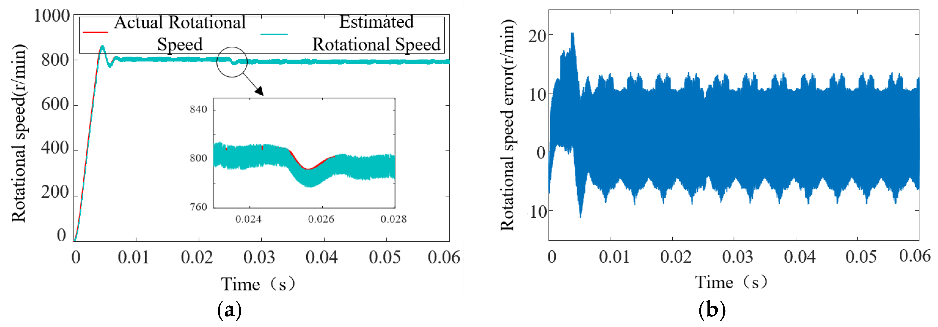
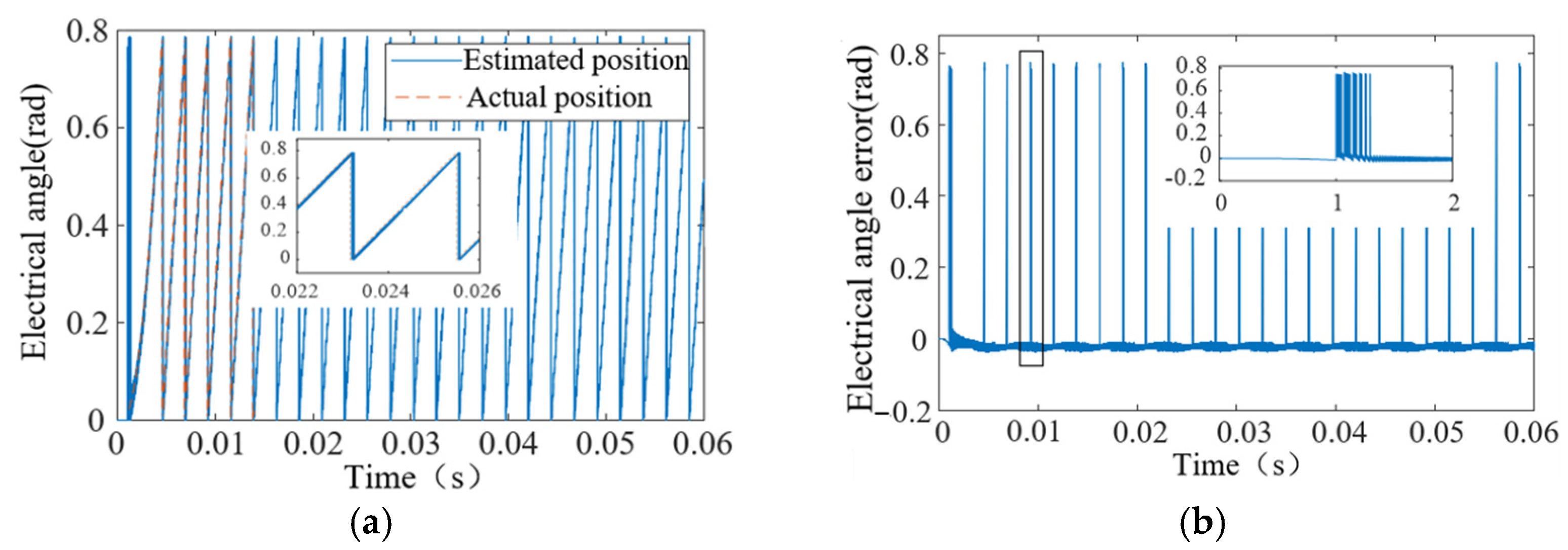
4.2. Verification of Speed Estimation Based on Sliding Mode Observer

Figure 5a shows a plot of estimated speed versus actual speed for a magnetic levitation high-speed motor based on a sliding mode observer. When the maglev motor is running at a given speed of 800 r/min, it can be seen that the maximum error between the actual speed and the estimated speed is less than 20 r/min, with a percentage error of 2.5%. The analysis of the speed response curve shows that the estimated speed of the magnetic levitation motor reaches the given value within 2 ms with a maximum overshoot of 55 r/min and an overshoot percentage of 6.8%. The small overshoot and high steady-state accuracy of the electric power from start-up to operation to a given speed indicate that the magnetic levitation motor system has good static and dynamic performance. Meanwhile, in order to verify the loading characteristics of the system, the motor was given a sudden increase in load at 0.025 s, and the motor speed dropped and then quickly recovered to the given speed, which demonstrated the system’s good immunity to load changes.

Figure 6a gives a plot of the estimated rotor position versus the actual rotor position curve of the magnetic levitation high-speed motor based on the sliding mode observer. It can be seen that the estimated position curve coincides almost exactly with the actual position curve, which indicates that the deviation between the two is extremely small. In addition, as shown in Figure 6b, the difference between the actual position and the estimated position also remains low, further demonstrating the accuracy of the sliding mode observer in position estimation. It is worth noting that after the motor is loaded abruptly at the 0.025 s moment, the estimated position is still able to follow the change in the actual position quickly despite the presence of external perturbations, which indicates that the sliding mode observer has fast convergence characteristics and anti-perturbation capability.

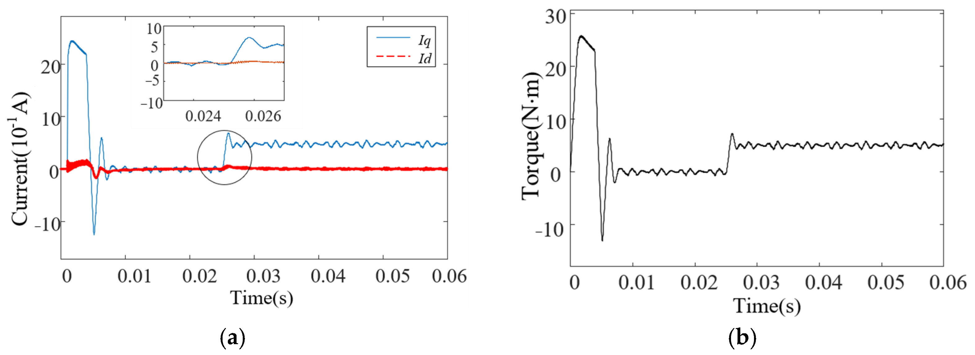
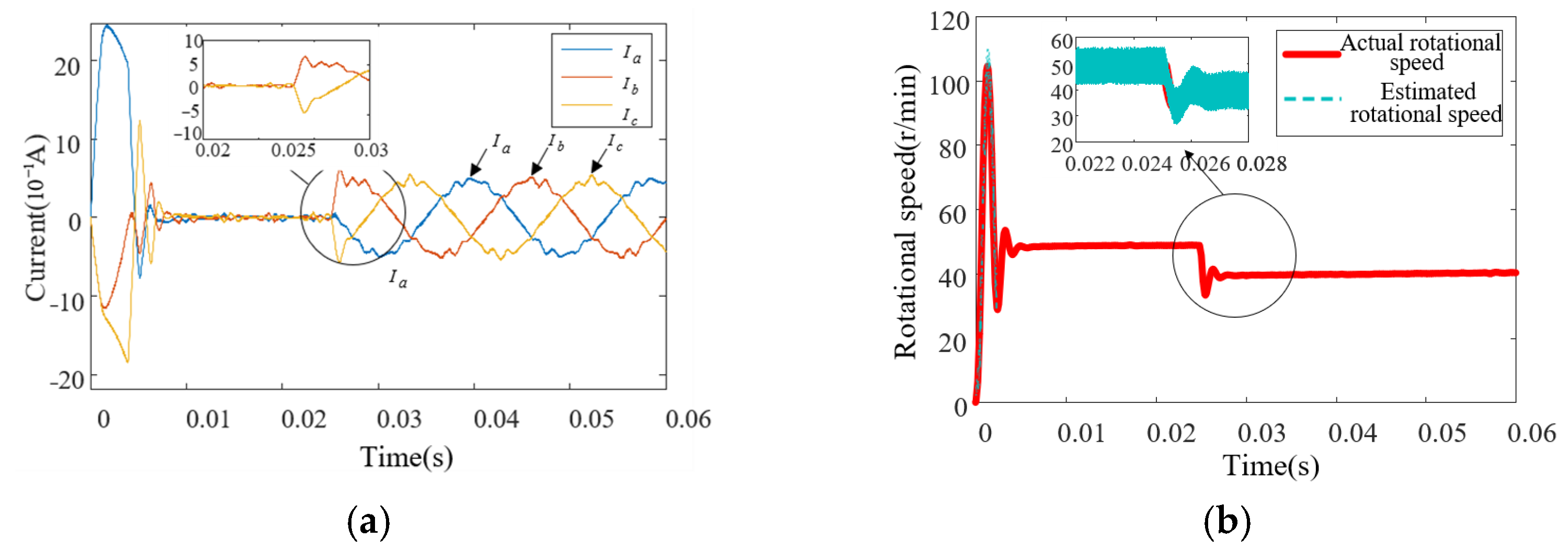
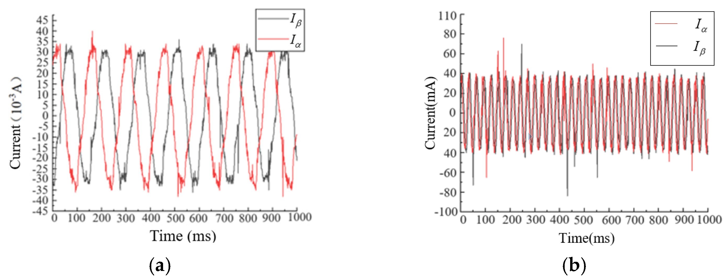
4.3. Verification of Motor Current and Torque

The stator magnetic chain orientation method, i.e., i_d = 0 vector control strategy, is used for simulation and experiment. As can be seen in Figure 7a, both i_d and i_q fluctuate after a sudden load is applied to the maglev rotor at 5 ms, and i_q quickly reaches 25 A within a short period of 5 ms. Subsequently, after 2 ms of rapid regulation, the i_d and i_q waveforms tend to be stable and basically remain near 0 A, which verifies the rapidity of the current regulation of the magnetic levitation motor. The rapid rise in torque to peak values during the start-up phase of the maglev motor shows that the speed regulator responds quickly and accelerates the torque to its maximum value after reaching saturation. Once the motor speed reaches the preset value, the torque drops back quickly and remains stable, a performance that demonstrates the fast response of the system during the start-up phase.

In the i_d = 0 control mode, torque control is essentially control of i_q, i.e., there is a positive relationship between i_q and torque. At 0.025 s, the system applies a load. In response to disturbances, the torque output is able to increase quickly to match the load size. This performance verifies that the system has excellent disturbance resistance and fast adjustment capability, ensuring that the motor can still maintain stable operation when the load changes.

The three-phase current waveform of the motor is shown in Figure 8a, indicating that the current waveform varies greatly at the instant of motor startup, and then tends to stabilize as a whole, and the three-phase current of the motor oscillates slightly after the load is applied for 0.025 s, but it soon tends to stabilize, which again verifies the system’s disturbance-resistant performance.

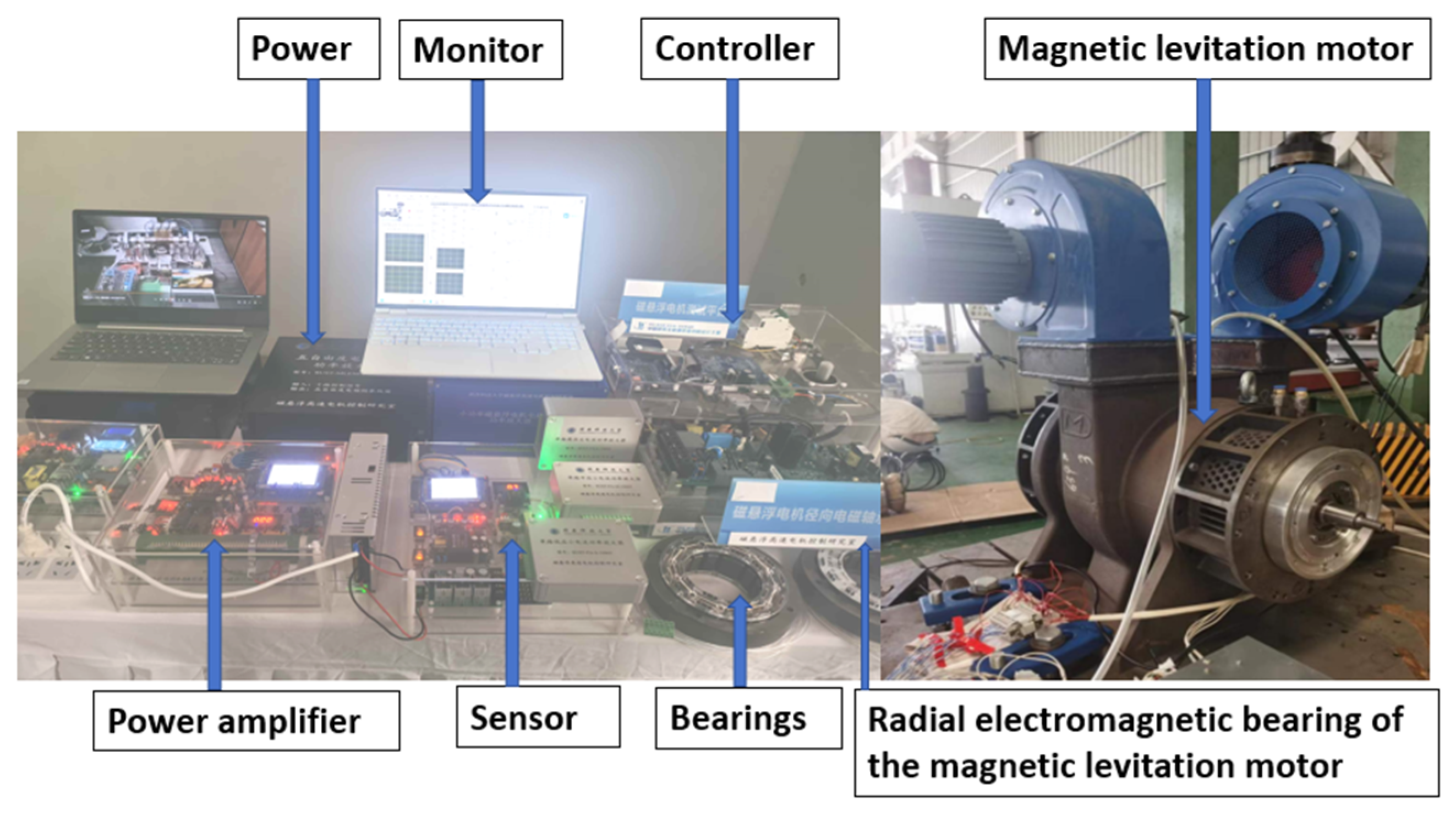
5. Experimental Verification

The experimental setup is shown in Figure 9, where the power supply powers the device, the power amplifier receives signals from the controller and amplifies them, and the sensors use eddy current sensors to measure rotor displacement in order to collect data in real time during the operation of the magnetic levitation motor. The controller consists of a DSP28335-based driver board, which is responsible for processing the data from the sensors and generating the corresponding control signals according to a preset control algorithm. The display is connected to the software of the upper computer and is used to display the data collected and transmitted from the experimental equipment in real time. In this experiment, considering the actual data processing capability and signal characteristics, a sampling rate of 20 kHz is selected, and a low-pass filter with a cut-off frequency of 3 kHz is used to process the collected signals. The sensitivity of the displacement sensor is 10 V/mm, and the maximum output current of the power amplifier is 10 A.

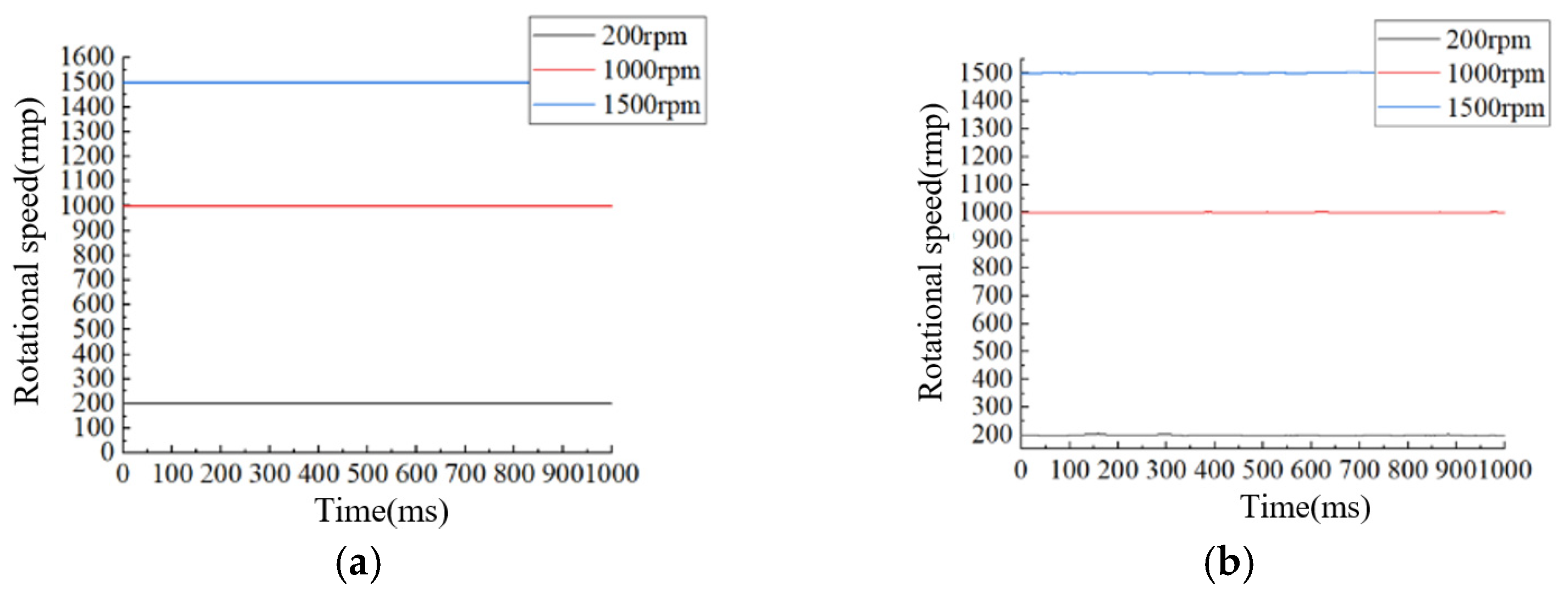
5.1. Observation of Motor Speed Under No-Load

The waveforms of the speed estimation of the sliding mode observer are given in Figure 10a. The given rotational speeds of the magnetic levitation motor are set as 200 rpm, 1000 rpm, and 1500 rpm, and the estimated rotational speeds are shown in Figure 10b. As shown in Figure 11, at 200rpm and 1000rpm, the amplitudes of the current waveforms of $I_{\alpha }$ and $I_{\beta }$ after the Clark transformation are almost the same. The higher the rotational speed, the faster the Clark transformation. The reason is that the rotational speed of the motor is directly related to the frequency of the three-phase voltage or current signals it generates. It can be seen that the speed estimation value obtained by the sliding mode observer is very close to the given value and can correctly feedback the actual speed of the motor, which verifies the feasibility of the rationale and the correctness of the simulation.

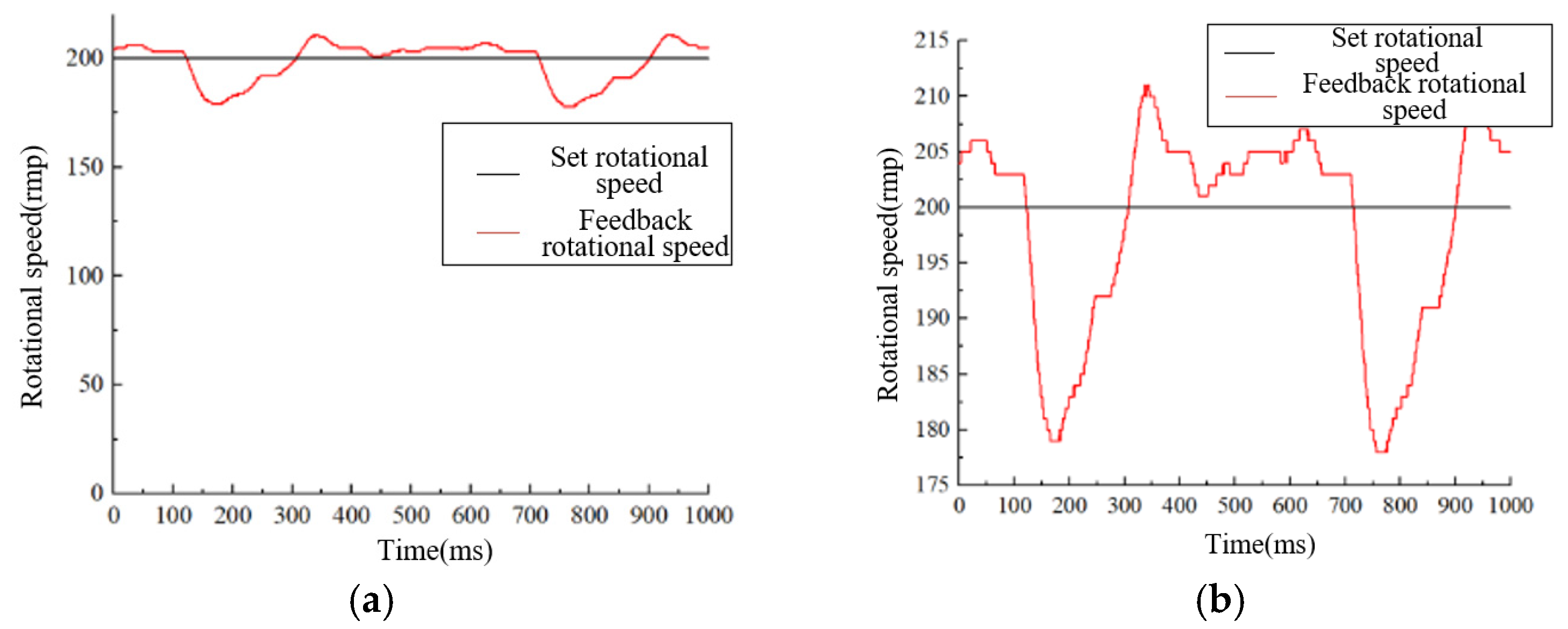
5.2. Observation of Motor Speed During Loading

In the experiment of the double closed-loop control system of a MLM based on the sliding mode observer method, Figure 12 shows the set speed and the feedback speed of the system with a sudden load when the given speed is 200 rpm, and it can be seen from the figure that the speed fluctuates when the load is increased, but they are all stable in the range of the set speed, and the difference in the speed fluctuation after the application of the load can be found to be between 20 rpm at most through the local zoomed-in diagram, and the steady-state fluctuation can be up to 10%, which is consistent with the theoretical analysis. Up to 10%, this result is consistent with the theoretical analysis, the sliding mode observer in the motor running at a lower speed when the estimation error and dynamic performance is poor.

Therefore, in order to verify that the sliding mode observer is suitable for higher speed conditions, the motor running speeds are set to 1200 rpm and 1500 rpm, respectively. When the load is suddenly applied, the dynamic response waveforms of the motor speed are given in Figure 13 and Figure 14, which show that when the motor is running at 1200 rpm, the maximum error difference in the rotational speed is 10 rpm, with the steady-state fluctuation lower than 1%; when the motor is running at 1500 rpm, the maximum speed error difference is 20 rpm, and the steady state fluctuation is lower than 1.5%.

5.3. Acceleration and Deceleration Experiments

The response curves of the rotor levitation experiments with multiple degrees of freedom in terms of voltage variation with time are presented in Figure 15. The first four curves represent the voltage changes in the radial direction (AX, BX, BY, AY), while the last curve corresponds to the axial (Z) direction. The horizontal axis represents time (1 ms per cell), and the vertical axis represents voltage (2 volts per cell). Each curve is labeled with the maximum voltage (U_max), minimum voltage (U_min) and average voltage (U_avg) in order to capture the dynamic characteristics in each direction. During the initial phase (0 ms to 3.7 ms), the rotor is in its natural state with no bias voltage applied and the voltage curves in each direction remain relatively stable.

The bias voltage is applied at 3.7 ms to initiate the rotor motion, and the radial voltage curves (AX, BX, BY, AY) show significant jumps, and the rotor reaches a stable suspension state at about 7 ms, which is manifested by the voltage amplitude leveling off. The bias voltage is removed at 10.75 ms, and the rotor returns to its natural state, and the voltages in each direction are restored to the initial conditions. The axial response trend is similar to that of the radial direction, but with minor differences: the bias voltage triggers the axial motion at 3.7 ms, the rotor reaches a stable levitation state at 5.7 ms, and the axial voltages return to the initial condition just as quickly after the bias voltage is removed. Critical time intervals (e.g., 3.3 ms for radial stabilization and 2 ms for axial stabilization) and state transition points are highlighted in the figure. The experimental results verify the dynamic response characteristics of the rotor transitioning from the natural state to the levitated state under controlled conditions, indicating that the system is capable of stable levitation with multiple degrees of freedom.

Figure 16a shows the vibration signals of a four-degree-of-freedom rotor operating at 45,000 revolutions per minute under magnetic levitation. The vibration response of the rotor along the radial direction (AX, BX, BY, AY) and axial direction (Z) during the acceleration and deceleration phases is depicted in the figure. The vibration amplitudes are expressed in volts and each curve is labeled with maximum vibration amplitude (U_max), minimum vibration amplitude (U_min) and average vibration amplitude (U_avg), and a uniform scale of 2 volts/gram is used for all signals.

In the radial direction, the initial stage shows transient vibration caused by start-up instability, and the vibration amplitude gradually tends to stabilize with the increase in speed, indicating that the rotor has reached the steady-state operating condition; in the deceleration stage, the vibration amplitude increases again due to the destabilizing effect of rotor inertia and desynchronization. In contrast, the axial vibration has a relatively small amplitude during the whole operation process, which is due to the fact that the magnetic levitation system effectively compensates for the gravity force on the horizontally aligned rotor, thus ensuring the uniformity and consistency of the axial force. The error between the rotor vibration and the neutral point is shown in Figure 16b, according to which it can be calculated that the system has a lower root mean square error and a higher signal-to-noise ratio, which concludes that the system has a higher accuracy of speed estimation and better noise immunity, which is more advantageous.

6. Discussion

In the process of constructing the velocity model based on the adaptive sliding mode observer, the computational complexity is mainly concentrated in the design of the sliding mode surface. The sliding mode surface design needs to determine the sliding mode surface function, and its derivatives based on the motor’s reverse electromotive force, actual, and estimated current equations in the α-β coordinate system. The experimental platform is constructed based on the DSP28335 driver board (Operating frequency: 20 kHz), the AD sampling time is longer than the DSP calculation period, so there is no lag in the sampling process. However, its processing capability is limited, and the processing delay may occur when facing complex calculations, resulting in untimely speed estimation, especially when the motor is loaded or the speed changes abruptly, the system response is lagging, which seriously affects the motor control accuracy. However, the DA output in the power amplifier part may have a lag, because the DA chip needs to complete five current outputs, but also a series of signal processing circuits, so it will bring some lag to the system. To solve this problem, phase compensators can be connected in series in the control loop to compensate for the system lag due to calculation or other factors.

In addition, speed estimation faces many challenges. When approaching zero speed, the motor reverse electromotive force signal is weak and the signal-to-noise ratio is low, which interferes with the accurate observation of the reverse electromotive force by the sliding mode observer and affects the accuracy and stability of speed estimation. During the operation of the maglev motor, the initial rotor misalignment generates an unbalanced magnetic pull, which exacerbates the vibration of the motor and affects normal operation. Meanwhile, once the sensors and actuators, which are important components of the system, fail, such as the failure of the displacement sensor, the control system will not be able to obtain accurate position feedback information, leading to the failure of the velocity estimation method based on position feedback. If the actuator fails, it may cause the electromagnetic force to lose balance, which will cause the rotor to lose stability and collide with the protection bearing, which can cause the rotor and the protection bearing to be damaged in serious cases.

To address the above problems, there is still room for improvement in this study. Optimization at the algorithmic level can simplify the design of the sliding mode surface and the signal calculation process to reduce the computational complexity, in order to adapt to hardware with limited processing capability such as DSP28335; for the observation of the inverse electromotive force at low rotational speeds, new signal processing and filtering algorithms can be explored to improve the quality of the signals; for the problem of rotor misalignment, advanced on-line monitoring and auto-correction techniques can be developed to guarantee the stable operation of the motor, thus enhancing the speed estimation of magnetic levitation motors. Thus, the accuracy of the speed estimation of the maglev motor and the performance of the whole system can be improved.

7. Conclusions

In this study, the rotational speed of a maglev motor is estimated. In constructing the dynamics model of the rigid rotor system of the maglev motor, many unique factors of the maglev motor/active magnetic bearing (MLM/AMB) system are fully considered, and the relevant specific planes and coordinate systems are defined to pay attention to the additional unbalanced mass of the rotor, the positional relationship between the electromagnetic bearings and displacement sensors, etc., so that the constructed differential equations of motion are able to accurately describe the system’s motion state. Based on this accurate model, this study further optimizes the slip mold surface design and speed estimation algorithm. Using the connection between the motor’s reverse electromotive force in the α-β coordinate system and the rotor position and rotational speed, a specific slip mode surface function and its derivatives are designed by combining the actual current equation and the estimated current equation. During the speed estimation process, the low-pass filter cutoff frequency ω₀ is dynamically adjusted according to the rotor speed and compensated for the phase lag, which greatly improves the system performance.

The SMO-based rotational speed estimation method proposed in this study has significant advantages in magnetic levitation systems, which makes it a very promising application scenario in several fields. In maglev train operation, the method can accurately obtain the motor speed information in real time and accurately regulate the train speed to ensure that the train remains smooth at high speed. Moreover, it is highly robust to changes in motor parameters and external disturbances, which can reduce maintenance costs and extend the service life of the equipment. In the aerospace field, for the magnetic levitation bearing system of aviation engines, the method can accurately estimate the motor speed, achieve stable levitation and high-speed rotation control of the engine rotor, improve the efficiency and performance of the engine, and reduce friction and wear, energy consumption and noise pollution. In the field of industrial production, the magnetic levitation spindle system of high-precision machining equipment adopts this method, which can monitor and control the spindle speed in real time to guarantee the stability and precision of machining.

References

1. Jiang, H.; Su, Z.; Wang, D. Analytical Calculation of Active Magnetic Bearing Based on Distributed Magnetic Circuit Method. IEEE Trans. Energy Convers. 2020, 36, 1841–1851. [Google Scholar] [CrossRef]
2. Gong, L.; Yang, Z.; Zhu, C.; Li, P. Automatic Balancing of Rigid Rotor for Magnetic Levitation High-Speed Motor Based on Polarity Switching Adaptive Trap. J. Electrotechnol. 2020, 35, 1410–1421. [Google Scholar]
3. Zhang, D.; Jiang, J.; Wang, B. Multisource Oscillation Suppression Control of Magnetic Levitation High-Speed Permanent Magnet Motor. IEEE Access 2022, 10, 106506–106512. [Google Scholar] [CrossRef]
4. Ozturk, U.K.; Abdioglu, M.; Ozkat, E.C.; Mollahasanoglu, H. Extended 2-D Magnetic Field Modeling of Linear Motor to Investigate the Magnetic Force Parameters of High-Speed Superconducting Maglev. IEEE Trans. Appl. Supercond. 2023, 33, 1–8. [Google Scholar] [CrossRef]
5. Liao, Z.; Yue, J.; Lin, G. Application Research of HTS Linear Motor Based on Halbach Array in High-Speed Maglev System. IEEE Trans. Appl. Supercond. 2021, 31, 1–7. [Google Scholar] [CrossRef]
6. Saeed, N.A.; Awwad, E.M.; El-Meligy, M.A.; Nasr, E.S.A. Radial versus Cartesian Control Strategies to Stabilize the Nonlinear Whirling Motion of the Six-Pole Rotor-AMBs. IEEE Access 2020, 8, 138859–138883. [Google Scholar] [CrossRef]
7. Wu, H.; Yu, M.; Song, C.; Wang, N. Unbalance Vibration Suppression of Maglev High-Speed Motor Based on the Least-Mean-Square. Actuators 2022, 11, 348. [Google Scholar] [CrossRef]
8. Li, J.; Ma, X. Vibration Mechanism and Compensation Strategy of Magnetic Suspension Rotor System Under Unbalanced Magnetic Pull. IEEE Access 2022, 10, 31235–31243. [Google Scholar]
9. Le, Y.; Wang, D.; Zheng, S. Design and Optimization of a Radial Magnetic Bearing Considering Unbalanced Magnetic Pull Effects for Magnetically Suspended Compressor. IEEE/ASME Trans. Mechatron. 2022, 27, 5760–5770. [Google Scholar] [CrossRef]
10. Gong, L.; Zhu, C. Coincident Vibration Suppression of Rigid Rotor of Magnetic Levitation High-Speed Motor Based on Four-Factor Variable Polarity Control. Chin. J. Electr. Eng. 2021, 41, 1515–1524. [Google Scholar]
11. Yao, C.; Zhou, Y. Active Disturbance Rejection and Ripple Suppression Control Strategy with Model Compensation of Single-Winding Bearingless Flux-Switching Permanent Magnet Motor. IEEE Trans. Ind. Electron. 2022, 69, 7708–7719. [Google Scholar]
12. Li, Y.; Hu, Y.; Zhu, Z.Q. Current Harmonics and Unbalance Suppression of Dual Three-Phase PMSM Based on Adaptive Linear Neuron Controller. IEEE Trans. Energy Convers. 2023, 38, 2353–2363. [Google Scholar] [CrossRef]
13. Zhou, T.; Zhu, C. Design of Robust Output Feedback Controllers for Rigid Rotor Systems of High-Speed Motors with Electromagnetic Bearings Based on Feature Structure Configurations. Chin. J. Electr. Eng. 2022, 42, 3775–3786. [Google Scholar]
14. Cao, Z.; Huang, Y.; Peng, F.; Dong, J. Driver Circuit Design for a New Eddy Current Sensor in Displacement Measurement of Active Magnetic Bearing Systems. IEEE Sens. J. 2022, 22, 16945–16951. [Google Scholar] [CrossRef]
15. Hutterer, M.; Schroedl, M. Stabilization of Active Magnetic Bearing Systems in the Case of Defective Sensors. IEEE/ASME Trans. Mechatron. 2021, 27, 3672–3682. [Google Scholar] [CrossRef]
16. Yu, K.; Wang, Z. Position Sensorless Control of IPMSM Using Adjustable Frequency Setting Square-Wave Voltage Injection. IEEE Trans. Power Electron. 2022, 37, 12973–12979. [Google Scholar] [CrossRef]
17. Liu, Z.-H.; Nie, J.; Wei, H.-L.; Chen, L.; Li, X.-H.; Lv, M.-Y. Switched PI Control Based on MARS for Sensorless Control of PMSM Drives Using Fuzzy-Logic-Controller. IEEE Open J. Power Electron. 2022, 3, 368–381. [Google Scholar] [CrossRef]
18. Wang, Z.; Yu, K.; Li, Y.; Gu, M. Position Sensorless Control of Dual Three-Phase IPMSM Drives with High-Frequency Square-Wave Voltage Injection. IEEE Trans. Ind. Electron. 2022, 70, 9925–9934. [Google Scholar] [CrossRef]
19. Zhang, Y.; Yin, Z.; Tang, R.; Liu, J. Moment of Inertia and Load Torque Identification Based on Adaptive Extended Kalman Filter for Interior Permanent Magnet Synchronous Motors. IEEE Trans. Instrum. Meas. 2025, 74, 1–12. [Google Scholar] [CrossRef]
20. Zhang, L.; Li, S. Performance Analysis of High-Frequency Signal Injection Methods for Sensorless Control of PMSM in Low-Speed Range. Sensors 2021, 21, 1234. [Google Scholar]
21. Gong, L.; He, P.; Yichen, W.; Zhaoyang, D.; Zhu, C. Vibration Control of Full Rotational Speed Range for Magnetically Levitated High-Speed Motors Based on Linear Quadratic Regulator. J. Vib. Eng. Technol. 2025, 13, 97. [Google Scholar] [CrossRef]
22. Liang, J.; Wu, J.; Wang, Y.; Zhong, Z.; Bai, X. Sensorless Control for a Permanent Magnet Synchronous Motor Based on a Sliding Mode Observer. Eng 2024, 5, 1737–1751. [Google Scholar] [CrossRef]
23. Liu, W.; Luo, B.; Yang, Y.; Niu, H.; Zhang, X.; Zhou, Y.; Zeng, C. An Adaptive-Gain Sliding Mode Observer with Precise Compensation for Sensorless Control of PMSM. Energies 2023, 16, 7968. [Google Scholar] [CrossRef]
24. Park, S.; Ban, J.; Doh, S. Hybrid Reaching Law of Sliding Mode Position-Sensorless Speed Control for Switched Reluctance Motors. Electronics 2025, 14, 577. [Google Scholar] [CrossRef]
Figure 1. AMBs-rigid rotor structure.
Energies 18 01539 g001
Figure 2. Block diagram of rotor control system based on SMO for MLM.
Energies 18 01539 g002
Figure 3. Control block diagram of the sliding mode observer.
Energies 18 01539 g003
Figure 4. The position of both ends of the rotor suspension. (a) xA. (b) xB. (c) yA. (d) yB.
Energies 18 01539 g004
Figure 5. The motor rotor speed. (a) Estimated speed and actual speed. (b) Rotor speed error.
Energies 18 01539 g005
Figure 6. The motor rotor position. (a) Estimated speed and actual position. (b) Rotor position error.
Energies 18 01539 g006
Figure 7. Waveform. (a) id, iq waveforms. (b) Torque waveform.
Energies 18 01539 g007
Figure 8. 3-phase current waveform and estimation speed of 50 rpm. (a) 3-phase current waveform. (b) Estimation speed of 50 rpm.
Energies 18 01539 g008
Figure 9. Experimental rig.
Energies 18 01539 g009
Figure 10. The motor speed. (a) Set speed. (b) Feedback speed.
Energies 18 01539 g010
Figure 11. Iα, Iβ waveforms. (a) Iα. (b) Iβ.
Energies 18 01539 g011
Figure 12. Motor rotational speed in the case of 200 rpm. (a) Set and feedback speed. (b) Enlarged plot.
Energies 18 01539 g012
Figure 13. Motor rotational speed in the case of 1200 rpm. (a) Set and feedback speed. (b) Enlarged plot.
Energies 18 01539 g013
Figure 14. Motor rotational speed in the case of 1500 rpm. (a) Set and feedback speed. (b) Enlarged plot.
Energies 18 01539 g014
Figure 15. Time plot of rotor axial and radial voltage fluctuations.
Energies 18 01539 g015
Figure 16. Plot of rotor vibrations. (a) Plot of rotor axial and radial speed voltage vibrations and feedback speed. (b) Plot of rotor vibration error diagram.
Energies 18 01539 g016
Disclaimer/Publisher’s Note: The statements, opinions and data contained in all publications are solely those of the individual author(s) and contributor(s) and not of MDPI and/or the editor(s). MDPI and/or the editor(s) disclaim responsibility for any injury to people or property resulting from any ideas, methods, instructions or products referred to in the content.