2.1. Fault Identification
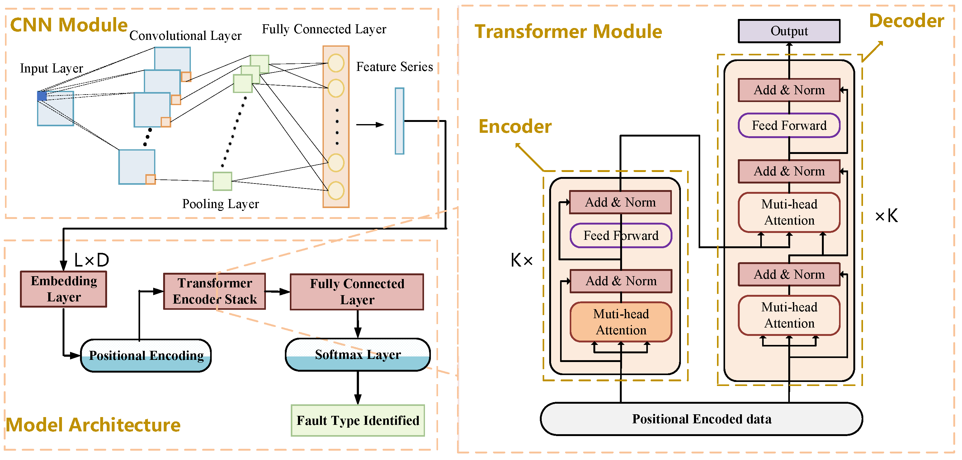
Considering both spatial and temporal dimensions to fully explore fault characteristics, this paper constructs a multi-input and single-output CNN-Transformer neural network model to learn the features under various operating conditions of optical CTs for fault identification; the details of model are shown in
Figure 2. What is more, the dataset is split for training, validation, and testing with a ratio of 7:1:2. The parameters in the model are optimally selected through grid search algorithm. By traversing various combinations of optional parameters of the model, we select the set of model parameters with the best identification performance on validation dataset as the model parameters. The optional values of parameters are shown in
Table 1.
To begin with model construction, the data processes like data cleaning and data normalization are performed, and each parameter of every sample for optical CT is in the range [0, 1]. Furthermore, due to there being six operating states of optical CT states in total, the identification results include 0~5, with 1~5 representing five fault types and 0 representing normal operating state.
Given that the occurrence of a single fault in an optical CT often accompanies changes in multiple state parameters, and changes in one parameter can potentially lead to various faults, it means that the different components of optical CT will interact with each other, indicating that there exists a complex spatial interrelationship in this device. The Convolutional Neural Networks (CNNs) [
22,
23,
24], which mainly consist of the following structures, input layer, convolutional layer, pooling layer, activation layer, and fully connected layer, are employed in this context. The convolutional layer is primarily tasked with extracting features from input data. In this process, the convolutional kernels (or filters) slide over the data series, performing element-wise multiplications and summing the results to generate features. The resulting feature data often contain a substantial number of pixels; hence, a down-sampling operation known as pooling technique is used to make feature selections, further enhancing the efficiency and generalization ability of feature extraction and making CNNs highly effective at learning internal relationships related to optical CT faults.
The dimension of data series defined in this study is 96 × 5, meaning the time sequence concludes the operating data of 96 timesteps before and at the time of identification, and each data concludes 5 features. And the convolutional kernels with dimensions of 2 × 2 and the max pooling strategy to undergo feature extraction. After that, the dimension of features series is 94 × 1. The calculation of feature extraction is as follows:
where
is the weight of the
k-th convolution kernel. Bias
representing convolution operations;
is used to activate the function.
The Transformer model [
25], proposed by Google in 2017, is famous for its ability to exact features in temporal dimension. One of its key advantages is the self-attention mechanism, which allows the model to consider all information in time series simultaneously, enabling it to capture complex relationships effectively, even over long distances. This feature significantly enhances the model’s ability to extract valuable information within data. Furthermore, positional encoding ensures that the model retains information about the order of tokens in a sequence. By adding positional encodings to the embedding layer, Transformers can understand relative positions between sequences, which is crucial for maintaining the integrity of series structures. Last but not least, the multi-head attention mechanism further boosts the model’s expressiveness by allowing it to focus on different parts of the input simultaneously. Each attention head captures distinct features from various subspaces, providing a richer representation of the input data. It is believed that this model can contribute greatly to fault identification.
In detail, this model mainly consists of two structures, encoder and decoder, as shown in
Figure 2. The left and right sides correspond to the encoder and decoder structures, respectively. Both are composed of several basic Transformer blocks, which comprise a multi-head self-attention (MSA) block, a feedforward neural network (FNN), and layer normalization (represented by the light-colored boxes in the figure). Specifically, the input dimension of the first encoder in the encoder stack is L × D, where L is the length of input data dimension, set as 94 in this study, and D is a hyperparameter representing the embedding output dimension, set as 12 in this study. Due to the existence of the muti-attention head, the input is split into K which is the number of attention heads, set as 3. The dimension of input of each encoder is L × (D/K), namely 94 × 4 in this study.
Before the feature sequence
after CNN module is sent to Transformer structure, the embedding layers and positional encoding layer are used to preprocess:
where
is the multiplication parameter that needs to be trained for the embedding layers.
is the dimension of the time series,
denotes the
i-th dimension of vector,
is the exact position of the current feature. Through this data preprocessing, the model can better capture the correlation between optical CT features at different time periods.
After that, the input
is linearly transformed into a query matrix
, a key matrix
, and a value matrix
. The attention weights are obtained by computing the dot product of
and
, followed by scaling and a softmax operation, as expressed by
where
is the dimension of
. To capture information from different subspaces,
,
, and
are usually split into multiple heads, with each head calculating attention scores in parallel. The outputs of these heads are concatenated and linearly transformed to obtain the MSA score, expressed as
where
is the number of heads and
is the weight matrix of the linear transformation. The output of the
i-th head can be calculated by the following formula:
where
,
, and
represent the weight matrices of the query, key, and value of the
i-th head, respectively.
Then, the feature is sent to fully connected feedforward network, which consists of two dense layers, and the Relu-activated function is adopted for non-linear transformations.
where
and
are the linear transformation parameters,
and
are the bias vector,
denotes the Relu activated function.
After the feature is obtained based on Transformer model, it is sent to fully connected layer, with its dimension transforming from 94 × 4 into 94 × 6, for the reason that there are 6 operating states of optical CT. Finally, based on the softmax layer, the identification result can be generated.
Overall, for the identification of state of optical CT in timestamp , the CNN module is used for spatial feature extraction while the Transformer module is constructed for temporal feature extraction, depending on which the accurate identification results will be obtained.
2.2. Fault Severity Assessment
This fault severity assessment model is mainly based on the idea that the more different the state of optical CT from the normal state, the more severe the fault will be, which is testified shown in part III. In this study, the method of Shapley Additive Explanations (SHAP) is used to quantify the importance of each parameter in optical CT during different faults. Also, the range of parameters of optical CT in different operating states will be concluded according to the results of scene generation in next part, based on which the assessment of fault severity will finally be obtained.
SHAP constitutes a model interpretation framework grounded in cooperative game theory [
26,
27]. This approach primarily leverages the Shapley value, an element from cooperative game theory that gauges how much each team member contributes to the collective gain. In this context, the Shapley value is employed to measure both the extent and direction of influence that input features have on fault identification outcomes, as illustrated below. The absolute value of the Shapley value signifies the degree of contribution of each feature towards the identification results; the larger the absolute value, the more significant the contribution. Furthermore, the impact direction of these features on identification outcomes is denoted by whether their Shapley values are positive or negative.
where
is the Shapley value of feature
, which is the
n-th input features.
is the complete set of all the input features while
is a subset of
. The condition
means that
can only be a subset of
that does not include feature
,
is the output when the feature subset
is input,
is the output when the feature subset
plus feature
as input, then
can represent the marginal contribution of feature
. From the equation, it can be concluded that SHAP creates various subsets
of feature combinations, assessing the impact of including or excluding each feature
on the model’s output.
Considering the fact that under different fault states, the optical CT will show completely different operating characteristics, meaning that the importance of features of optical CT will vary with operation state. So, for every fault type, the binary identification model is constructed based on CNN-Transformer model with its results belonging to this type or not. Then, the SHAP algorithm is adopted for binary identification model to evaluate the importance of features under this operating state, referred to as , , …, . After that, based on the upper and lower bounds of normal operating state of optical CT, the assessment can be obtained.
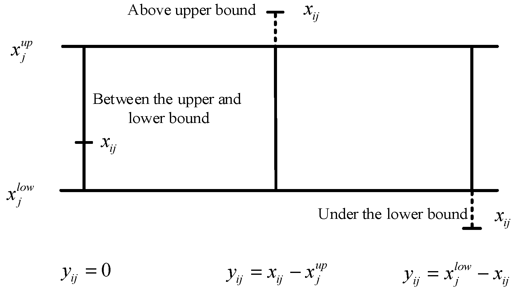
The comprehensive evaluation indicators
is
where
and
are the upper and lower bounds of the
j-th feature of normal operating states, respectively, which is obtained according to “SCENE GENERATION” part.
is the number of total features,
is the difference between normal state and fault state for
j-th feature.
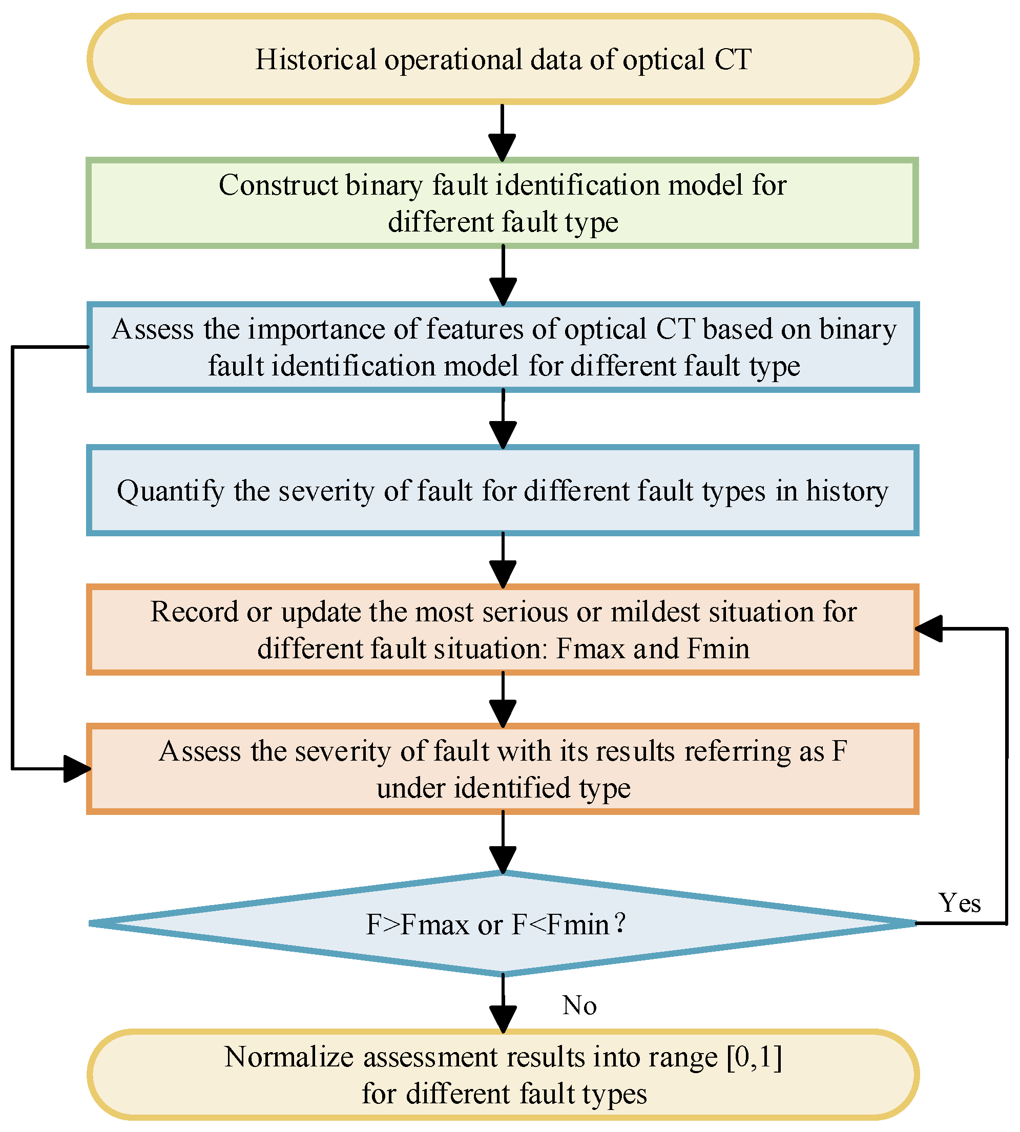
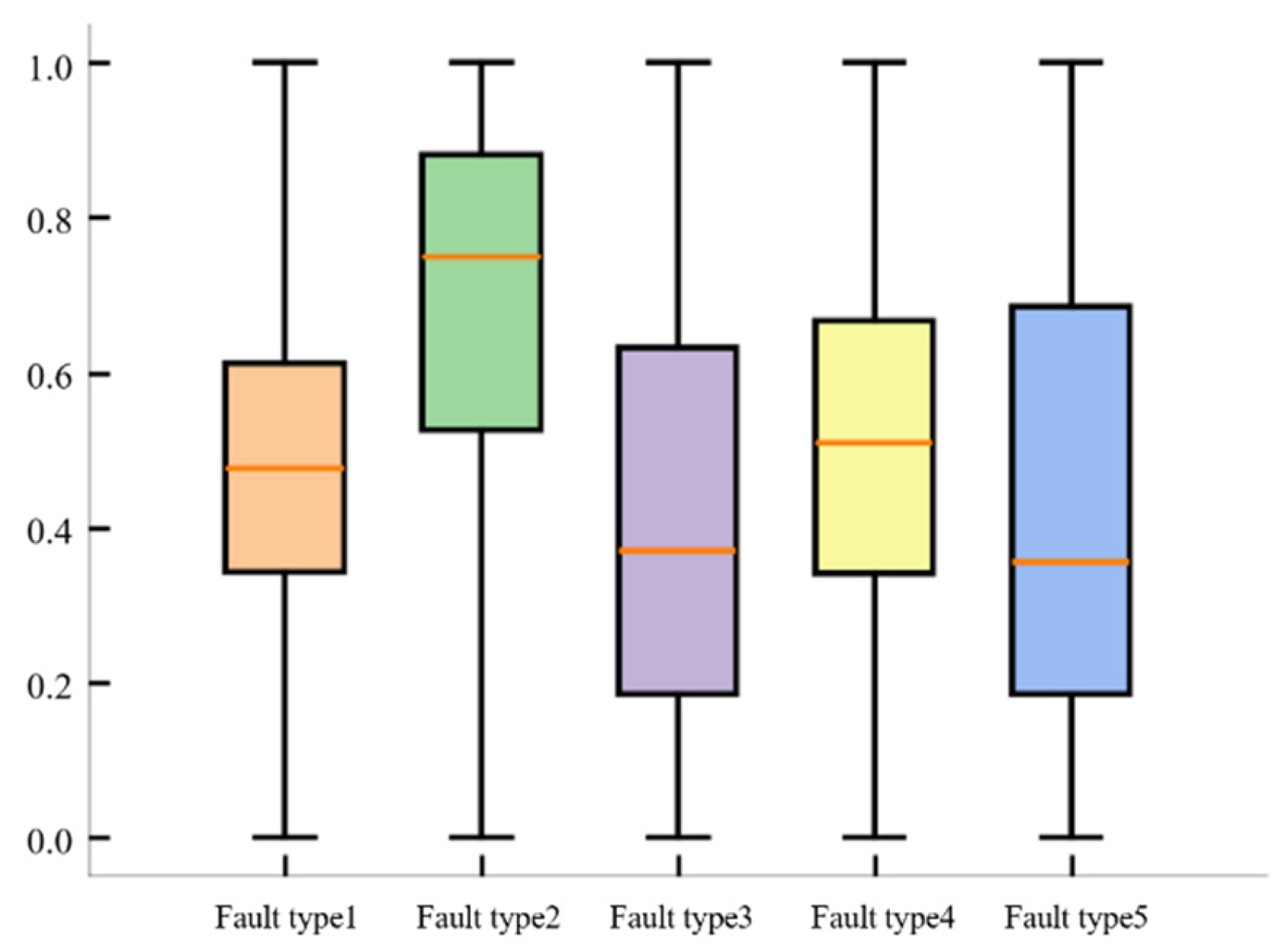
It can be seen from
Figure 3 that when the optical CT is operating normally, the comprehensive evaluation index is equal to zero. The larger the fault, the more severe the fault. For each fault situation, calculate the comprehensive evaluation indicators for the most severe fault situation
and the least severe fault situation
in the history of the fault. Quantify the severity of each future sample’s corresponding fault type based on fault identification and normalization:
It can be seen that
is in the range of [0, 1], and the closer it is to 1, the more severe the fault is. When a fault that is more severe or less severe than the historical situation occurs in the future, it is necessary to update
and
in real-time. The algorithm flowchart is shown in
Figure 4.
2.3. Scene Generation
This study evaluates the severity of faults by analyzing the degree of difference between optical CT fault conditions and normal conditions. However, due to the limited historical samples, it is impossible to accurately conclude the exact upper and lower bounds of various parameters under different operating conditions of optical CT. Therefore, this study first used the k-means-SMOTE algorithm to simulate and generate a large number of virtual samples and analyzed them to improve the robustness of severity assessment.
Considering that the SMOTE models rely on the sample distribution characteristics, they will suffer from overfitting and difficulties in effectively processing datasets with uneven sample spacing, which will lead to poorly generated data. Due to the low occurrence frequency and sparse data sample space of fault samples, the k-means-SMOTE algorithm first uses the k-means clustering algorithm to cluster the specific operating type of sample into several clusters and then applies SMOTE within each cluster to improve the reliability of sample generation. In this way, the data will be generated from the data clusters with much tighter sample space, which will be more similar to the distribution of real data. The following contents introduce the method for a certain type of fault as an example.
At first,
cluster centers
are randomly selected from samples under the same fault type, and the historical dataset is divided into clusters according to the k-means clustering algorithm [
28]:
where
means the type of cluster division, while
means the possible type of cluster the sample
might belong to.
denotes the possible cluster center the sample
might belong to. The sample belonging to
means the cluster is more similar to the cluster center
than other cluster centers. This algorithm iteratively adjusts the cluster centers to minimize the Euclidean distance
between all samples and their corresponding cluster centers, achieving sample clustering.
Subsequently, based on the number of samples
in each cluster, the appropriate number of new synthesized samples
that need to be generated is determined. Each time a sample is generated, the SMOTE algorithm randomly selects a sample
, where
represents the
j-th operating parameter. Then, the
nearest neighbors to the sample based on the Euclidean distance are found, and one of the neighboring samples is randomly selected to generate samples using the following equation.
In the formula, is a randomly selected number from the interval [0, 1], which is used to control the distance between the new sample and the original sample. represents the generation of the j-th operating parameter, representing the simulated generated operating sample.
Finally, the identification model is used to identify fault types in the generated sample data. In the formula,
represents the identified fault label of generated sample
.
For each generated sample, fault identification is performed based on the CNN-Transformer model, and samples with the identified result of the same state as the generated type are selected for sample expansion. Further statistical analysis is conducted to determine the upper and lower bounds of each parameter under different operating states of optical CT in order to improve the robustness of the statistical results. For example, when it comes to normal operation state, the upper and lower bound, defined as
and
, can be obtained according to following equations:
where the
represents the set of the
j-th operating parameter of generation samples in normal operating state, while the
represents the set of the
j-th operating parameter of historical samples in normal operating state.


 and
and 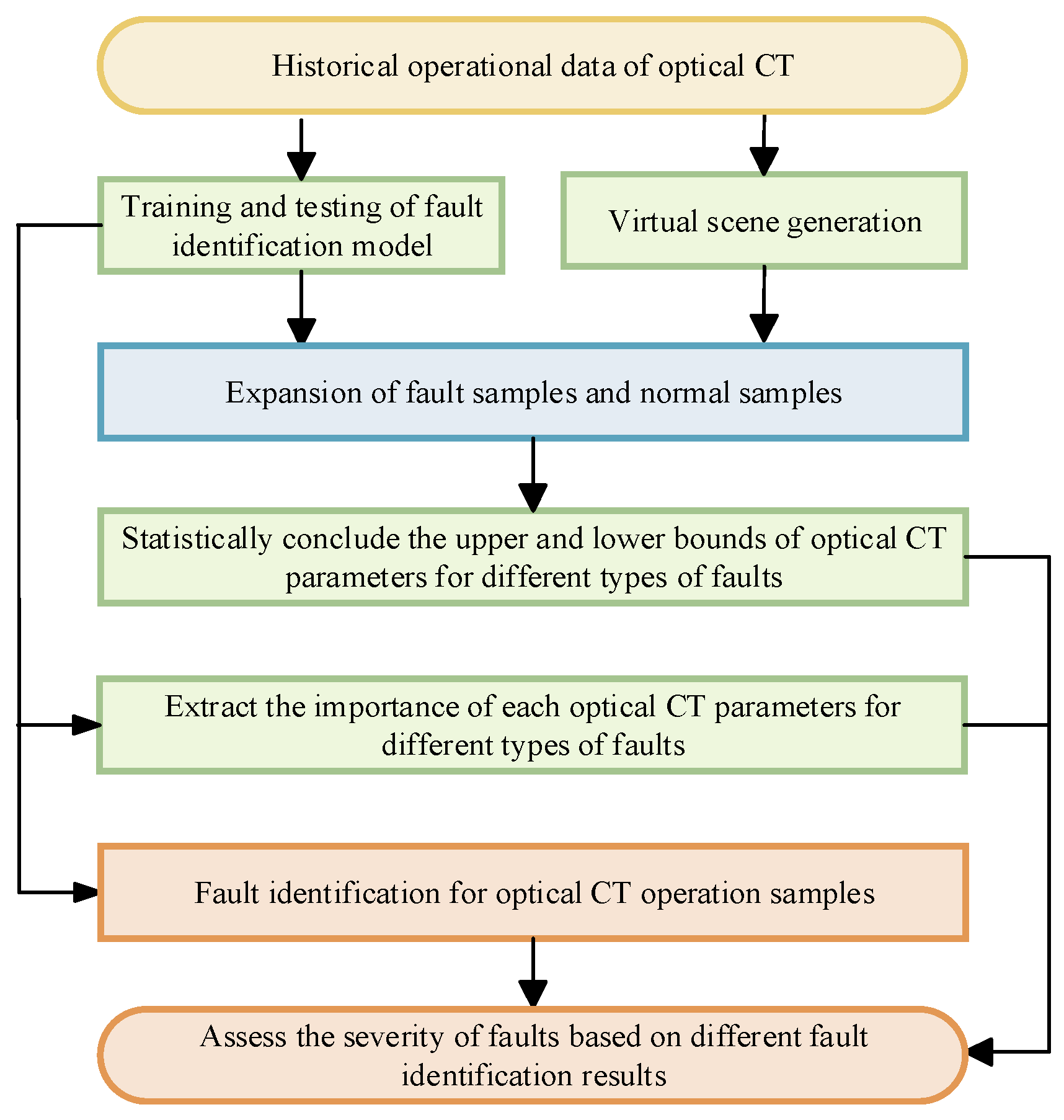
