Forecasting Ethanol and Gasoline Consumption in Brazil: Advanced Temporal Models for Sustainable Energy Management

Abstract

The sustainable management of energy resources is fundamental in addressing global environmental and economic challenges, particularly when considering biofuels such as ethanol and gasoline. This study evaluates advanced forecasting models to predict consumption trends for these fuels in Brazil. The models analyzed include ARIMA/SARIMA, Holt–Winters, ETS, TBATS, Facebook Prophet, Uber Orbit, N-BEATS, and TFT. By leveraging datasets spanning 72, 144, and 263 months, the study aims to assess the effectiveness of these models in capturing complex temporal consumption patterns. Uber Orbit exhibited the highest accuracy in forecasting ethanol consumption among the evaluated models, achieving a mean absolute percentage error (MAPE) of 6.77%. Meanwhile, the TBATS model demonstrated superior performance for gasoline consumption, with a MAPE of 3.22%. Our models have achieved more accurate predictions than other compared works, suggesting ethanol demand is more dynamic and underlining the potential of advanced time–series models to enhance the precision of energy consumption forecasts. This study contributes to more effective resource planning by improving predictive accuracy, enabling data-driven policy making, optimizing resource allocation, and advancing sustainable energy management practices. These results support Brazil’s energy sector and provide a framework for sustainable decision making that could be applied globally.

1. Introduction

One of the most pressing global challenges today is ensuring the sustainable supply of clean energy for future generations, especially in light of the environmental commitments established since the Kyoto Protocol. These commitments have created an urgent need to reduce greenhouse gas emissions and transition to cleaner energy systems, spurring significant interest in renewable energy sources. Among these alternatives, biofuels stand out as a highly viable option, particularly for countries like Brazil, which possesses abundant natural resources conducive to renewable energy production. Renewable energy sources—such as solar, wind, hydropower, and biofuels—represent the cornerstone of global efforts to mitigate climate change and ensure energy security. Within this spectrum, biofuels are particularly promising due to their capacity to reduce dependence on fossil fuels, which continue to dominate Brazil’s energy matrix. These fuels are sustainable and capable of lowering carbon emissions, but they also have a significantly reduced environmental footprint compared to conventional energy sources. Additionally, renewable energy sources are derived from inexhaustible materials, such as sunlight, wind, water, and organic waste, which can be repurposed efficiently as by-products of other economic processes, as highlighted by [1,2,3].

A key characteristic of biofuels, such as ethanol, is their ability to support a circular economy. Biofuels are produced from agricultural residues or crops like sugarcane and corn, and their by-products can be reintegrated into various production cycles. This not only enhances resource efficiency but also reduces waste, a principle that aligns with the goals of sustainable development. For instance, sugarcane bagasse—a residue of ethanol production—is often used to generate electricity, adding another layer of sustainability to the biofuel value chain. Addressing environmental concerns cannot be overstated in discussions surrounding sustainable development. Burning petroleum-based fuels, which release significant quantities of carbon dioxide (CO₂) into the atmosphere, is a central driver of global warming. This process exacerbates the greenhouse effect, leading to climate-related challenges, including extreme heatwaves, rising sea levels, and increasingly erratic weather patterns [4]. Anthropogenic CO₂ emissions are particularly alarming, with global concentrations surpassing pre-industrial levels by 50%, as reported by the United Nations Framework Convention on Climate Change (2023). This sharp increase reached critical levels in 2022, contributing to severe and widespread climate disruptions. The associated socioeconomic and environmental consequences—such as biodiversity loss, water scarcity, and economic instability—demand urgent and coordinated global action [5,6].

As a renewable biofuel, ethanol offers a practical and environmentally friendly alternative to fossil fuels. Produced primarily from sugarcane in Brazil, ethanol has several environmental and economic advantages. Its combustion produces fewer harmful emissions, such as sulfur oxides (SO₂ and SO₃), which are responsible for acid rain [7]. Moreover, ethanol’s production process can be optimized to minimize costs and maximize efficiency, especially when integrated with advanced technologies. Despite its limitations, such as lower energy density than gasoline and the potential environmental impact of large-scale agricultural cultivation, ethanol remains a cornerstone of Brazil’s energy policy due to its sustainability and potential for economic scalability [3,8].

Given the potential for economic scalability, the analysis of Brazilian ethanol consumption can be effectively explained as a function of time through time–series modeling. This approach provides a structured framework to understand temporal behavioral patterns and describe the underlying phenomena. The versatility of forecasting models spans numerous fields of study, primarily due to the temporal dependencies inherent in most variables. Among the most established classes of time–series models is the methodology proposed by Box and Jenkins [9]. Their approach decomposes time–series data into autoregressive and moving average components, enabling the detailed analysis of trends, correlations, and overall behavior within the observed data. Such analyses generate viable and reliable estimates of the phenomenon under study [2].

Contributions and Limitations

The primary contribution of this research lies in the comparative analysis of the forecasting performance of various univariate time–series models, including ARIMA/SARIMA, Holt–Winters, ETS, TBATS, Facebook Prophet, Uber Orbit, N-BEATS, and TFT. By evaluating the strengths and limitations of each methodology, the study identifies the most accurate models for estimating ethanol and gasoline consumption in Brazil. A critical focus is placed on achieving a mean absolute percentage error (MAPE) of less than 10%, a high-precision forecasting benchmark. These models were subsequently applied to project sales volumes through 2030, thereby contributing to evaluating compliance with the Sustainable Development Goals (SDGs) that are related to biofuel consumption in a country endowed with abundant green energy resources, such as Brazil.

In addition to fostering an understanding of trends in sustainable energy consumption, the results contribute to policy decisions and strategic planning in the renewable energy sector, reinforcing Brazil’s role as a global leader in renewable energy development. However, the study presents limitations, such as the exclusion of exogenous variables, such as economic indices, and other biofuels, like biodiesel. Including such variables as economic indicators or policy changes related to biofuels can significantly improve forecasting accuracy by reflecting real-world conditions. These factors allow the model to account for external shocks impacting biofuel production and demand. However, incorporating such variables requires prior analysis, such as studying the causality between exogenous and endogenous variables [2], which is beyond the scope of this work.

Structurally, the paper includes a literature review on biofuels in the context of energy management, public policies, and international sustainability goals, followed by a detailed methodology, statistical analysis of time–series patterns, and a comparison of model accuracy. The conclusion summarizes the main findings, discusses practical implications, and proposes directions for future research, offering a clear and comprehensive roadmap that connects theoretical foundations to practical applications, contributing to advancing research on biofuels and energy transitions.

2. Literature Review

Accurately forecasting biofuel consumption is crucial in optimizing the allocation and sustainable management of natural resources for energy generation. This process enhances operational efficiency within the biofuel industry and supports global efforts to transition to more sustainable energy practices. By aligning resource utilization with projected consumption patterns, forecasting reduces waste, improves supply chain management, and ensures energy security. Furthermore, it significantly advances the United Nations’ Sustainable Development Goals (SDGs), particularly SDG 7 and SDG 12, which are directly related to energy access, renewable energy, and sustainable resource management [2,3].

In this way, SDG 7 aims to ensure global access to modern, reliable, and affordable energy services (SDG 7.1), increase the share of renewable energy in the global energy mix (SDG 7.2), double the global rate of energy efficiency improvements (SDG 7.3), and strengthen infrastructure for sustainable energy services in developing countries (SDG 7.5). Meanwhile, SDG 12 focuses on promoting sustainable management and efficient use of natural resources (SDG 12.2), raising awareness about sustainable development (SDG 12.8), strengthening the scientific and technological capacities of developing countries (SDG 12.A), and eliminating inefficient fossil fuel subsidies (SDG 12.C). Accurate energy consumption forecasts are essential for making informed decisions that align with these objectives, considering both long-term factors, such as socioeconomic changes and technological advancements, and seasonal factors, such as weather variations and industrial activity cycles. These aspects are essential for integrating renewable sources (SDG 7.2) and developing sustainable energy infrastructure (SDG 7.5) [2,10].

Furthermore, policymakers can make analytical decisions regarding energy and agricultural policies, leading to the implementation of regulations that promote sustainable production practices. It is also possible to minimize environmental impacts while improving agricultural productivity, emphasizing the need for sustainable farming practices. Enhancing efficiency in using resources, such as sugarcane and corn for ethanol production, can be achieved through targeted research and development based on consumption forecasts [11]. Unpredictable events, including economic fluctuations and changes in the political landscape, highlight the necessity of implementing sophisticated forecasting methodologies to foster international cooperation in clean energy research and technological advancements and strengthen developing countries’ scientific and technological capacities to achieve more sustainable consumption and production practices. By employing appropriate forecasting strategies, service providers and researchers can contribute to initiatives aimed at expanding access to clean energy, constructing sustainable renewable energy infrastructures, and advancing objectives focused on optimizing the inefficient use of fossil fuels.

Regarding the sustainability of biofuels, several key factors must be considered, including land use and food security. According to [12], accounting for variable demand can foster the synergistic development of agriculture, renewable biomass feedstock, and biofuels. Fuel production has the potential to sustainably utilize marginal lands and agricultural residues without directly competing with food crops. Furthermore, biofuels represent a viable alternative to fossil fuels, contributing to the reduction in greenhouse gas emissions and the mitigation of ozone layer depletion [13,14]. To further reduce environmental impacts, strategic planning of agricultural expansion is essential [3,15].

As highlighted by [16], limiting agricultural expansion to regions with lower conservation importance could reduce carbon emissions from biofuel-related land use changes by up to 87% and decrease biodiversity impacts by 41%. Understanding biofuel consumption is fundamental for shaping public policies, encouraging sustainable production practices, and stimulating the biofuel market. Moreover, accurate knowledge of biofuel consumption allows cities to plan and implement strategic energy management, develop energy policies, promote rural and agricultural development, and drive technological advancements [17]. Analyzing usage trends enables authorities to identify periods of high demand, optimize resource allocation, and implement demand response strategies, thereby reducing dependence on fossil fuels and fostering sustainable urban development initiatives [18]. This approach is not limited to urban contexts but can also be applied across other sectors, improving fuel efficiency and lowering operational costs [2,3,15,19].

The main types of biofuels produced in Brazil are ethanol and biodiesel, with ethanol taking a critical position due to its extensive production from sugarcane. This advantage in agriculture allows Brazil to be a leading player in the global ethanol market, offering a renewable energy source that significantly reduces carbon emissions. Ethanol has a noticeable role in the country’s energy strategy and is widely used in the flex-fuel vehicle fleet, which can run on varying blends of ethanol and gasoline. It has great potential to reduce Brazil’s reliance on fossil fuels, foster economic growth in rural areas, create jobs, and support the country’s environmental objectives.

Brazil’s ethanol production represented 30% of the global production of this fuel in 2020 [20]. However, demand for ethanol is expected to grow, driven by domestic consumption and market dynamics. Ref. [21] highlighted that, if biofuel producers fail to meet rising demand, it could adversely affect the economy and hinder the commitments made by the Brazilian government. The Energy Research Office (EPE) predicts a 5.1% increase in hydrous ethanol demand in 2024 and 3.8% in 2025. It should be noted that ethanol consumption is closely related to gasoline and hydrous ethanol prices. Therefore, the increase in gasoline prices in 2024, as reported by the Department of Information, Studies, and Energy Efficiency (DIEE), indirectly conveys that consumers are expected to shift towards ethanol, which is often more cost-effective.

Still, predicting and meeting future fuel and biofuel needs have become increasingly complex and challenging for planners and utility providers, particularly in developing countries like Brazil [22]. As the global population goes through growth, urbanization, and industrialization, the need for energy is escalating, leading to uncertainties in future consumption trends [23,24]. In particular, this has been a global concern considering the increasing popularity of electric vehicles (EVs) [25], possibly changing consumer preferences. Such factors could lead to a decline in gasoline usage, which may affect ethanol consumption.

Due to the relevance of the area, the consumption of biofuels in Brazil has been forecast using time–series models, which are also related to industrial development (see [2,3,19]). However, these models are either outdated [26] or do not compare results with fuel oil consumption, such as gasoline [27]. This study overcomes these limitations and provides updated forecasts for ethanol and gasoline consumption in Brazil through 2030, which align with the SDGs.

Table 1. Comparative study.

Ref.	Year	Region	Model	Fuel	MAPE (%)	Residuals
[29]	2018	Cameroon	MLR	Gasoline	7.651	✓
[30]	2020	China	EGM (1,1,$\alpha$,$\theta$)	Ethanol	4.314	✕
[30]	2020	India	EGM (1,1,$\alpha$,$\theta$)	Ethanol	3.621	✕
[30]	2020	USA	EGM (1,1,$\alpha$,$\theta$)	Ethanol	1.002	✕
[31]	2022	Turkey	RF	Gasoline	11.529	✕
[32]	2023	India	ARIMA (2,1,1)	Ethanol	3.871	✓
Current Paper	2024	Brazil	TBATS	Gasoline	3.22	✓
Current Paper	2024	Brazil	Orbit	Ethanol	6.77	✓

compares the best MAPE results of the current article with other articles on fuel demand forecasting. Despite some of them performing better, it is noticeable that the best results of different studies primarily do not evaluate the presence of autocorrelation within the residuals, such as with the Ljung–Box test, as expressed in the Residuals column of the table. This can significantly interfere with determining the most appropriate model and its respective MAPE. As evidenced by Table 1, our work has achieved the best MAPE value for gasoline consumption prediction, with both TBATS and Orbit achieving highly accurate results [28], whilst also checking for the presence of autocorrelation within the residuals. Our work also compares several forecasting models’ accuracy for Brazilian ethanol and gasoline consumption.

Predictive modeling has also been used in different domains. As examples, ref. [33] develops a lightweight deep learning model (CE-CNN) to predict NOx emissions in coal-fired boilers, improving accuracy and efficiency, whilst [34] explores time–series forecasting for financial profit analysis, comparing ARIMA, SARIMA, and LSTM, concluding that LSTM outperforms statistical models. These works evidence the effectiveness and contributions of advanced machine learning and time–series techniques in several fields.

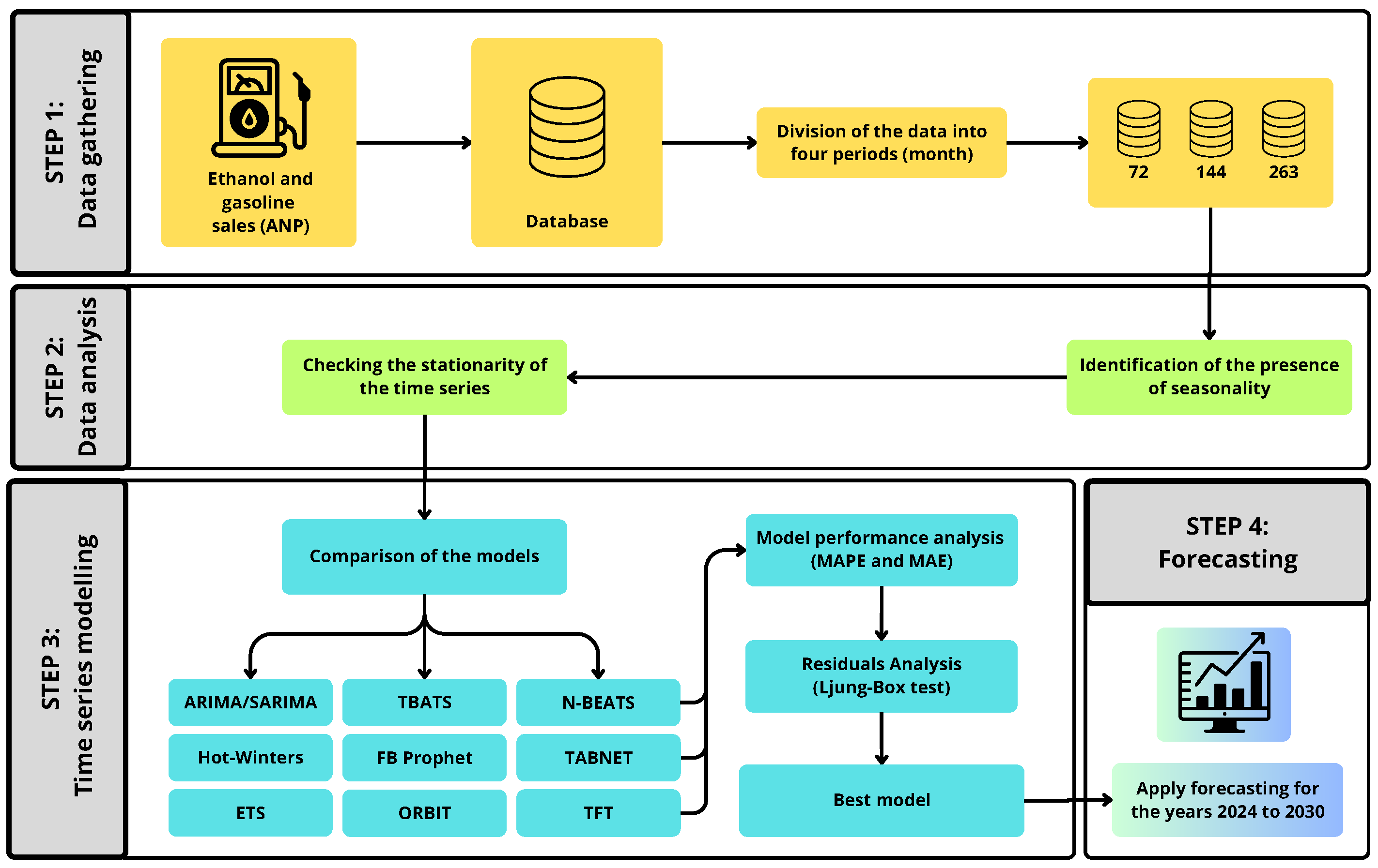
3. Methodology and Materials

The research methodology illustrated in Figure 1 is systematically divided into four distinct phases, each contributing to the overall forecasting process. The first phase, data preprocessing, involves cleaning, transforming, and preparing raw data for analysis. This step ensures data consistency by addressing missing values and outliers and standardizing datasets to enhance compatibility with the selected models. Key processes in this phase include data normalization, seasonal data composition, and exploratory data analysis, all of which help uncover underlying patterns and trends. In the second phase, model implementation, a diverse range of forecasting models is applied, from classical statistical methods to advanced machine learning algorithms and deep learning architectures.

The third phase, performance evaluation, assesses the predictive accuracy and robustness of the models using well-established metrics such as the mean absolute percentage error (MAPE), root mean square error (RMSE), and normalized RMSE. Additionally, the Ljung–Box test analyzes the presence of autocorrelation in the residuals. Finally, in the forecasting phase, the most accurate models identified in the evaluation phase are employed to predict future biofuel consumption trends. These forecasts support strategic decision making and inform policy development. This structured methodology ensures a rigorous and systematic approach to biofuel consumption forecasting, enhancing the reliability and applicability of the results.

This study focuses on a comparative analysis of advanced forecasting models’ accuracy in predicting Brazil’s biofuel demand. Its primary objective is to support the achievement of SDG 7 (Affordable and Clean Energy) and SDG 12 (Responsible Consumption and Production). By assessing the performance and robustness of these models, the research aims to identify methodological improvements that can enhance projections in the context of sustainable energy policy planning.

The predictive models investigated in this research utilize diverse methodologies, as illustrated in Figure 1. These include classical statistical models such as the Autoregressive Integrated Moving Average (ARIMA) and its seasonal adaptation (SARIMA), proposed by Box and Jenkins (1994) [9], and the Holt–Winters method described in [35]. Additionally, the study evaluates contemporary models, such as Facebook Prophet (FB Prophet) [36], Object-Oriented Bayesian Time–Series (Orbit), and Neural Basis Expansion Analysis for Time–Series Forecasting (N-BEATS) [37]; additionally, Time Fusion Brazil’s expected ethanol and gasoline sales volumes include the Box–Cox Transformation approach, combined with ARMA Errors, Trends, and Seasonal Components (TBATS) [38], and Exponential Smoothing (ETS) [39].

The selected models encompass a diverse range of forecasting approaches, including classical statistical models (ARIMA, SARIMA, Holt–Winters, ETS, TBATS), hybrid statistical–machine learning models (Facebook Prophet, Uber Orbit), and deep learning architectures (N-BEATS, TFT). This selection compared well-established, interpretable models with more complex, data-driven methods, ensuring a comprehensive evaluation of ethanol and gasoline consumption forecasting performance.

Each model represents a unique theoretical framework and approach to time–series forecasting, ranging from classical statistical methods to machine learning algorithms and deep learning architectures. The research also examines computational efficiency, scalability, and the suitability of these models for handling large-scale time–series data with seasonal and non-seasonal patterns.

Finally, the best-performing models with optimized configurations are employed to project future biofuel consumption trends in Brazil. These projections, extending through 2030, provide a detailed view of the expected ethanol and gasoline sales volumes, offering knowledge for strategic decision making and public policy formulation. Additionally, these forecasts align with the Sustainable Development Goals (SDGs), reinforcing their relevance within the context of energy transition.

Among the models utilized, ARIMA (Autoregressive Integrated Moving Average) stands out due to its widespread application in time–series analysis, particularly its ability to capture patterns and dependencies in data. However, complementary models have also been employed to ensure more robust and accurate forecasts, each exploring different aspects of time–series dynamics [2,3].

The Holt–Winters model, for instance, is a classical approach that utilizes additive or multiplicative components to model constant seasonality and trends. It is particularly effective for datasets exhibiting regular patterns over time. Meanwhile, the Prophet model, developed by Facebook, is widely recognized for its flexibility and ease of use. It combines robust modeling of trends and seasonality with the inclusion of external effects, such as holidays and specific events, making it ideal for time–series with predictable variations and well-defined behaviors.

On the other hand, the TBATS model is designed to handle more complex time–series, particularly those with multiple seasonalities or irregular patterns. It has been proven to be highly effective when seasonal cycles are not immediately noticeable. Deep-learning-based models, such as N-BEATS and TFT (Temporal Fusion Transformer), also introduce innovative approaches to time–series forecasting. The N-BEATS model leverages neural networks to identify nonlinear and dynamic patterns in data. In contrast, the TFT model employs attention mechanisms to integrate external variables into multivariate time–series, enabling more comprehensive and context-aware forecasts.

Combining these diverse approaches results in detailed and reliable forecasts, strengthening public policy formulation and strategic planning in the energy sector. Thus, this study’s findings contribute to more assertive decision making and enrich Brazil’s sustainable energy transition, ensuring more efficient planning aligned with the country’s future needs.

3.1. The Dataset

This section provides information about Step 1, as shown in Figure 1. The data used in the models for this study were obtained from the Brazilian National Agency for Petroleum, Natural Gas, and Biofuels (ANP). They refer to the sales volume in liters for gasoline and hydrated ethanol from July 2001 to May 2024. For improved reproducibility, the dataset is published in a public repository (https://figshare.com/articles/dataset/Time_series_of_ethanol_and_gasoline_from_July_2001_to_May_2024_/26505391?file=48310720, accessed on 16 March 2025).

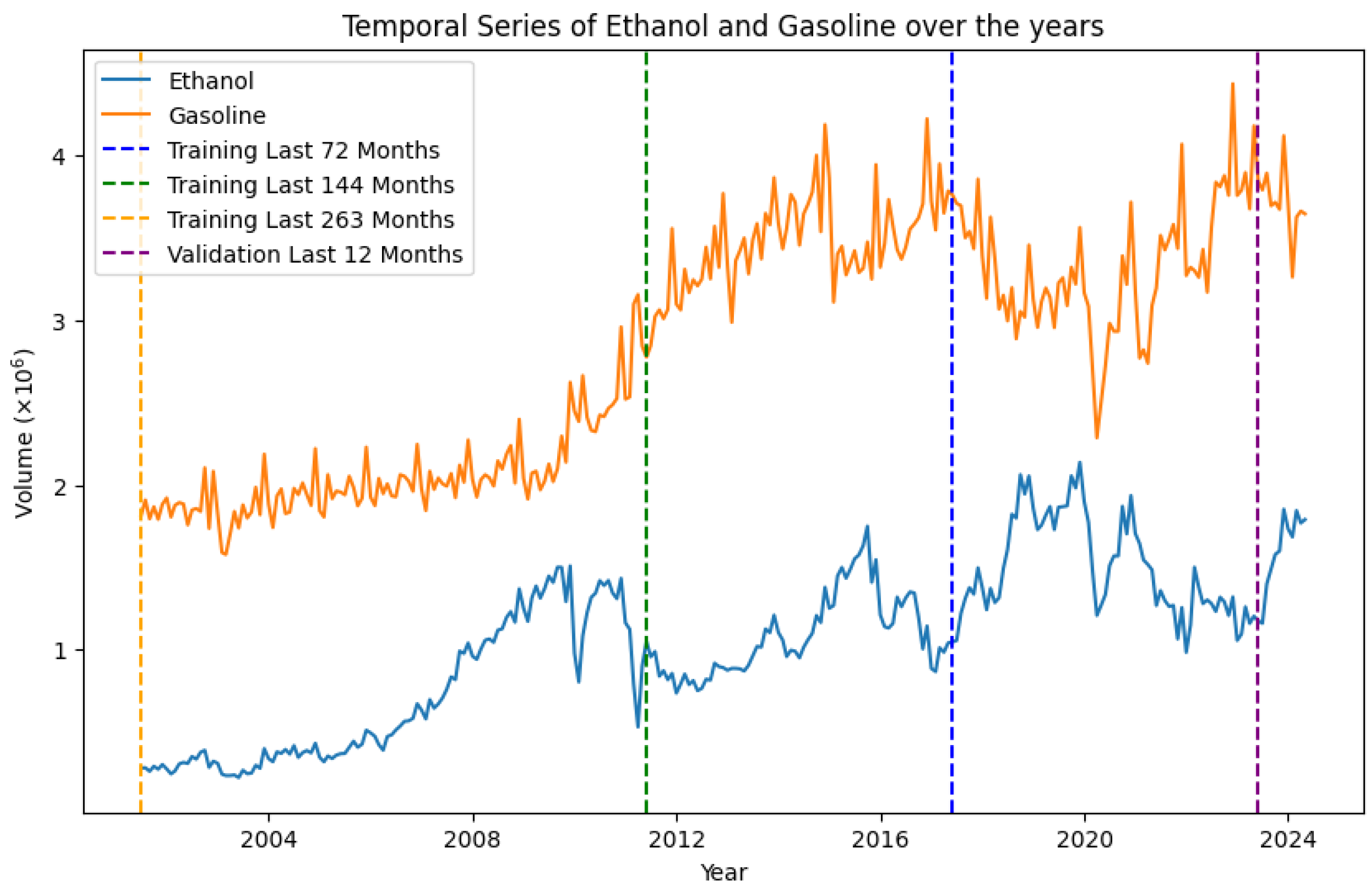
We opted for a customized data division approach instead of the standard 80:20 train/test split to better align with our analysis objectives. Specifically, instead of using the 80:20 ratio (which would yield approximately 230 training and 58 testing observations), our dataset, consisting of 275 months, was divided by reserving the last 12 months solely for testing—one year—while utilizing 263 months for training. This setup enables us to evaluate various training window lengths: 72, 144, and 263 months, along with 6 years, 12 years, and the entire dataset. Each duration targets different aspects, from recent trends to the complete historical range.

By structuring the data this way, we aim to capture a range of temporal patterns, particularly recent trends, that could enhance predictive power—something an 80:20 split might not effectively accomplish. This tailored approach provides flexibility in assessing how training length influences forecast accuracy.

Table 2. Summary of different training window lengths.

Window Length	Description
72 months	Focuses on recent data, emphasizing current trends for short-term forecasting.
144 months	Balances between capturing long-term trends and recent fluctuations, providing a broader historical context.
263 months	Uses the entire available dataset before the test period, leveraging all past information to identify long-term patterns and cyclical behavior.

best illustrates these three distinct time windows. By training models across these three varied windows, we analyze the impact of training length on model accuracy, determining whether recent data alone or a comprehensive historical context can yield better predictions.

This division strategy seeks to identify which training window most effectively captures the characteristics of the time–series, with Figure 2 offering a visual overview of the training window configurations. By training models across these three different windows, we analyze the effect of training length on model accuracy, determining whether recent data alone or a complete historical context results in better predictions. This division strategy seeks to identify which training window most effectively captures the characteristics of the time–series, with Figure 2 offering a visual overview of the training window configurations.

In Figure 2, note that each vertical dotted line marks a point for collecting training data up to the validation data marking line. Furthermore, the visual patterns in the gasoline data are more consistent, while the ethanol data seem to show more erratic patterns. The data spanning 263 months reflect a more significant behavior change compared to the more recent training periods. Ethanol is often promoted as a substitute for gasoline, yet the time–series data do not support this claim.

3.2. Model Evaluation and Forecasting

This subsection details the metrics and the Ljung–Box test used to assess the performance of the models presented in Step 3 of Figure 1. After the training phase, it is essential to conduct several tests for evaluation purposes to ensure accurate predictions on previously unseen data. Consequently, the model’s assessment is carried out by fine-tuning hyperparameters and analyzing performance metrics, such as the mean absolute percentage error ($MAPE$), the mean absolute error ($MAE$), the mean squared error ($MSE$), and the normalized root mean square error, based on the range between the minimum and maximum values ($NSRMS{E}_{minmax}$). These metrics are critical for determining the model’s effectiveness and precision in generating reliable predictions. Furthermore, the evaluation process may involve cross-validation techniques and sensitivity analysis to ensure robustness against different data variations. By employing these methodologies, the model’s capacity to generalize to new data is thoroughly tested, thereby enhancing the reliability of the forecasting outcomes.

The mean absolute percentage error ($MAPE$) measures the average percentage difference between the predicted and actual values, assessing the average magnitude of the model’s error. According to [28], $MAPE$ can be classified into different levels of accuracy, as shown in

Table 3. Forecast accuracy classification based on MAPE [28].

MAPE (%)	Evaluation
<10%	High accuracy
10% < MAPE < 20%	Good forecast
20% < MAPE < 50%	Reasonable forecast
>50%	Inaccurate forecast

.

The root mean squared error ($RMSE$) assesses the expected errors in projections, penalizing more significant deviations more heavily. This feature makes $RMSE$ a metric for identifying errors that deviate from expected behavior. Complementarily, the normalized root mean squared error ($NRMS{E}_{minmax}$) is an adjusted version of the $RMSE$, which considers the data variation, providing a more balanced view of the forecast quality in different contexts. The Ljung–Box test was used to verify whether the model correctly captured the structure of the analyzed time–series. This technique examines the residuals generated by the model, allowing the evaluation of errors. If the residuals do not exhibit autocorrelation, it is safe to affirm that the model achieved a good fit, indicating that the time–series structure was well understood.

To better capture dependencies in the data, training was performed with different window sizes and scenarios, such as biofuel consumption in Brazil up to 2030. This approach seeks to improve the precision and adequacy of the models by adapting them to different situations. Additionally, a comparison was conducted to verify the robustness of the models concerning biofuel trends. These tests considered the forecast precision, the computational speed, and the impact of external factors that may influence the analysis during the evaluated period. Consequently, the results are more likely applicable and reliable in real-world scenarios.

4. Time–Series Analysis

This section presents the results of statistical tests that assess features of the ethanol and gasoline time–series, as seen in Step 2 of Figure 1.

4.1. Seasonality Identification and Decomposition

Seasonality is a key feature in time–series modeling, as it helps distinguish cyclical behaviors from other components, such as trends and noise. Its identification is particularly relevant for models that require this attribute, such as Uber Orbit. The Autocorrelation Function (ACF) was used to detect seasonal patterns, with the results shown in Figure 3a,b for the ethanol and gasoline time–series, respectively.

The Autocorrelation Function (ACF) plots highlight a 12-month periodicity pattern in both time–series, as evidenced by the repetition of positive correlation peaks at regular intervals. This behavior indicates the presence of consistent annual cycles attributable to predictable seasonal factors. Among these factors are variations in fuel consumption associated with specific weather conditions during seasons, increased travel during holidays, and other annual events that directly impact supply and demand in the fuel sector. Identifying this periodicity is essential for time–series modeling, as seasonality is relevant in forecast accuracy and formulating policies and market strategies.

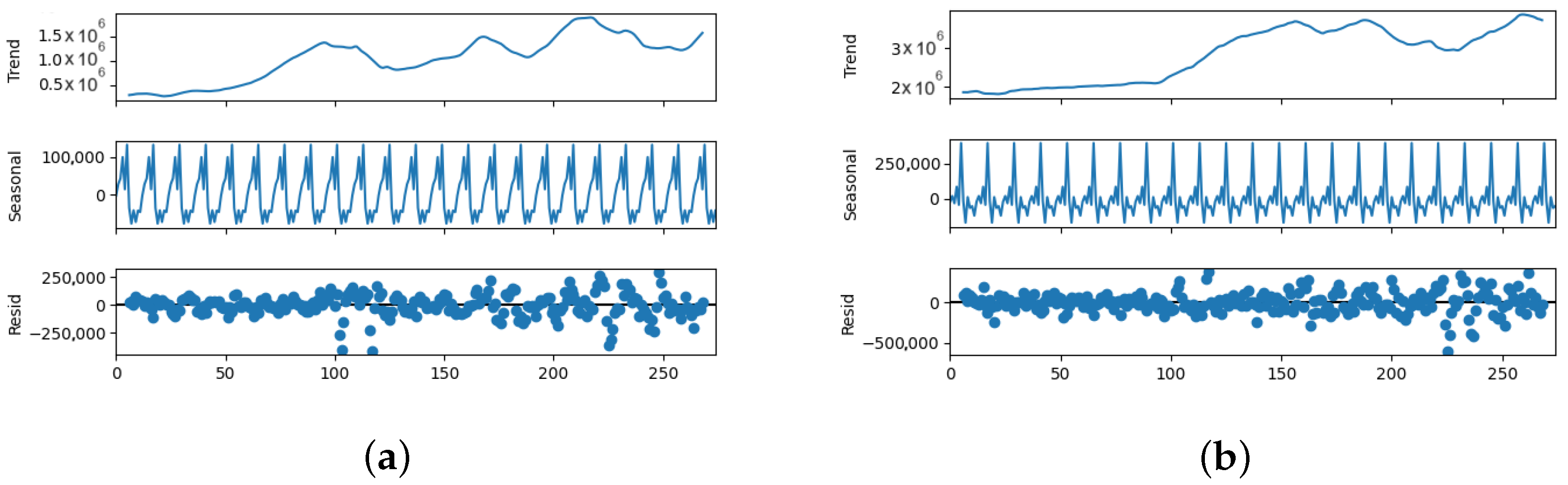
Based on this identification of periodicity, the time–series were decomposed into three fundamental components: seasonality, trend, and residuals. Decomposition is an indispensable methodological tool for gaining a more detailed understanding of the underlying patterns in time–series. It provides a segmented and precise analysis of how different factors impact the data. The seasonal component captures recurring and regular variations throughout the year, reflecting cyclical patterns that can be anticipated and considered in future analyses. The trend component highlights the overall trajectory of the data over time, enabling the identification of structural changes in consumption, such as gradual increases due to market expansion or decreases associated with economic or technological changes. Lastly, the residuals capture unexplained fluctuations not accounted for by the seasonal or trend components, representing deviations caused by unpredictable external factors, such as economic events, pricing policy changes, or extreme weather conditions.

The decomposition series into trend, seasonal, and residual components provides a robust framework for analyzing the behavior of ethanol and gasoline sales. By isolating these components, it is possible to identify and understand specific patterns that drive fuel consumption over time.

The seasonal component, illustrated in Figure 4a,b, reflects recurring patterns over 12 months. These cycles represent predictable annual fuel demand variations influenced by weather conditions, increased holiday travel, and other seasonal events. For instance, increased fuel consumption during the summer or holiday periods is evident in the consistent peaks presented in the seasonal plots. Recognizing these patterns is essential for short-term operational planning, such as efficient inventory management and resource allocation. By understanding these predictable cycles, businesses can optimize their supply chains and maintain efficient operations.

The trend component highlights the long-term direction of the data, revealing structural changes in the market. This component may indicate a steady rise in demand for ethanol due to the increased adoption of biofuels as part of renewable energy policies. In contrast, the trend in gasoline data may reflect fluctuations caused by economic growth, changes in vehicle ownership rates, or transitions to alternative energy sources. These results are fundamental for formulating long-term strategies, such as infrastructure investments or policy reforms, to adapt to market dynamics. The trend data supports future forecasting and enables stakeholders to anticipate and respond to macroeconomic and technological changes.

The residuals represent variations not explained by the seasonal or trend components. These irregularities often stem from unpredictable or one-off events, such as economic shocks, government policy changes, or supply chain disruptions. Analyzing residuals is essential for identifying uncertainties and preparing contingency plans, as they highlight deviations that cannot be anticipated through regular patterns. This analysis emphasizes the importance of flexible strategies, enabling businesses and policymakers to mitigate risks associated with unforeseen disruptions.

The combined analysis of ACF and decomposition provides a comprehensive and segmented understanding of the data, while the ACF confirms the existence of a 12-month periodicity; reinforcing the presence of seasonal cycles, the decomposition separates these cycles along with trend and residual components. This integrated approach allows for a more refined interpretation of fuel consumption factors.

Leveraging this knowledge, stakeholders can make better-informed decisions. For example, companies can align fuel distribution and supply chains with seasonal peaks and troughs, ensuring optimal operational efficiency. Policymakers can use trend data to anticipate long-term market changes and develop incentives for renewable energy adoption. Additionally, businesses can analyze residual patterns to prepare for potential disruptions, incorporating flexibility into their strategies to handle uncertainties effectively. Figure 4a,b visually represent these components, providing stakeholders with a clear depiction of the differences between ethanol and gasoline time–series. The distinction between seasonal, trend, and residual components enhances interpretability and supports data-driven decision-making processes.

In conclusion, this analysis enhances our understanding of time–series behavior. Dissecting and interpreting these components is vital for promoting sustainability and efficiency in the energy sector, which aligns with the broader goals of environmental responsibility and economic growth. This robust framework ensures that short-term and long-term strategies are well-informed and adaptable to changing market dynamics.

4.2. Stationarity Test

As seen from the time–series decomposition, a trend component is present from Section 4.1. This component demonstrated a growing trend in both series, suggesting they are not stationary. Many time–series models require stationarity for adequate forecasting; therefore, the number of differentiations necessary to achieve this feature must be estimated. To evaluate that, the Hylleberg, Engle, Granger, and Yoo (HEGY) test is applied [40]. This test examines the stationarity of time–series data by considering both deterministic components, such as seasonal effects and trends, and the presence of unit roots. The test returns p-values for different lag structures, with a p-value less than 0.05 indicating that the series is stationary and a p-value greater than or equal to 0.05 suggesting that the series contains unit roots. The HEGY test is useful for analyzing stationarity in time–series with a seasonal component, such as the ones in the scope of this work.

The test provides p-values for different components. The $t\_1$ statistic tests for the presence of a unit root at the non-seasonal frequency. The $t\_2$ statistic tests for unit roots at annual frequency. The p-values for these components are depicted in

Table 4. HEGY p-values for t_1 and t_2 for ethanol and gasoline time–series.

Time–Series	t_1	t_2
Ethanol	0.329	<0.001
Gasoline	0.793	<0.001
Ethanol Diff	<0.001	<0.001
Gasoline Diff	<0.001	<0.001

, which shows that, for the ethanol and gasoline time–series, the p-value for $t\_1$ is greater than 0.05, indicating that they are non-stationary at the non-seasonal frequency. In contrast, the p-values for $t\_2$ are all less than 0.001, suggesting that the series exhibits significant seasonal stationarity.

For the differenced series of ethanol and gasoline, both $t\_1$ and $t\_2$ show p-values less than 0.001, supporting the conclusion that differencing has rendered the series stationary regarding trend and seasonal components.

5. Results and Discussion

This section provides a comparative analysis of the models and applies the forecast generated by the best-performing model to each respective time–series. The comparison evaluates the model’s accuracy, efficiency, and overall performance across various metrics, enabling the selection of the most suitable forecasting approach for each dataset. The study aims to achieve optimal predictions tailored to each time–series’ unique characteristics by implementing the top-performing model.

5.1. Models Comparison

This subsection presents the results of the accuracy metrics and the analysis of the presence of autocorrelation in the residuals of the forecasting models, as shown in Step 3 of Figure 1. Since different models capture distinct aspects of the data and no single model is universally optimal for all datasets, this analysis aims to compare the accuracy metrics and residual autocorrelation of the selected models. This comparison aims to identify the model that best fits the characteristics of ethanol and gasoline sales volumes in Brazil. Considering the four different dataset sizes, the evaluation metrics results for each model are presented in

Table 5. Models comparison of MAE, RMSE, MAPE, and Ljung–Box with different input sizes.

Model	Fuel Type	Input Size
		72				144				263
		MAE ${\mathbf{10}}^{\mathbf{5}}\mathit{L}$	RMSE ${\mathbf{10}}^{\mathbf{5}}\mathit{L}$	MAPE %	Ljung -Box	MAE ${\mathbf{10}}^{\mathbf{5}}\mathit{L}$	RMSE ${\mathbf{10}}^{\mathbf{5}}\mathit{L}$	MAPE %	Ljung -Box	MAE ${\mathbf{10}}^{\mathbf{5}}\mathit{L}$	RMSE ${\mathbf{10}}^{\mathbf{5}}\mathit{L}$	MAPE %	Ljung -Box
auto_arima	Ethanol	4.18	4.72	24.63	0.004	3.76	4.30	22.13	0.002	3.44	3.96	20.21	0.001
ets		3.37	3.82	19.92	0.012	3.84	4.39	22.65	0.002	4.05	4.59	23.94	0.001
prophet		5.77	6.34	35.12	0.002	3.96	4.62	23.31	0.001	2.21	2.52	14.46	0.002
TFT		2.81	3.37	18.64	0.838	3.91	4.32	32.14	0.287	3.27	3.86	23.79	0.945
Holt–Winters		2.67	3.43	15.69	0.002	3.65	4.22	21.42	0.002	4.06	4.60	23.94	0.002
TBATS		3.22	3.77	18.97	0.001	3.63	4.21	21.31	0.001	3.67	4.22	21.70	0.001
NBEATS		5.30	6.08	31.11	0.004	2.23	2.61	13.61	0.283	2.44	2.81	14.58	0.082
Orbit		3.96	4.16	24.84	0.017	2.76	3.61	17.18	0.040	0.96	1.21	6.77	0.094
auto_arima	Gasoline	5.51	5.77	15.09	0.604	4.62	4.88	12.57	0.937	5.01	5.25	13.66	0.598
ets		4.91	5.17	13.31	0.198	5.19	5.45	14.09	0.502	4.36	4.59	11.83	0.509
prophet		5.05	5.44	13.77	0.476	3.68	4.16	10.11	0.338	2.16	2.72	5.73	0.305
TFT		4.85	5.78	13.56	0.913	3.43	3.91	9.48	0.788	3.52	4.12	9.26	0.728
Holt–Winters		5.01	5.24	13.58	0.708	3.80	3.99	10.33	0.892	3.57	3.76	9.71	0.717
TBATS		3.95	4.22	10.73	0.798	1.18	1.39	3.22	0.708	3.48	3.74	9.47	0.294
NBEATS		5.52	6.30	14.88	0.483	5.27	5.63	14.34	0.930	7.70	8.43	21.18	0.583
Orbit		11.32	11.53	30.66	0.694	10.85	11.01	29.15	0.386	8.86	9.14	24.06	0.988

.

When analyzing Table 5, significant variations in model performance are observed when adjusting the training window sizes (72, 144, 263 months) for both time–series (gasoline and ethanol), these variations reflect the sensitivity of the models to changes in the analysis period and emphasize the importance of selecting the most appropriate training window for each time–series. The mean absolute percentage error ($MAPE$) was chosen as the primary metric to evaluate model performance due to its interpretative simplicity and focus on proportional accuracy. The $MAPE$ expresses forecast errors as a percentage, providing an accessible measure of model accuracy relative to the actual observed values and facilitating comparisons between different approaches.

For the ethanol series, most models performed well when trained within a 72-month window. This superior performance can be attributed to the consistency of seasonal and behavioral patterns in this time–series over shorter periods. Conversely, none of the models achieved good results in the gasoline series with this same training window. This behavior can be explained by the sharp drop in gasoline sales volume in 2020, a direct reflection of the economic impact caused by the COVID-19 pandemic. As illustrated in Figure 2, this abrupt drop deviates from the historical pattern observed, introducing a disruption in the time–series. Although ethanol also experienced a decline in 2020, this behavior had been observed in previous periods, minimizing its impact on the continuity of the post-pandemic pattern.

The models generally performed consistently with a longer training window of 263 months. However, for the ethanol series, some models experienced a decline in performance when the window was extended to 144 or 263 months. This reduction can be attributed to changes in data behavior over more extended periods, introducing new dynamics and variations not adequately captured by these models. This behavior is also visible in Figure 2, highlighting visual changes in data behavior when considering larger training windows. Thus, the ethanol and gasoline series were analyzed separately due to differences in model responses.

In the analysis of the ethanol series, the ETS, TFT, Holt–Winters, and TBATS models performed better with a 72-month training window. However, these models significantly reduced accuracy as the training window increased to 144 and 263 months. On the other hand, the NBEATS model was more effective with an intermediate 144-month window, while the ARIMA, Orbit, and Prophet models improved their performance as the training window lengthened.

For the gasoline series, the behavior of the models was different. None of the models achieved good results with the smallest 72-month window. The ARIMA, TBATS, and NBEATS models performed better with a 144-month window, while the ETS, Prophet, TFT, Holt–Winters, and Orbit models achieved better results with the largest window of 263 months. This pattern may indicate that the gasoline series requires more extended training periods to adequately capture its dynamics, especially after the disruption caused by the pandemic.

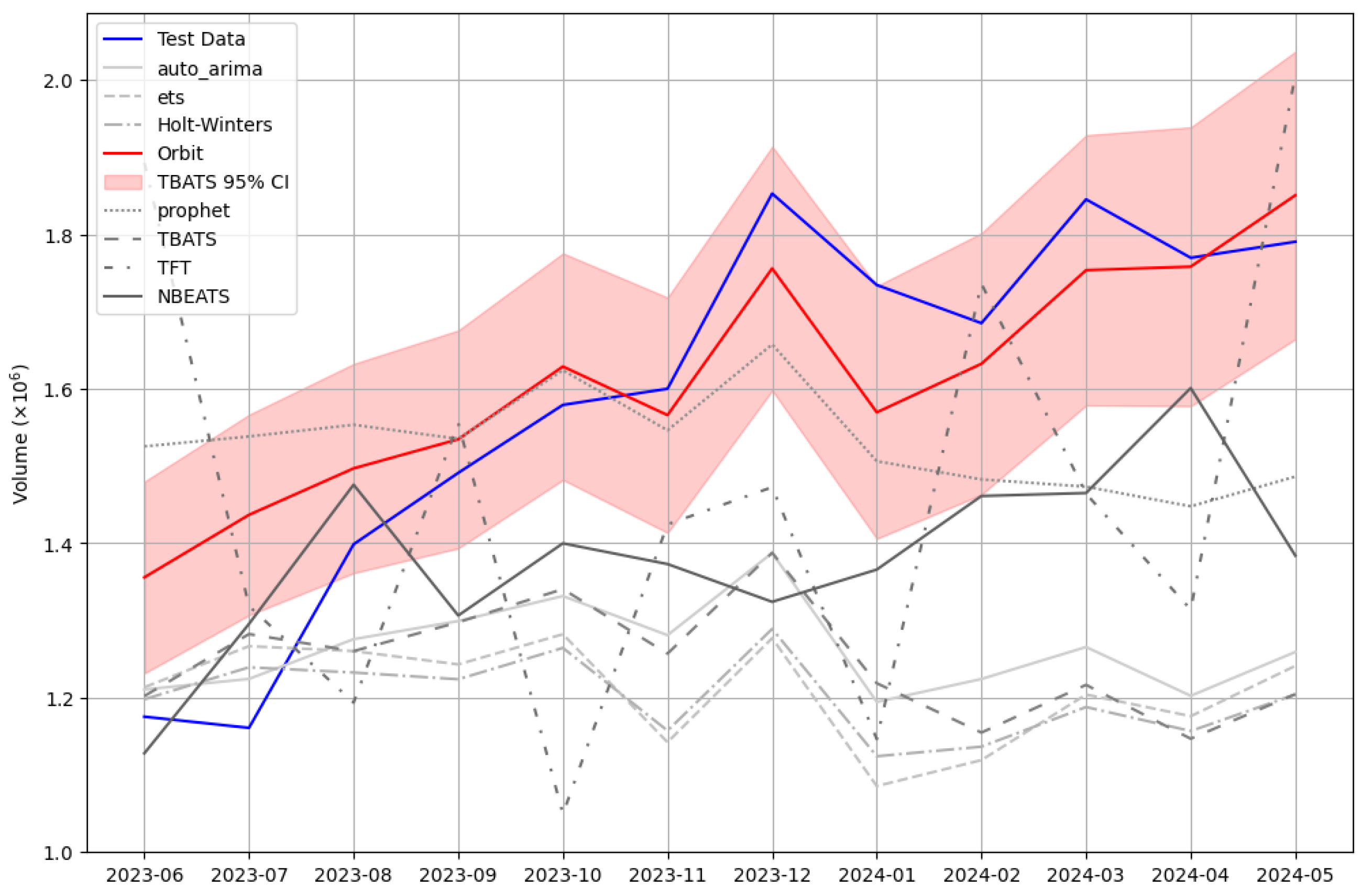
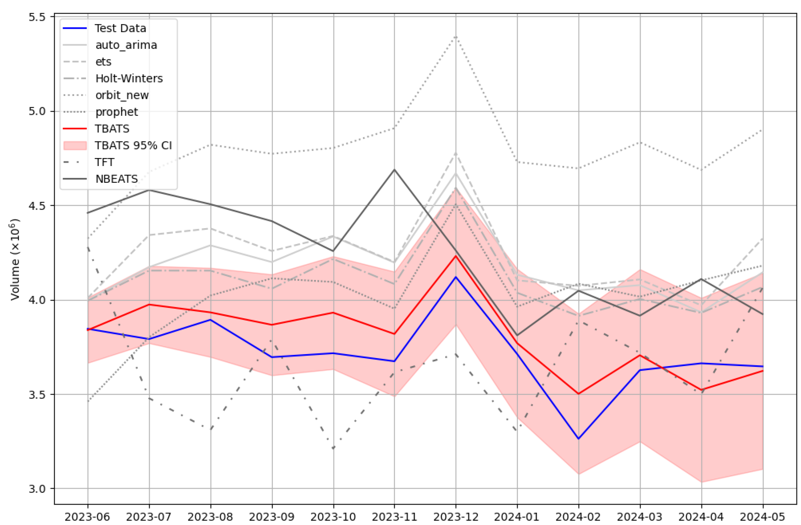
The best models identified for each series were Orbit (263) for ethanol, with a percentage error of 6.77% (Figure 5), and TBATS (144) for gasoline, with a percentage error of 3.22% (Figure 6). Both models presented significant values when evaluating the residuals using the Ljung–Box test, indicating that the residuals exhibit a white noise pattern. This suggests that the model parameters are well-fitted to the data; therefore, these models can be reliably used for accurate forecasting.

The test data in the gasoline and ethanol cases are in blue, while the best-performing model’s forecast data are shown in red. Additionally, a 95% confidence interval for the best model’s forecast is highlighted in the plot using a red-shaded region. This confidence interval visually represents the uncertainty around the model’s predictions, showing the range within which the true values are expected to lie with 95% probability.

In agreement with the results for ethanol found in Table 5, the Orbit model is the one that best fits the validation sample in Figure 5, which displays the forecast of each model in the best window for the ethanol time–series. The Orbit and TFT models presented the most optimistic forecast results when comparing the forecast models with the last 12 months of validation. In contrast, the ARIMA, ETS, Prophet, Holt–Winters, TBATS, and NBEATS models generally demonstrated more pessimistic forecasts than the test sample values.

The graph showing the gasoline validation sample was plotted with the results of the forecasting models in Figure 6. The ARIMA, ETS, Holt–Winters, TBATS, Orbit, and NBEATS models provided more optimistic forecasts than the validation data, while the TFT model was slightly more pessimistic.

The choice of training window and the characteristics of the time–series impact the type of forecasting model to be used. It is important to compare models and tailor them to each specific scenario for more accurate and reliable results. Considering a 144-month time frame for ethanol, the NBEATS model was the best performer. However, based on the overall results, it can be inferred that none of the machine learning models (TFT and NBEATS) excelled in analyzing the Brazilian gasoline and ethanol sales volume despite achieving good results. The econometric adjustment models yielded better results in time–series analysis.

5.2. Forecasting with the Selected Model

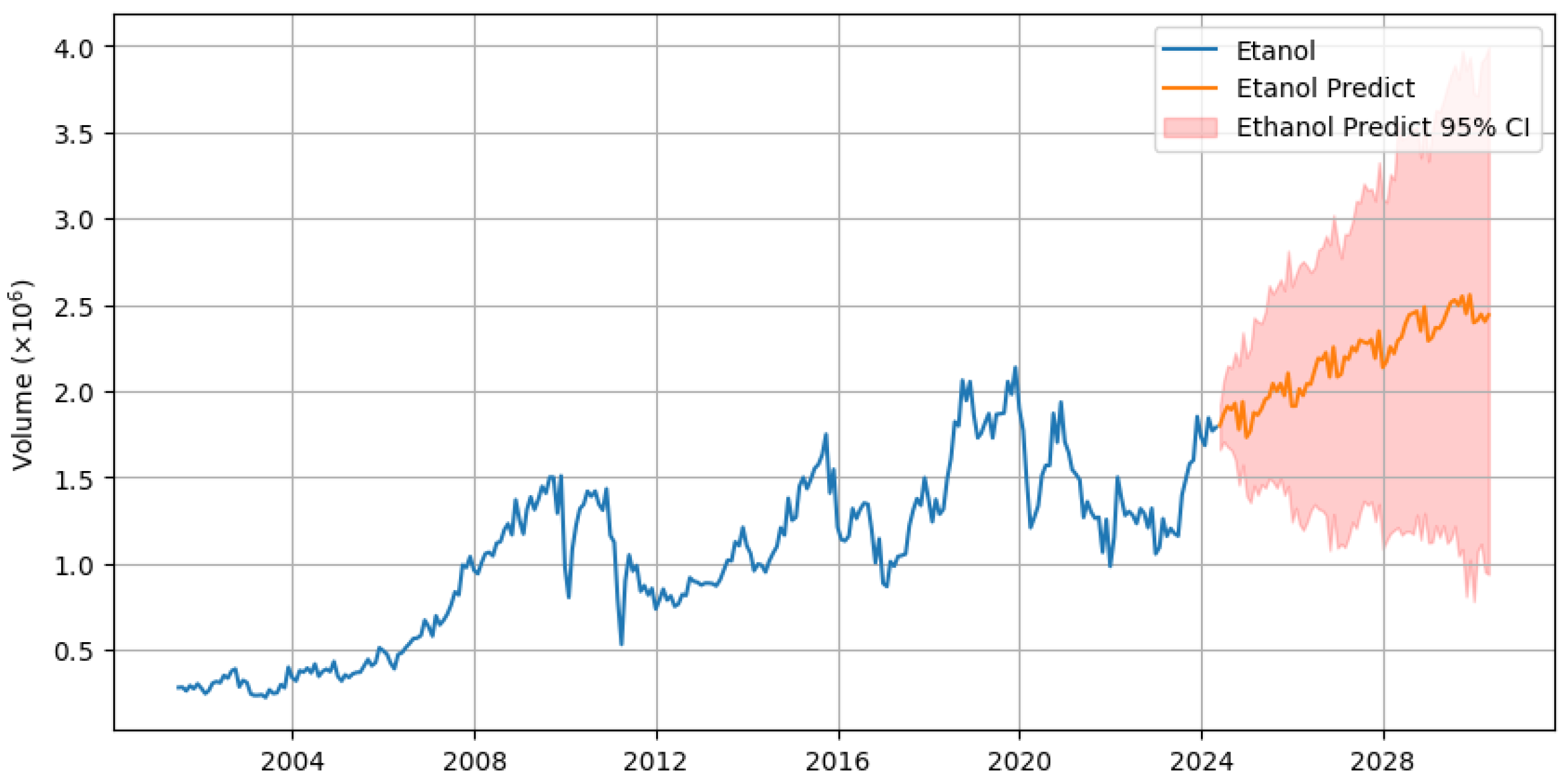
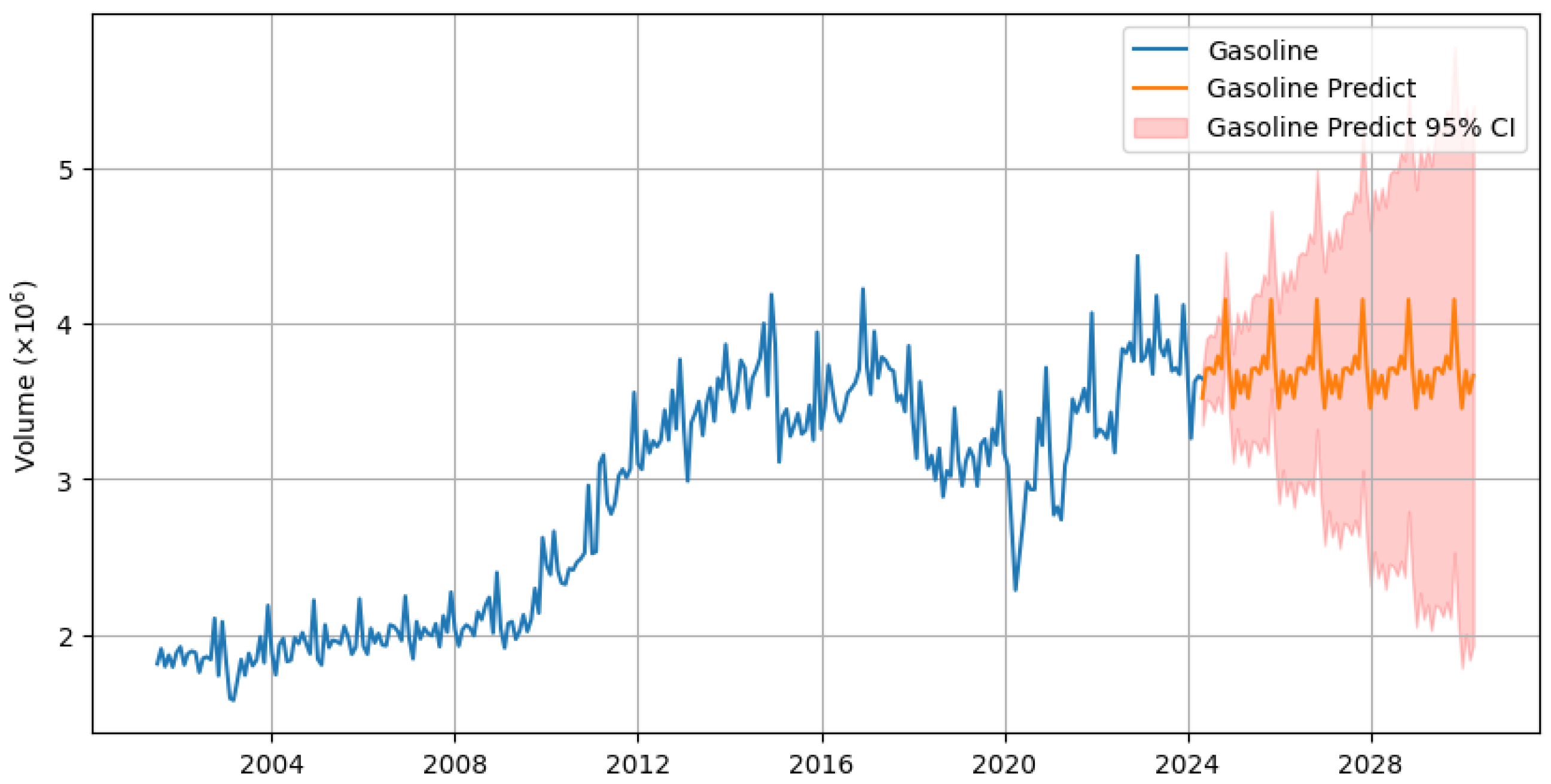
This subsection presents the application of the selected best forecasting model for the ethanol and gasoline variables from 2024 to 2030. This section refers to Step 4 of Figure 1. It presents the use of the Orbit model (263) for the forecast of ethanol and the TBATS model (144) for the estimates of gasoline, based on the performance results found in Section 5.1.

Based on the selected forecasting models, the prediction results are displayed in Figure 7 for ethanol and Figure 8 for gasoline. These figures visually represent the expected future trends for both fuel types. The forecast for ethanol suggests a significant increase in consumption, with a projected peak exceeding 2 million liters per month. This indicates a potential rise in demand for ethanol production, which could be attributed to factors such as shifts in consumer preferences towards biofuels, government incentives for renewable energy, or seasonal production cycles in the agricultural sector that support ethanol production.

The forecast also shows a notable upward trend for gasoline, with consumption predicted to surpass 4 million liters monthly. This trend may be driven by population growth, increased vehicle usage, or fluctuations in global oil prices that affect gasoline consumption patterns. Understanding these forecasts is essential for stakeholders, including fuel producers, policymakers, and economists, as they provide information on the potential future supply–demand dynamics in the fuel market.

Additionally, the forecasts evidence the importance of monitoring external variables, such as changes in transportation habits, technological advancements in alternative energy sources, and economic conditions, which could further influence the trajectory of fuel consumption. Analyzing the peaks and patterns highlighted in the figures allows for informed decisions regarding production planning, inventory management, and energy policy.

In conclusion, the forecast peaks in ethanol and gasoline consumption emphasize the growing demand for energy resources and highlight the need for strategic planning to balance supply and demand. These results can also serve as a foundation for future research on optimizing fuel distribution and exploring sustainable energy alternatives.

Ethanol and gasoline exhibit different behavioral patterns when analyzed based on the applied forecasts for each time–series. The new estimates of the current study for the period up to 2030 are more pessimistic than the scenario presented about two decades ago by previous studies [26]. With a forecast for 2006 to 2012, there was an expectation of growth in ethanol consumption if Brazil maintained an optimistic GDP growth rate. However, the 2008 crisis certainly caused instability in the ethanol sales market. Despite the recovery of GDP within the forecast period, there was no significant increase in ethanol until 2012, but rather an increase in gasoline sales consumption.

The results found that ethanol consumption should decrease until 2026, followed by a recovery period. After that, it should decline until 2028, with two more recovery periods until 2030. Sales volume is not expected to exceed ethanol, and an increased volume trend among consumers was identified during the study period. The gasoline sales volume is significantly lower without ethanol and will grow considerably until 2030. Although sales should peak yearly for seasonal reasons, they are not projected to exceed previously observed sales levels. There is no evidence to indicate a reduction in the consumption of fossil fuels, despite the recent electrification of vehicles.

5.3. Discussion of the Results

Brazil is one of the world’s leading producers and consumers of ethanol, and ethanol is often viewed as a substitute for gasoline. Furthermore, gasoline sold in gas stations throughout the country contains an ethanol blend of 27%. However, there are differences in the behavior patterns of each time–series, as well as in the performance of each model, the performance within each training window sample, and the behavior patterns of the applied forecasts.

The Brazilian energy scenario is uncertain. The results indicate that the country will likely continue to rely on fossil fuels in the upcoming years. Promoting alternative methods to change consumer behavior effectively can be challenging. Fuel consumption is inherently linked to Brazil’s entire supply chain, which relies heavily on a fleet of trucks to transport food, goods, industrial products, and raw materials. Therefore, it is relevant to introduce measures that encourage the use of ethanol or other environmentally friendly alternative fuels.

Since current pricing policies have not effectively influenced consumer behavior, this objective can be achieved by implementing pricing strategies that align with international market prices. In addition, promoting changes in consumer culture by encouraging the cultivation of sugarcane plantations for ethanol production through investments in local economies could increase ethanol consumption, as these agricultural regions would also benefit from consumption [41].

Another option would be to reduce gasoline consumption by promoting hybrid cars, hydrogen engines, and other more efficient vehicles. In addition to the already known solution of improving the structure of public transport—which has already been gradually adapted to the use of alcohol, making it a more attractive solution for more people—this would reduce the number of cars in circulation daily and improve the fluidity of traffic in the central Brazilian capitals. This would also reduce the consumption of fossil fuels.

In addition to promoting research to develop new technologies to increase the efficiency of ethanol engines, although the ethanol currently available on the market is already of high quality, incorporating new research improves understanding of changes in Brazilian consumer behavior by promoting a better perception of the social, environmental, and economic benefits of using cleaner fuels.

6. Conclusions and Future Works

The debate on alternative energy sources is related to the issues associated with sustainable development, and the expansion of energy is relevant in significantly influencing the complex dynamics of the market. Fluctuations concerning the price of oil can have an impact on a myriad of activities, particularly in the context of Brazil and its unique economic landscape. Biofuels, with a particular emphasis on ethanol, have been empirically demonstrated to serve as a viable alternative to traditional fossil fuels; from this analytical perspective, it can be posited that the level of energy security is experiencing a notable increase.

From the perspective of fuel demand in Brazil, especially gasoline and ethanol, recent studies seek to explain the relationship between these goods to find the degree of substitution between them. This approach gains emphasis when analyzed together with sustainability issues, a subject that has permeated the center of several discussions. As a non-renewable fuel, gasoline is likely to become scarce in the future, although this perspective cannot be described as a consensus in the literature.

Ethanol and gasoline are the primary energy sources within the contemporary energy paradigm. They are essential transportation components and underpin various economic and industrial processes. As a biofuel, ethanol exhibits a diminished carbon footprint relative to gasoline, facilitating the reduction in greenhouse gas emissions and advancing the transition toward cleaner energy alternatives.

Advocating for ethanol instead of gasoline aligns with the objectives posited by Sustainable Development Goal 7 (SDG 7). Ethanol is a renewable resource that mitigates reliance on fossil fuels and presents a cleaner and more sustainable alternative. This objective aspires to achieve universal accessibility to affordable, reliable, and sustainable energy by 2030.

However, consumer behavior when choosing between the two goods is one of the central problems in this context, which can determine the intensity of the effects of policies specifically targeted at the sector. Thus, ethanol can only compete with gasoline in or near production centers. In other words, demand is repressed in some states despite the various benefits compared to gasoline consumption. The authors also note that, in some cases, ethanol is only competitive seasonally during harvest periods.

This study identified Uber Orbit as the most accurate model for ethanol forecasting, achieving a MAPE of 6.77%, and TBATS as the top-performing model for gasoline, with a MAPE of 3.22%. Based on these models, ethanol sales are projected to exceed 1.75 million liters by 2030, while gasoline consumption is expected to peak above 4 million liters, influenced by seasonal variations. These forecasts indicate that most fuel consumption will continue to be dominated by non-green fuels, such as gasoline, rather than ethanol, underscoring the ongoing challenge of transitioning to more sustainable energy sources.

In future work, the authors suggest considering exogenous variables in the prediction to regularly update models, conduct scenario analyses, and monitor consumer behavior to improve the adaptability of forecasts. The variables may be selected using a Granger causality test. Such an analysis could reveal the different reactions to the consumption of these fuels in response to the variation of economic, industrial, and climatic variables, thus enabling simulations on the variation of demand for ethanol and gasoline in response to these exogenous variables. Extensions to this research can be made by including new explanatory variables in the demand system, such as the prices and quantities demanded for other fuels, vehicle fleets, and variables related to the external sector. The latter is intended to control exogenous effects on demand.