A Reduced-Order Algorithm for a Digital Twin Model of Ultra-High-Voltage Valve-Side Bushing Considering Spatio-Temporal Non-Uniformity

Abstract

The valve-side bushing of a converter transformer is a critical component in ultra-high-voltage direct current (UHVDC) systems, making its monitoring through digital twin technology highly significant. However, the complex structure and spatio-temporal nonlinearity of the bushing result in a large computational demand for its digital twin model, which requires an effective order reduction algorithm. This paper proposes a Spatio-temporal Non-uniformity Proper Orthogonal Decomposition (SN-POD) algorithm considering the inhomogeneity of space and time consumption to meet the reduced-order computational requirements of UHV valve-side bushings. This proposed method reduces the calculation time to 10% of the full-order simulation model while controlling the error range of the key research area less than 0.1%. The test results show that this method has good robustness, calculation speed, and accuracy. This research can significantly enhance the computational efficiency of digital twin modeling for valve-side bushings and provide a technical foundation for constructing digital twin models for UHV valve-side bushings.

1. Introduction

Ultra-high-voltage direct current (UHVDC) transmission plays a key role in optimizing large-scale cross-regional resource allocation [1]. As the key weak link [2], the valve-side bushing of a converter transformer urgently requires an optimized design to enhance the operation and development of HVDC technology [3]. Due to the simplicity, economy, and high efficiency of digital twin technology [4], it can improve the design efficiency of valve-side bushings and ensure the safety level of the UHVDC system in industrial applications [5]. The complex structure, mechanism, and internal operating environment of UHV valve-side bushings leads to an enormous computational demand for digital twin models [6]. Hence, it is necessary to develop an efficient reduced-order algorithm capable of fast physical field calculations, which reduces the full-order model (FOM) to a reduced-order model (ROM). The ROM serves as a critical physics-driven component of digital twin models, enabling their practical implementation. By integrating the ROM with real-time data interfaces, dynamic updates to digital twin models can be achieved, ensuring both computational efficiency and adaptability in operational scenarios.

The reduced-order algorithm used in physical field calculations, which reflects the real-time response level of the twin model to disturbance signals, is one of the key indicators of the quality of digital twin models for valve-side bushings. All in all, these fast calculation methods could be divided into two categories: data-based and physics-based.

Data-driven methods only need to realize the dynamic behavior decomposition and predict the future state based on the data characteristics in the calculation. Sharak [7] and Yang [8] proposed to use Dynamic Mode Decomposition (DMD) to predict future states with the time-series snapshot data. While unsupervised methods can extract intrinsic system modes from dynamic snapshots without labeled data, their predictive capabilities are constrained by linear approximation assumptions and data completeness requirements. For strongly nonlinear coupled or high-dimensional parametrized problems, supervised learning enhances the reduced-order modeling accuracy by integrating physical constraints and data labels. Zhao [9] constructed a multi-wind-speed nonlinear unsteady aerodynamic ROM based on the LSTM deep neural network. Brivio [10] proposed a pre-trained physics-informed deep learning ROM (PTPI-DL-ROMs) for solving nonlinear parameterized partial differential equations, which effectively integrates physical principles with data-driven approaches, alleviates computational burdens, and exhibits high accuracy and efficiency across multiple test cases. Xie [11] proposed a deep residual neural network (ResNet) closure learning framework for reduced-order models of nonlinear systems. Fresca [12] proposed a deep learning-based reduced-order model (DL-ROM) to address the limitations of conventional reduced-order modeling techniques when dealing with nonlinear time-dependent parametrized PDEs. Although the data-driven methods circumvent the stiffness matrix reconstruction process, they entail substantial data dependencies, requiring extensive training datasets to develop black-box predictors, with sample size demands typically larger than those of physics-based methods.

Physics-based methods are often applied to scenarios that have certain requirements for physical calculations. In conventional finite element analysis frameworks, adaptive time-stepping strategies can optimize computational efficiency and reduce redundant iterations through a dynamic adjustment of step sizes [13,14,15]. While this approach effectively decreases convergence iterations, the computational complexity remains of the same order as the original system, particularly imposing substantial hardware burdens for large-scale engineering simulations. To fundamentally reduce the computational complexity, model order reduction methodologies based on modal space mapping have been developed. Proper Orthogonal Decomposition (POD) is one of the most used physics-driven methods for implementing model order reduction [16], widely applied in fields such as dynamics [17] and aerospace [18]. Li [19] developed a ROM for Maxwell’s equations by integrating POD with an adaptive snapshot selection strategy. References [20,21,22] proposed to use POD in the calculation of transformers’ temperature field. Wang [23] applied POD to the finite element rapid computation in ±400 kV converter transformer valve-side bushings. Yang [24] proposed a snapshot partition POD (SP-POD) to achieve the calculation of a valve-side bushing based on the quantity gradient of each node in the snapshot. The comparation of typical fast calculation methods are shown in

Table 1. Comparative analysis of typical fast calculation methods.

	Method	Algorithm Complexity	Training Data	Speed	Accuracy
Data-driven methods	DL [9,10,11,12]	Very high	Very Large	Very Fast	Very High
	DMD [7,8]	Medium	Large	Very Fast	High
Physics-based methods	Adaptive steps [13,14,15]	Low	-	Slow	High
	POD [19,20,21,22,23]	Medium	Very Low	Fast	High
	SP-POD [24]	High	Very Low	Fast	High

. So far, there are still few studies on the reduction calculation of valve-side bushings. The POD method achieves an optimal balance among computational speed (fast), accuracy (high), and data requirements (very low), making it particularly suitable for power equipment scenarios that require both physical interpretability and real-time performance.

The characteristics of those physics-based methods are listed as follows:

(1)

Most methods use POD directly but can be further optimized for valve-side bushings, given their elongated structure and highly refined components.

(2)

Those methods mainly focus on an improvement at the algorithm level without considering the influence of the physical mechanism, particularly neglecting the uneven distribution in time and space.

(3)

Only a few methods are applied to the valve-side bushing.

In summary, the research on ROM for UHV valve-side bushings remains limited and is still in the early stages, necessitating further in-depth exploration.

In this paper, a reduced-order digital twin algorithm accounting for spatial and temporal non-uniformities is studied and proposed in Section 2. The proposed algorithm is validated and analyzed in Section 3. Section 4 discusses the sensitivity of the proposed method. Section 5 concludes this paper.

2. The Reduction Algorithm Method Considering Spatio-Temporal Non-Uniformity

2.1. The SVD Decomposition Method for Spatio-Temporal Non-Uniformity

For power equipment data, where the spatial dimension greatly exceeds the number of temporal sampling points, the conventional POD method incurs significant computational costs, resulting in reduced efficiency. Therefore, it is necessary to improve the classical POD method. Yan [25] proposed a Singular Value Decomposition (SVD)-based POD method, which simplifies certain steps in the conventional POD method. Moreover, the eigenvalues generated by the SVD method are derived from the squares of the singular values, eliminating negative values and automatically arranging the values in descending order. For these reasons, the SVD-POD method is ultimately selected to achieve a ROM for the digital twin model of the UHV valve-side bushing.

At a certain moment, physical quantities, such as temperature or electric potential values, are collected from m different positions on the valve-side bushing. If the data are collected at n different time instants, an n × m times instantaneous matrix, U(t,x), can be constructed. This matrix can be further expressed as the sum of the mean matrix of the physical quantities, Ū(t,x), and the fluctuation matrix of the physical quantities, U⁰(t,x), as (1).

$$U(t,x)=\overline{U}(t,x)+U^0(t,x)$$

(1)

The key to model reduction lies in retaining the most significant parts of the U⁰(t,x) matrix that contribute effectively to the overall behavior while eliminating less influential components. Based on the SVD decomposition, three distinct matrices are obtained as (2), where B is a n × n times matrix representing the times mode structure, V is a m × m square matrix of temporal modes, and S is a n × m spatial diagonal matrix containing an eigenvalue.

$$U^0(t,x)=\mathit{B}\mathit{S}{\mathit{V}}^T$$

(2)

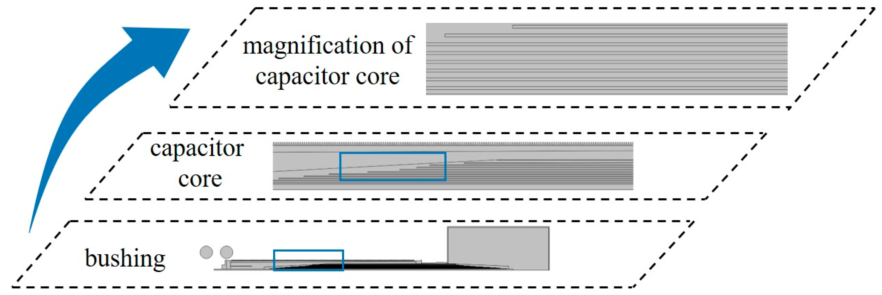
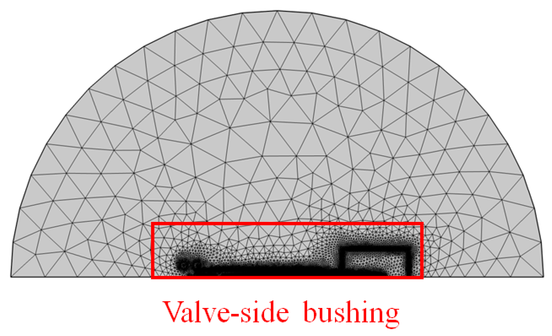
The SVD-POD method treats the reduced-order object, assuming spatial and temporal uniformity. However, due to the unique structure and operational characteristics of the valve-side bushing, this assumption is not entirely applicable. Spatially, as shown in Figure 1, certain structural components, such as the capacitor core, require more attention compared to other parts. For instance, extensive operational experience indicates that the capacitor core, as the primary component of the valve-side bushing, is prone to dielectric loss under the influence of higher harmonics, leading to the overheating and insulation failure of the capacitor core.

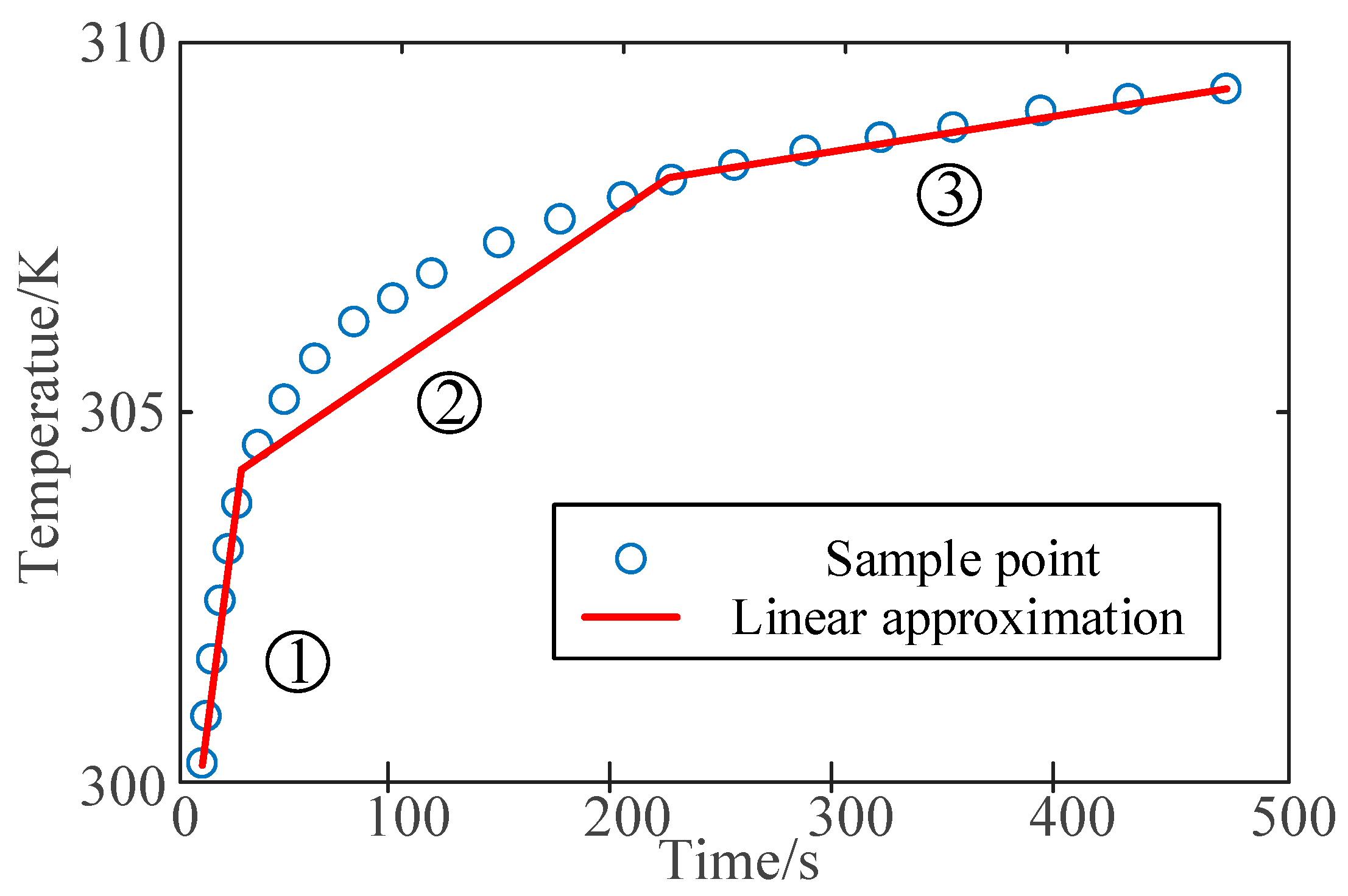
Temporally, under special operating conditions, such as sudden excitation, short circuits, or polarity reversals, higher sampling frequencies are required to capture changes in the physical quantities inside and outside the bushing [26]. This means that points with strong nonlinear variations need more sampling points, while points with weaker nonlinear variations can have fewer sampling points. Take the temperature variation of the bushing as an example, shown in Figure 2. Segments ① and ③ can be approximated with linear functions, whereas segment ② would result in significant errors if represented by a linear function.

2.2. Sub-Regional Spatial Decomposition

In (1), the physical quantities of the valve-side bushing in the POD are represented as the sum of the mean matrix of the physical quantities, Ū(t,x), and the fluctuation matrix, U⁰(t,x). However, during the computational process, only U⁰(t,x) is subjected to modal decomposition. Therefore, the physical quantities contained in the original fluctuation matrix can be processed in sub-regions.

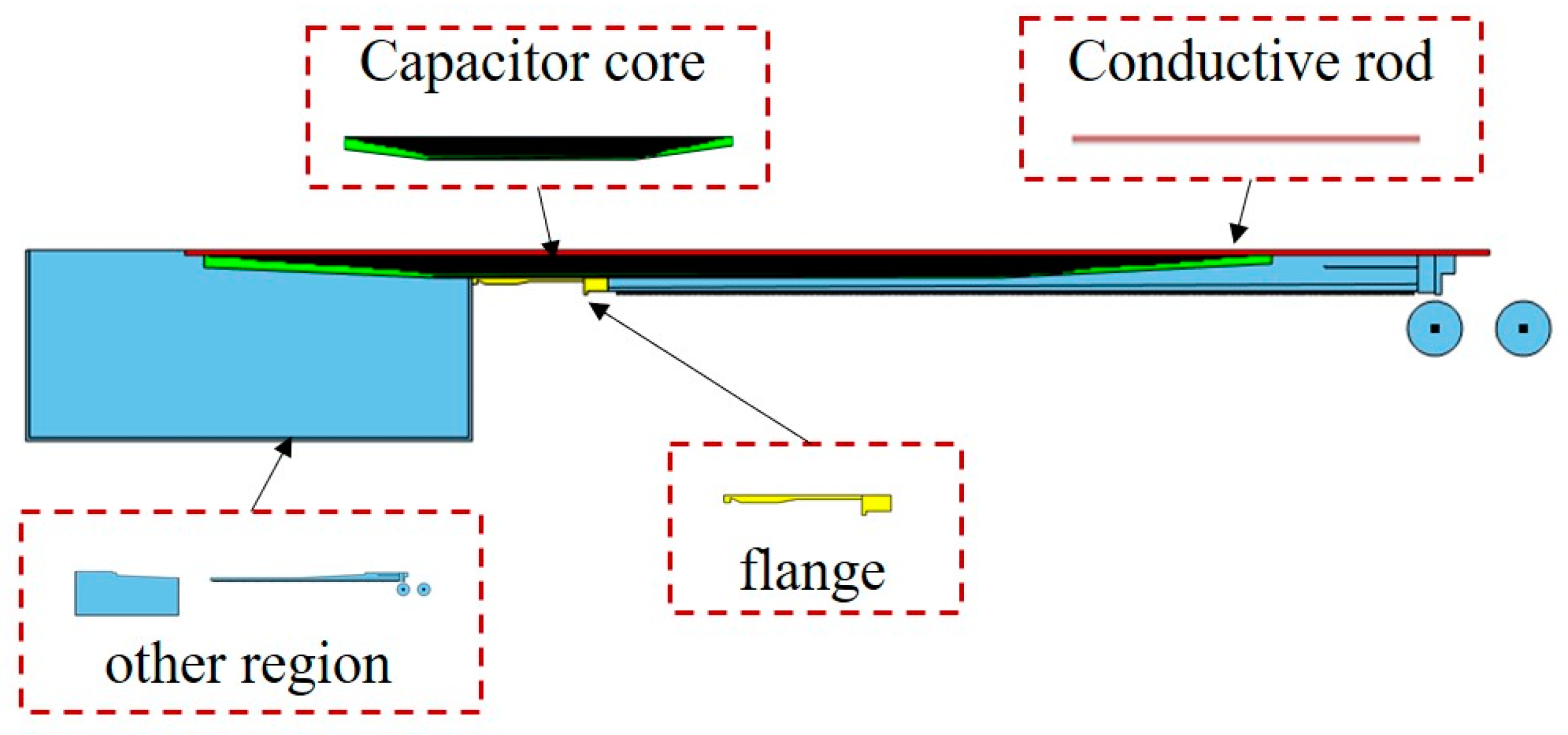
In this study, using the electrothermal field as an example, an appropriate algorithm is developed. The regional distribution settings for the bushing can be divided into four sub-regions based on the field gradient, as shown in Figure 3. The conductive rod exhibits a pronounced temperature gradient due to its upper section being exposed to ambient air and the lower section immersed in high-temperature transformer oil, compounded by internal high-intensity heat generation. As an equipotential body, it maintains a relatively low electric field gradient [27]. The flange, functioning as a grounded equipotential component, demonstrates a significant temperature gradient despite its connection to the high-temperature oil tank and exposure to ambient air, yet its electric field gradient remains minimal due to the absence of potential differences. The capacitor core represents the most complex field distribution region, where direct contact with the high-potential conductor internally and grounding through the end screen externally creates dual effects of significant temperature gradients and electric field gradients [28]. Other regions exhibit moderate gradient intensities in both thermal and electric fields, primarily influenced by coupled field interactions with adjacent components.

For regional partitioning, two methods are proposed. Take the four sub-regions divided in the bushing example above.

The instantaneous fluctuation matrix for different regions is represented as (3).

$$U_i(t,x)=\left[\begin{array}{ccc}{U}_i(t_1,x_1)& \cdots & U_i(t_1,x_{m_i})\\ ⋮& \ddots & ⋮\\ U_i(t_n,x_1)& \cdots & U_i(t_n,x_{m_i})\end{array}\right]$$

(3)

U_i(t,x) represents the instantaneous fluctuation matrix for the i-th region. For example, the valve-side bushing is divided into four areas while U₁(t,x) corresponds to the data from the central conductor region. Consequently, the entire instantaneous fluctuation matrix, U⁰(t,x), can be represented in a block form as (4):

$$U^0(t,x)=\left[\begin{array}{cccc}{U}_1(t,x)& U_2(t,x)& U_3(t,x)& U_4(t,x)\end{array}\right]$$

(4)

Since the matrices requiring a modal decomposition are the sub-matrices, Ui, their spatial dimensions are m_i, with m_i reflecting the importance of the corresponding region. According to (4), the total spatial dimension of U⁰(t,x) is m = m₁ + m₂ + m₃ + m₄, where m_i < m. By employing a sub-regional division strategy, this method decomposes the total dimension, m, into smaller sub-dimensions, m_i, significantly reducing the spatial dimensionality of the matrices for modal decomposition compared to the conventional approach (zeroing out non-sub-regions while retaining the original dimension, m_i << m), which drastically lowers the computational complexity. This sub-regional sampling approach preserves critical regional information while avoiding the high computational cost of full-dimensional matrix operations, thereby enhancing the overall analysis efficiency.

2.3. Discrete Time Sampling

To address the coupled effects of multi-physical fields inside the bushing, such as the nonlinear coupling between non-uniform electric and temperature fields, it is necessary to increase the sampling frequency for points where the physical quantities exhibit strong nonlinear temporal variations. The Latin Hypercube Sampling (LHS) method [29] based on Monte Carlo principles, incorporating the idea of stratified sampling, has been used in this paper. LHS utilizes a stratified sampling mechanism to enhance coverage uniformity across individual parameter domains. However, this methodology cannot ensure optimal space-filling properties in multivariate contexts. Its sampling efficacy exhibits progressive degradation with dimensional expansion [30]. Notably, in the time dimension sampling of this study, as a univariate application scenario, LHS effectively prevents sample omissions in tail regions [31].

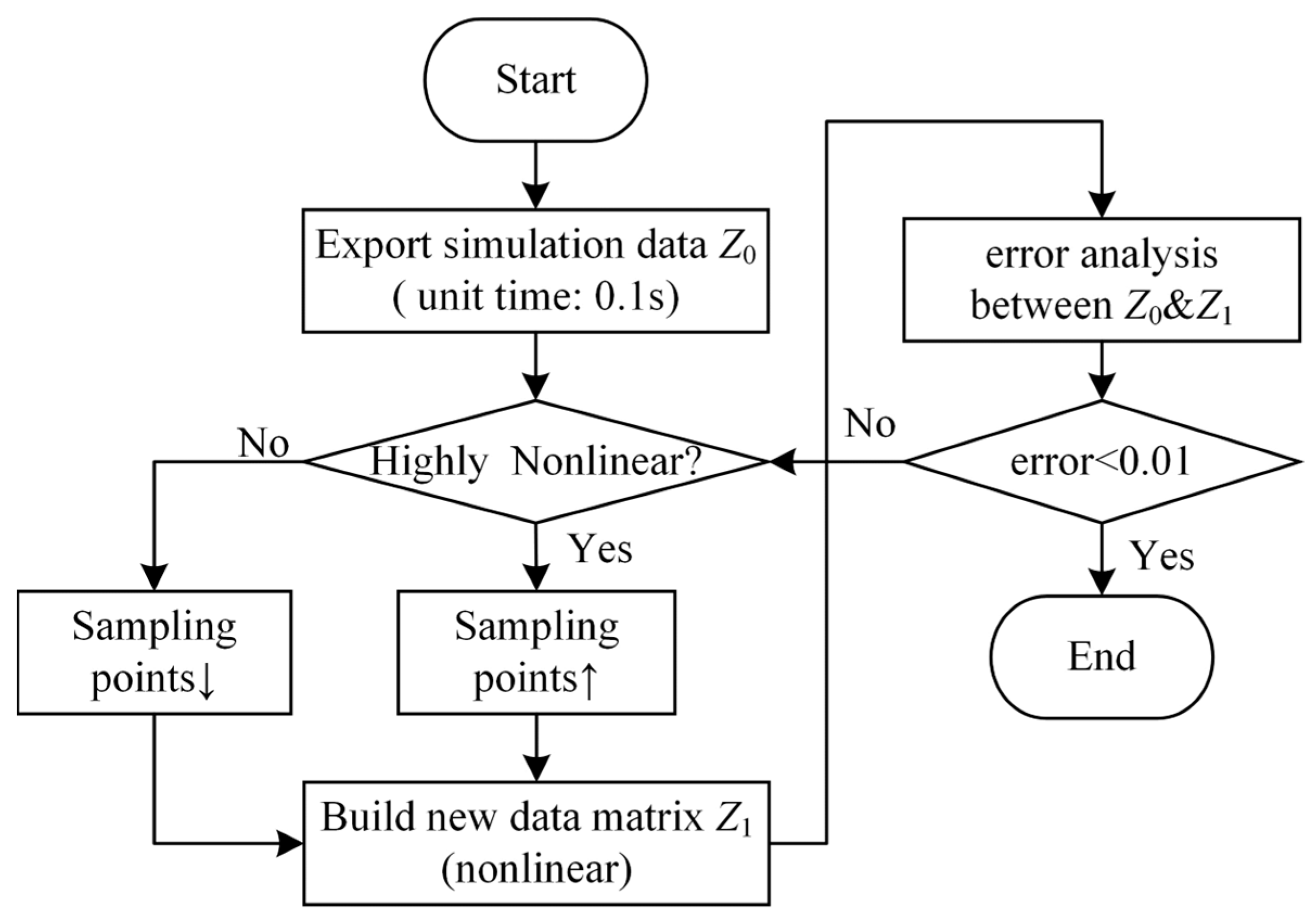
The first step is to preprocess the computational data, Z₀, of the valve-side bushing digital twin model to identify and separate regions with strong nonlinear variations from those with weak nonlinear variations. Subsequently, the two regions are resampled in the time dimension. Typically, there is no fixed standard to determine whether the number of sampling points is sufficient. Therefore, after exporting the full-order data, Z₁, of the valve-side bushing, sampling points are incrementally added based on experience, starting from a small number and gradually increasing. The sampled data are then fitted, and the error compared to the full-order data is evaluated. If the error falls within an acceptable range, the sampling points are deemed sufficient. Ultimately, this iterative sampling process reduces the data volume. The specific workflow is shown in Figure 4.

Consider a probability problem with a total of M random variables, X₁, X₂,…, X_M. Let X_m be one of these random variables, and its cumulative distribution function [32] is given by:

$${{\displaystyle Y}}_m={{\displaystyle F}}_m({{\displaystyle X}}_m)$$

(5)

Let the number of samples be N by dividing the vertical axis of the cumulative distribution function Y_m into N equal intervals, each with a width of 1/N, and sampling once within each interval.

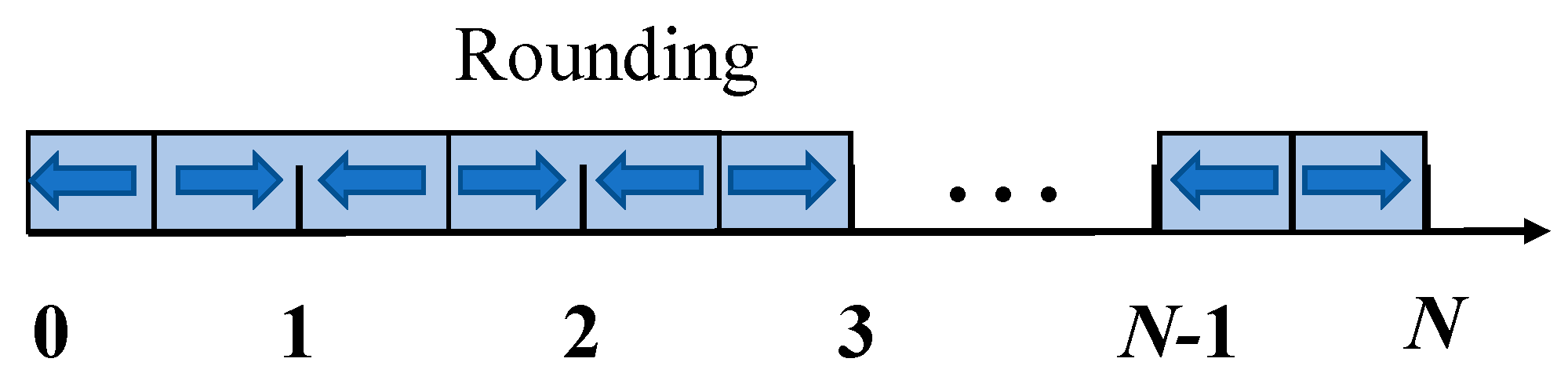
The sampling points in this study are jointly determined by the spatial distribution of valve-side bushings and temporal sequences in numerical simulations. For spatial dimension discretization, a sub-region processing method employing multi-scale grid partitioning is implemented. Regarding the temporal dimension, this paper proposes a hybrid approach based on one-dimensional LHS: First, the nonlinear physical quantities of valve-side bushings are modeled as cumulative probability distribution functions with time as the input parameter. Subsequently, the total time interval is divided into N equidistant sub-intervals, within which random sampling is conducted using LHS. To accommodate the discrete time-step characteristics inherent in numerical simulation systems, a nearest-integer rounding operation is applied to map the continuous temporal sampling values to integer time nodes. The complete implementation workflow is illustrated in Figure 5.

The original input data are sequentially arranged in chronological order. However, the data sampled via LHS are no longer sorted by the original time sequence. Hence, the sampled data need to be reordered by evaluating the magnitude of the time values, ensuring that the predicted physical quantity variations align with the actual variation patterns. By increasing the sampling points for time periods with strong nonlinear variations under special operating conditions, the loss of information on physical quantity variations is minimized. As a result, the final accuracy of the predictions is significantly improved.

2.4. Spatio-Temporal Non-Uniform POD Model and Computational Workflow

In general, the computation process of the ROM can be divided into two stages: the offline stage and the online stage. The offline stage involves the use of the FOM to comprehensively reflect the physical laws related to the valve-side bushing through finite elements and other algorithms. Although this stage involves a high computational workload and long computation time, often lasting several hours or even days, it achieves high computational accuracy. The precise offline computation results provide sample data for the online stage. The online stage, on the other hand, is based on the ROM. By solving the approximate model after a reduction, it enables a fast computational analysis of the digital twin model [33].

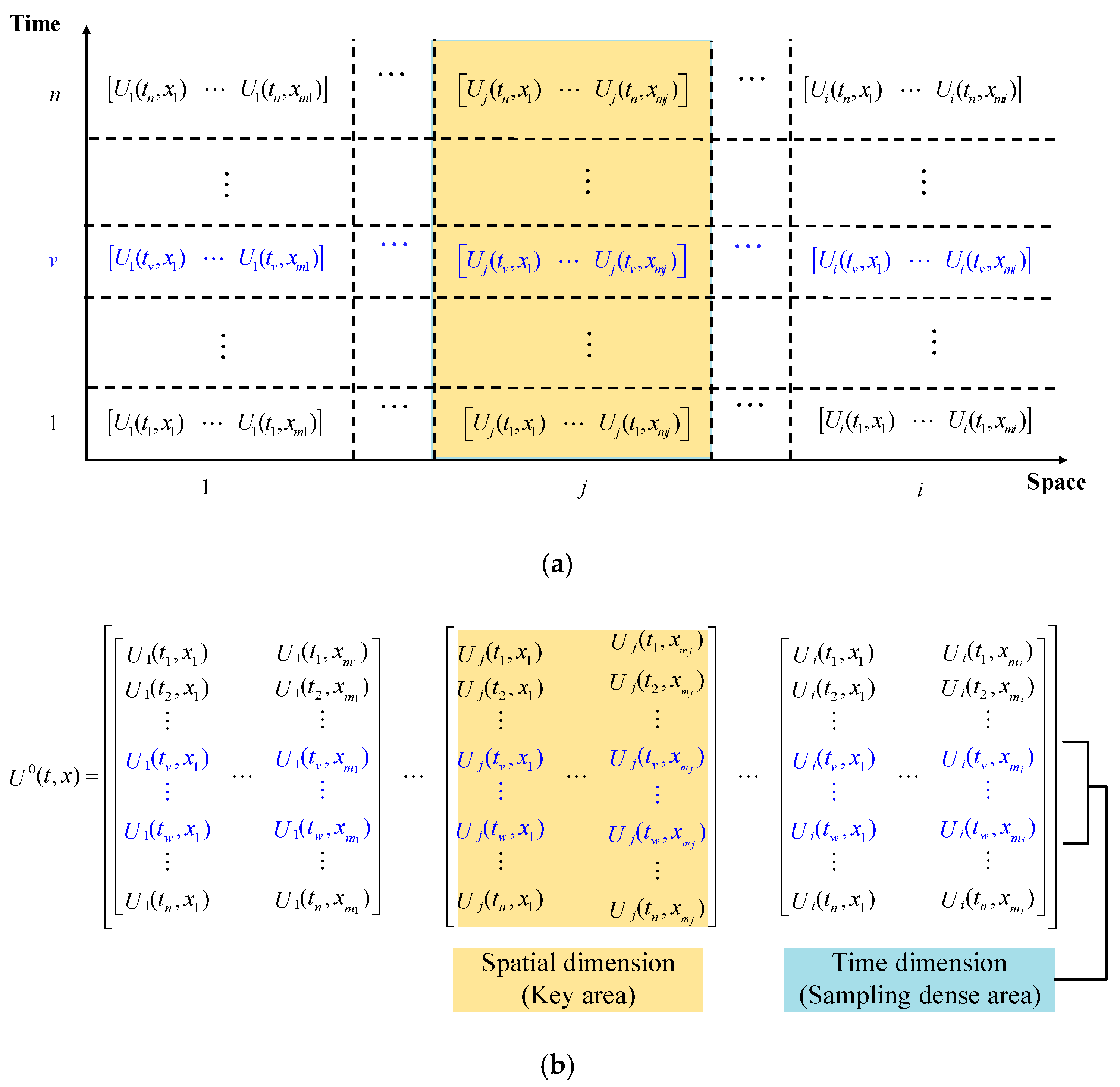
The spatio-temporal non-uniform POD (SN-POD) constructs a decomposable matrix in the ith sub-region by considering the actual variations in both the temporal and spatial dimensions. Temporally, intensive sampling is performed during time intervals with strong nonlinear variations in physical quantities. For example, in segment ② of Figure 2, as (6), the time dimension forms a high-density sampling region represented by a blue area (from U_i(t_v,x₁) to U_i(t_x,x_mi)).

$$U_i(t,x)=\left[\begin{array}{ccc}{U}_i(t_1,x_1)& \cdots & U_i(t_1,x_{m_i})\\ ⋮& \ddots & ⋮\\ U_i(t_v,x_1)& \cdots & U_i(t_n,x_{m_i})\\ ⋮& \ddots & ⋮\\ U_i(t_w,x_1)& \cdots & U_i(t_w,x_{m_i})\\ ⋮& \ddots & ⋮\\ U_i(t_n,x_1)& \cdots & U_i(t_n,x_{m_i})\end{array}\right]$$

(6)

Within the spatio-temporal joint analysis framework, the matrix construction explicitly captures the non-uniform evolution characteristics of physical quantities across temporal and spatial dimensions. In the temporal dimension, the blue-highlighted segments indicate dense sampling regions, analogous to those depicted in Figure 6a. In the spatial dimension, matrix blocks of varying density are generated, reflecting differences in the criticality levels: high-importance regions (e.g., capacitor cores) exhibit a higher sampling density, while low-importance regions (e.g., flanges) employ sparser sampling.

Based on the analysis results in Section 2.2, the spatial dimension is further divided into sub-regions according to their importance. This results in a matrix that simultaneously accounts for spatio-temporal non-uniformity, as Figure 6b. This matrix represents the variation in physical quantities across the entire power equipment.

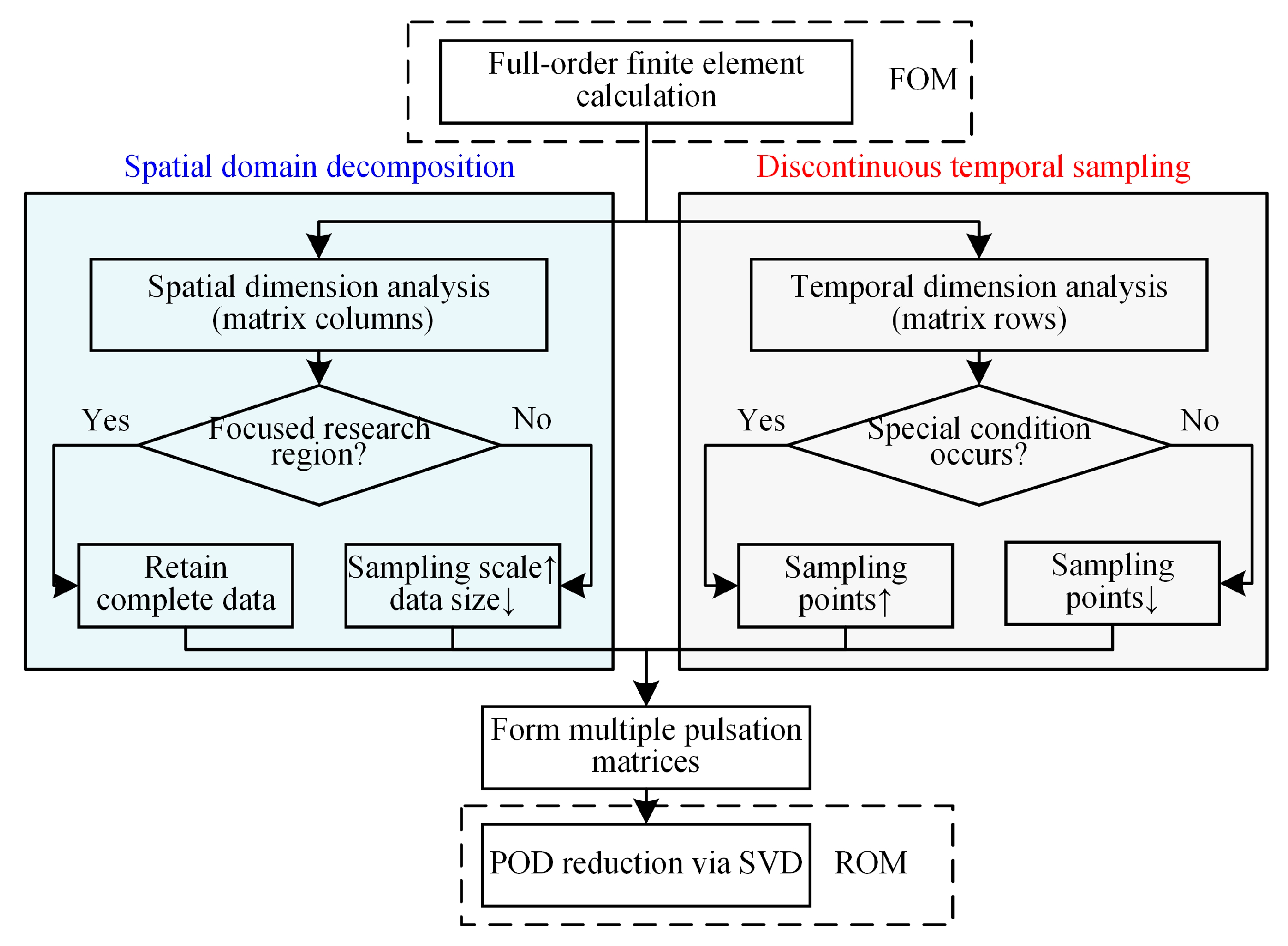
The workflow of SN-POD is shown in Figure 7.

3. Algorithm Validation

3.1. Model Construction

Based on the geometric drawings of the 1100 kV valve-side bushing provided by the bushing manufacturer, a geometric model of the 1100 kV valve-side bushing is constructed, as shown in Figure 8. For the potential conditions, the conductive rod of the bushing is set with a reversed polarity voltage for the entire rod, while the flange and end shield are grounded. The potentials of each layer of internal barriers in the bushing were coupled as floating conductors, with the innermost barrier was set to a high potential and the outermost barrier set to zero potential. The outer boundary of the air domain, defined as an infinitely distant reference point, has zero potential.

For the temperature field setup, the upper part of the valve-side bushing is inserted into the valve hall, where the external ambient temperature is set to 50 °C. The outer surface of the bushing in contact with the air is subjected to natural convection heat transfer, with a defined convection coefficient of 28 W/(m²·K). The lower part of the valve-side bushing is immersed in transformer oil, and the base of the bushing in contact with the transformer oil is set to a fixed temperature of 70 °C.

3.2. Results Analysis

The electric potential of valve-side bushings under normal operating conditions is analyzed based on the results of SN-POD. The selected comparison region is shown in Figure 9. The comparison of the computational results after applying the SN-POD reduction is illustrated in Figure 10. In Figure 10a, the electric potential cloud map at the top of the central conductor of the valve-side bushing is plotted using full-order data derived from finite element calculations in data processing software, representing the full-order electric potential cloud map. In Figure 10b, the cloud map of the electric potential is plotted using the same software based on the SN-POD results. A comparison between the two figs shows that the electric potential values are approximately the same, with the potential distribution and variation trends being consistent. The error in the highlighted region is 0.0178 kV (0.006%), which is within the acceptable range.

Figure 11a,b further provide a comparison of the electric potential and temperature at a specific sampling point of the valve-side bushing between the full-order simulation data and the results after applying SN-POD. The red solid line represents the full-order finite element results, while the blue dotted line represents the results of SN-POD. Clearly, the two curves in both figs almost completely overlap, demonstrating the feasibility and accuracy of the proposed method.

Figure 12 shows the temperature change in the valve-side bushing under excitation using SN-POD when the excitation is applied at·2.5 s. A comparison between Figure 12a,c reveals that the temperature range remains the same, and the temperature distribution and variation trends are consistent. The distribution of isothermal lines is also like the FOM. Figure 13 illustrates the variation in the electric potential and temperature, respectively, at a node near the surface of the high-voltage end of the valve-side bushing. The blue solid line represents the FOM results, while the blue data points represent the SN-POD results. Evidently, the two curves in both figs almost completely overlap. The maximum electric potential at the sampled point in the FOM is 1.14891 × 10⁶ V, while the maximum electric potential calculated by the SN-POD is 1.14902 × 10⁶ V, resulting in an error of only 0.1 kV (0.009%). Since no excitation is applied initially, the temperature remains stable at its initial value After the excitation is added, the temperature begins to rise and eventually stabilizes at approximately 301 K. As the focus is on regions with nonlinear variations, more sampling time points are allocated to the nonlinear regions.

Taking the 2D valve-side bushing model as an example, where normal excitation is applied at time 0 and additional excitation is applied at 2.5 s, the computational speed of the ROM compared to FOM is shown in Figure 14. Clearly, the SN-POD significantly improves the efficiency while meeting the accuracy requirements, and the computation time of the ROM is approximately 5% of the FOM.

The results show that the ROM reduces the calculation time of the FOM from the minute level to second level while maintaining accuracy, which effectively meets the dual requirements of accuracy and efficiency for the valve-side bushing digital twin model.

4. Discussion

4.1. The Impact of Different Workding Conditions

The instantaneous matrices formed by physical quantities are treated uniformly by SVD-POD, often resulting in lengthy overall computation times. In contrast, the SN-POD method allows for different processing approaches for different regions within the instantaneous matrix.

For example, for the capacitor core structure of the valve-side bushing, the error precision can be set as low as 0.01%. For other non-critical regions, the error range can be appropriately expanded. As a result, different regions of the valve-side bushing retain varying numbers of modes depending on their importance, as in Figure 15.

Based on the analysis above, after applying the SN-POD method, non-critical regions can adequately reflect their physical quantity variations, while critical regions meet the required precision and error thresholds. Hence, the computational efficiency of the SN-POD method could be significantly improved.

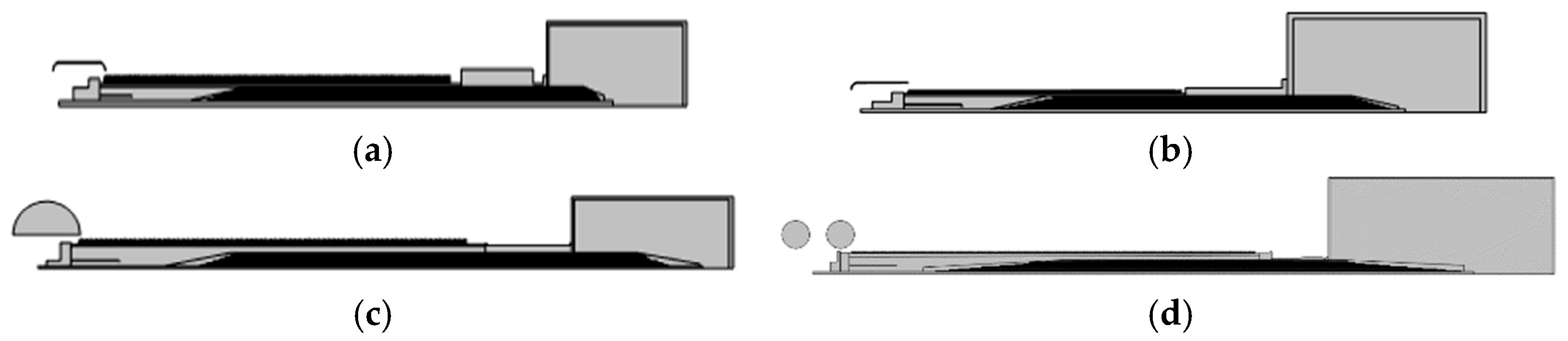
A conducted comprehensive tests across three scenarios are built to evaluate the robustness of SN-POD: spatial resolution variations (assess the ROM accuracy across different FOM meshes), temporal sampling variations (verify performance consistency with varying snapshot quantities), and excitation variations (test parametric generalization).

The average error between the SN-POD ROM and the FOM is around 0.97% under the basic condition, with minimal fluctuations under varying voltage conditions, as in Figure 16b–f, showing that the average error decreases to 0.78% with mesh refinement and increases to 1.36% with mesh coarsening. When the number of snapshots is increased, the average error further reduces to 0.72%, while it rises to 2.37% with fewer snapshots, as in Figure 16g,f.

These results demonstrate that SN-POD maintains strong robustness across diverse scenarios and is highly effective for analyzing the complex physical fields of bushings. However, it is relatively sensitive to temporal sampling, highlighting the need for a careful consideration of snapshot selection in its application. Additionally, the error comparison under the reduced retention mode is included in Figure 16i. It is found that when the number of retained modes is reduced, the average error increases significantly to 7.38%, indicating that the main source of error is the truncation of the order of retained modes.

4.2. The Impact of Order Mode and Sample Time

After performing the dimensionality reduction using the SN-POD, the eigenvalues are arranged in descending order. The larger the eigenvalue is, the greater the proportion of the ability to reflect the physical quantity characteristics it has. During the reduction process, multiple modal diagrams are generated. Modes with higher energy contain more information about the results. Taking the temperature field under normal operating conditions as an example, the first-order and second-order modes are shown in Figure 17.

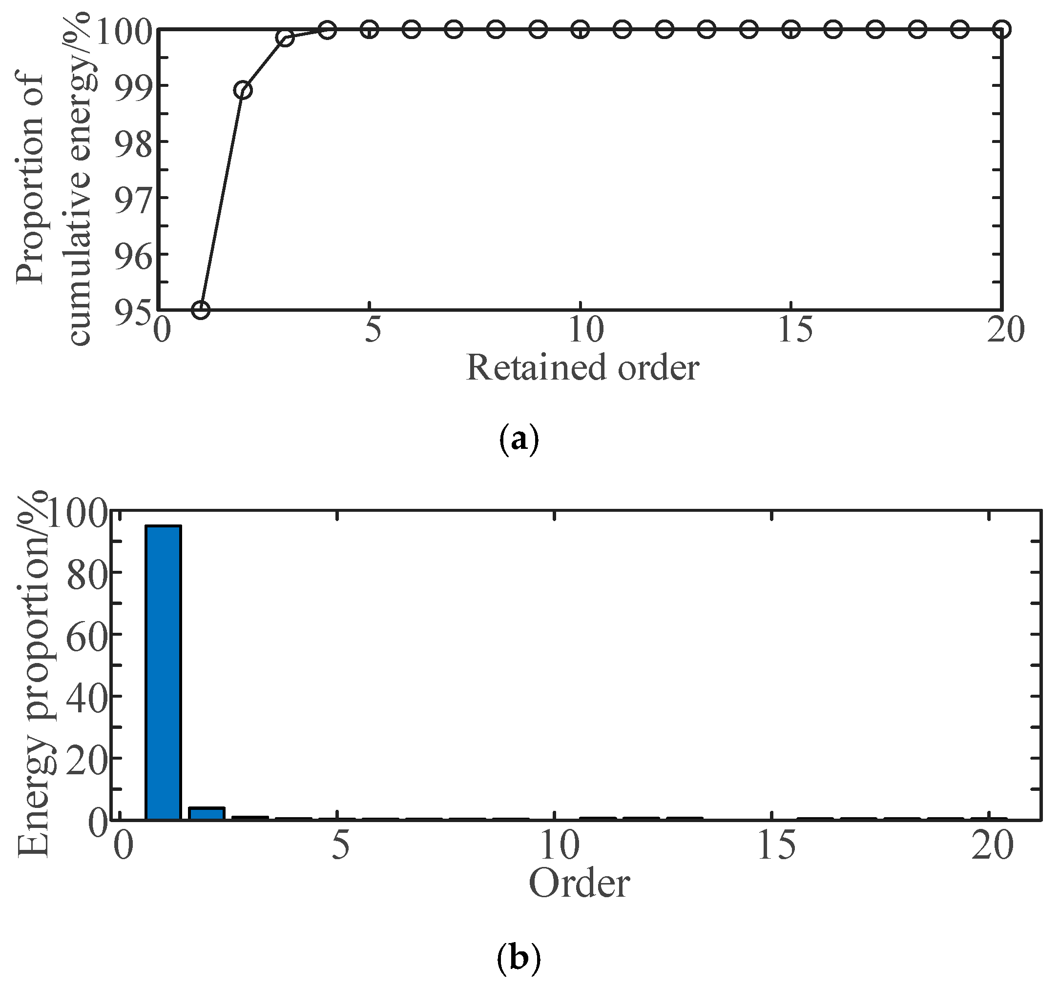
The first-order mode has the highest energy proportion but cannot fully represent all physical variations. Therefore, the number of modes to be included is typically determined based on a predefined error range, following the principle of selecting modes in descending order of energy. Figure 18a shows the energy corresponding to each mode in descending order under normal AC excitation. It is evident that the energy of the first-order mode is significantly higher than that of the other modes. Figure 18b illustrates the accuracy variations when different numbers of modes are combined. It can be preliminarily concluded that the first five eigenvalues capture most of the system’s information. When retaining five modes, the error between the ROM and the FOM is less than 0.01%, indicating that the ROM effectively approximates the FOM.

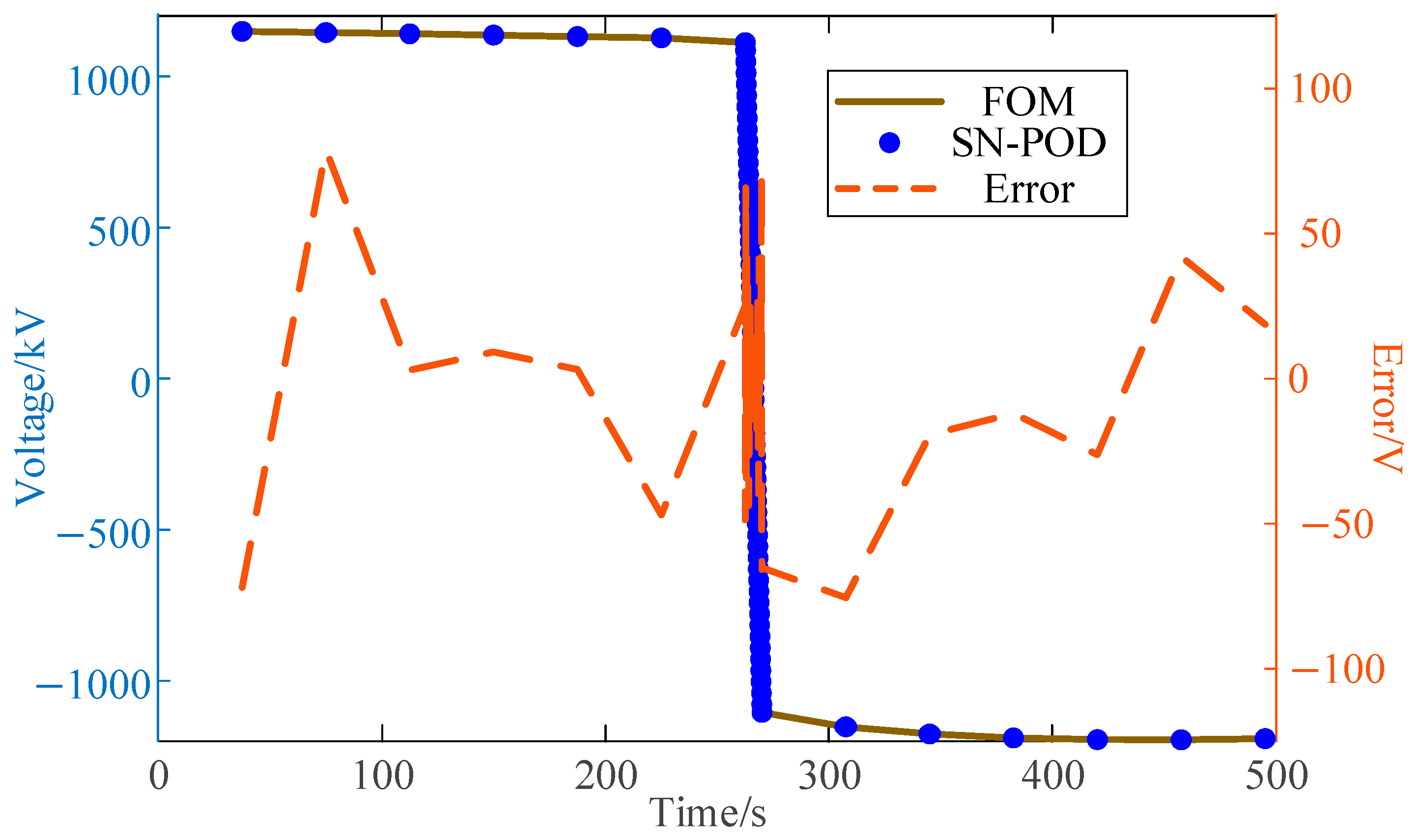
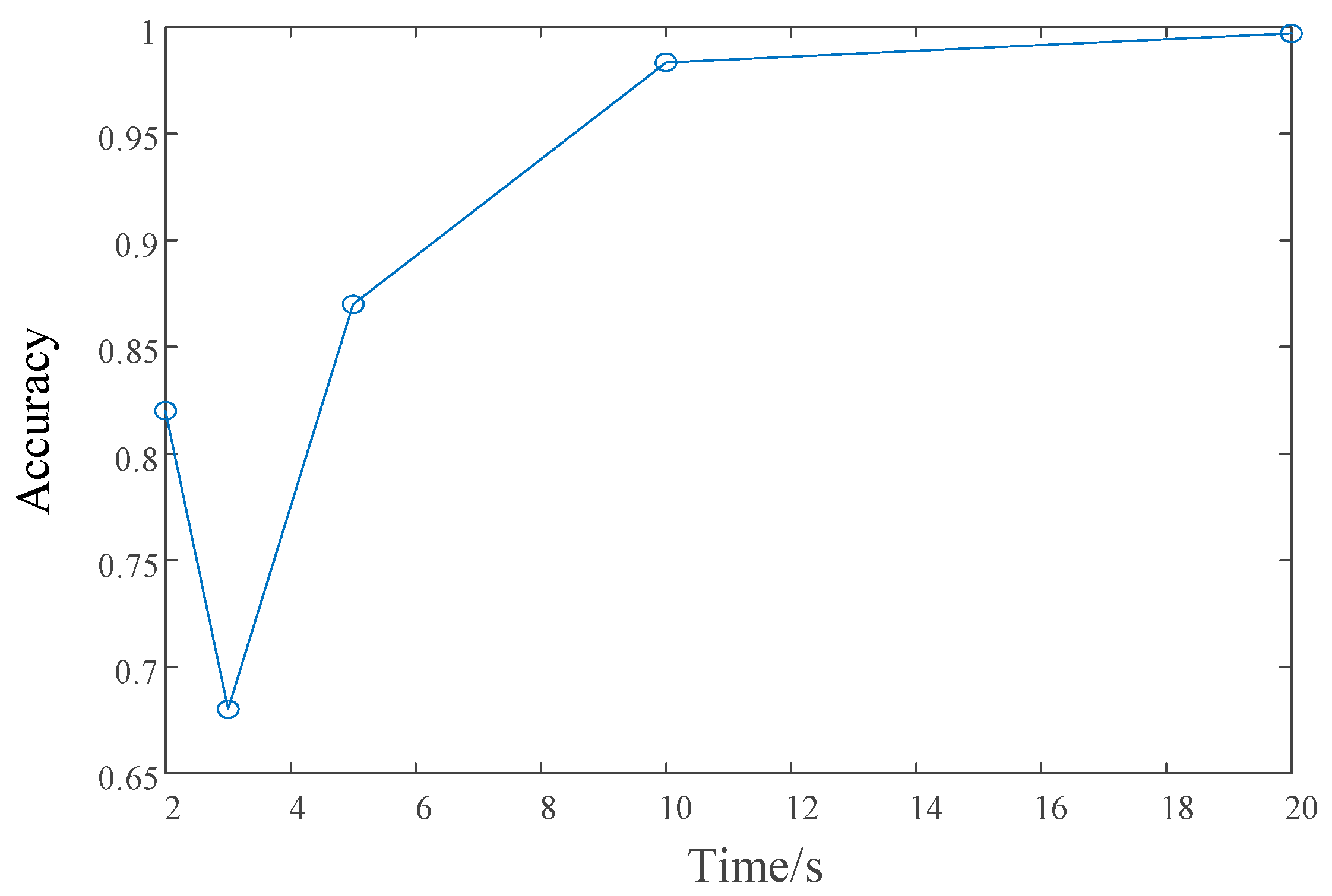
Figure 19 analyzes the impact of the sampling time (sample size) on the relative error, using the case where the excitation is added at 2.5 s as an example. By controlling variables, the analysis uses the accuracy of the three-mode approximation while varying the sampling durations: 2 s, 3 s, 5 s, 10 s, and 20 s. Compared to the FOM, the accuracy of the reduced-order results for these sampling durations is 82.3%, 68.6%, 87.4%, 98.3%, and 99.695%. Since the excitation occurs at 2.5 s, a sudden drop in accuracy is observed when the sampling duration is between 2 s and 3 s. However, as the sampling time increases, the accuracy improves steadily until it stabilizes after 12 s of sampling. The above analysis shows that the accuracy and error of the reduced-order results are influenced by the timing of excitation, the sampling moments, and the sampling duration. In this example, the further the sampling duration extends beyond 2.5 s and the more data are collected, the higher the accuracy and the smaller the error.

It is worth noting that, during the application of the SN-POD method, if computational resources allow, more modes can be retained to meet high-precision reduction requirements (0.01% as used in this study, or even higher). Conversely, when computational resources are highly constrained, the relationship between accuracy and the number of retained modes analyzed in this section can be used to make reasonable choices regarding the number of modes. This ensures a proper balance between the computational accuracy and time efficiency of the valve-side bushing digital twin model.

4.3. The Impact of Different Voltage Levels

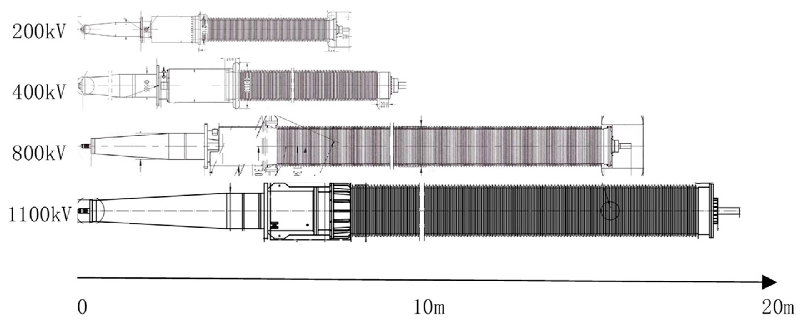
The structures of valve-side bushings used at different voltage levels are shown in the Figure 20. It is evident that the bushings used for ultra-high-voltage (UHV) systems (e.g., 800 kV) are significantly larger than those commonly used in systems below 500 kV. This size increase results in a much more complex model when constructing the bushing for UHV applications.

Taking valve-side bushings for converter transformers at different voltage levels as examples, the modeling parameters are presented in the

Table 2. Model-related information.

Voltage	Length (m)	Number of Nodes	Single Grid Area	Model Size (MB)
200 kV	8	29,065	0.345 × 10−7	65.6
400 kV	9	18,946	0.836 × 10−7	212.6
800 kV	16	21,315	1.525 × 10−7	325.6
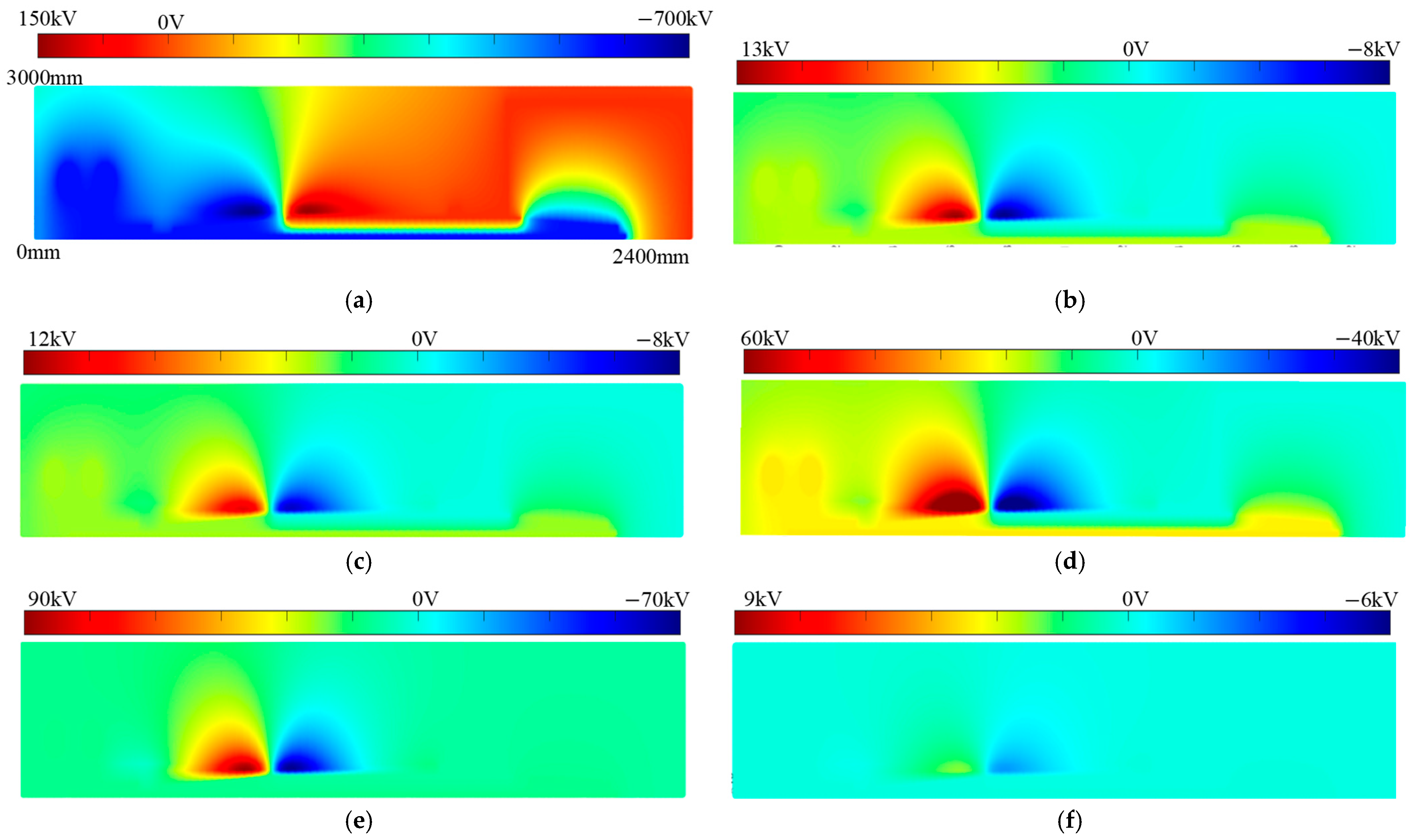
1100 kV	19	25,236	2.815 × 10−7	509.5

. This table shows that the modeling complexity of UHV valve-side bushings is significantly higher than that of lower voltage levels, which, in turn, leads to more intricate models and larger computational demands. This paper conducts full-order and reduced-order calculations for valve-side bushings under polarity reversal conditions at different voltage levels, as shown in Figure 21.

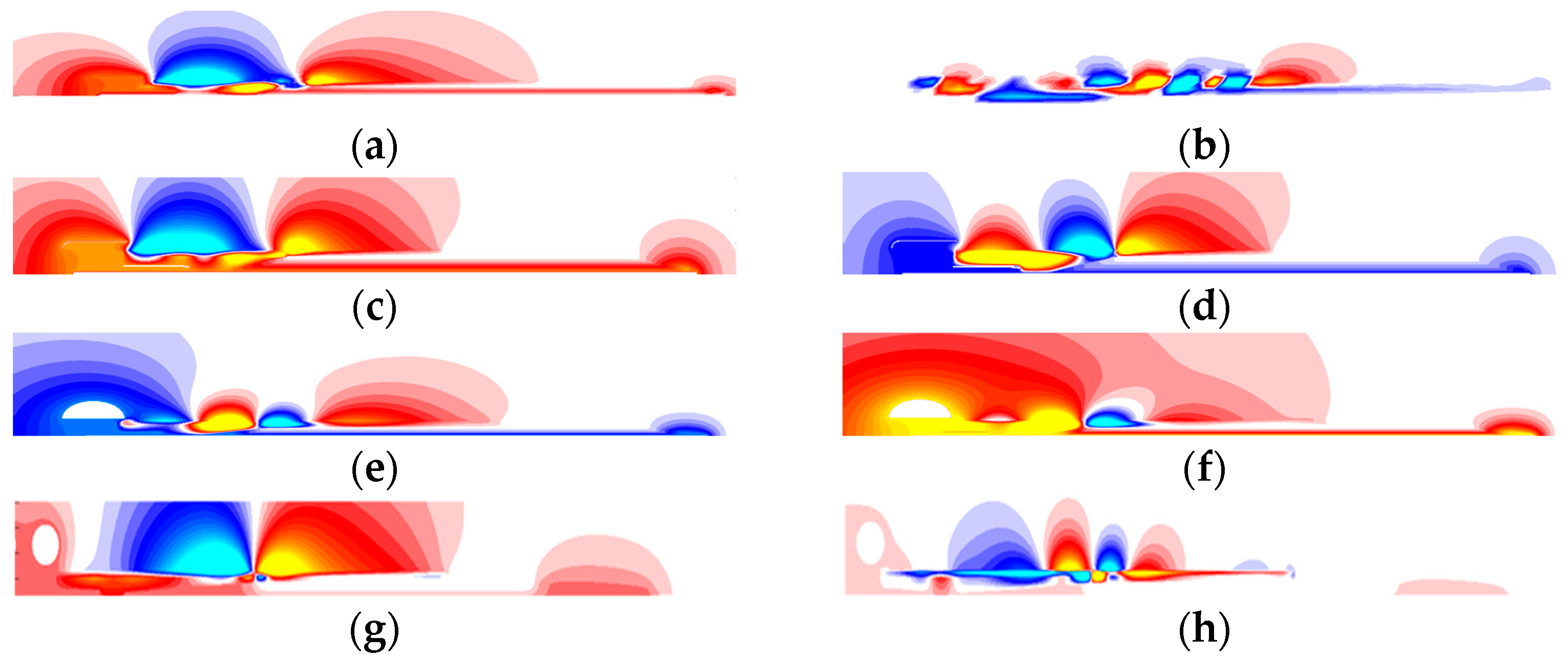
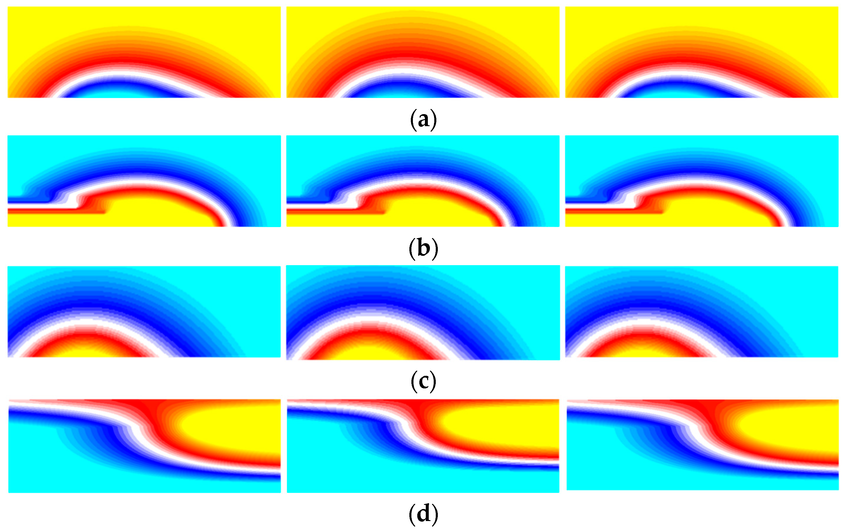
Figure 22 presents the modal decomposition results of the FOM for valve-side bushings at different voltage levels, with a focus on the distribution of the first and second modes. Figure 23 shows the full-order results, reduced-order results retaining only the first mode, and reduced-order results with a maximum error of 0.1% for specific regions of the bushings at various voltage levels. As can be seen from these figures, the higher-order modes can still effectively preserve the features of the model while maintaining a sufficient error (0.1%).

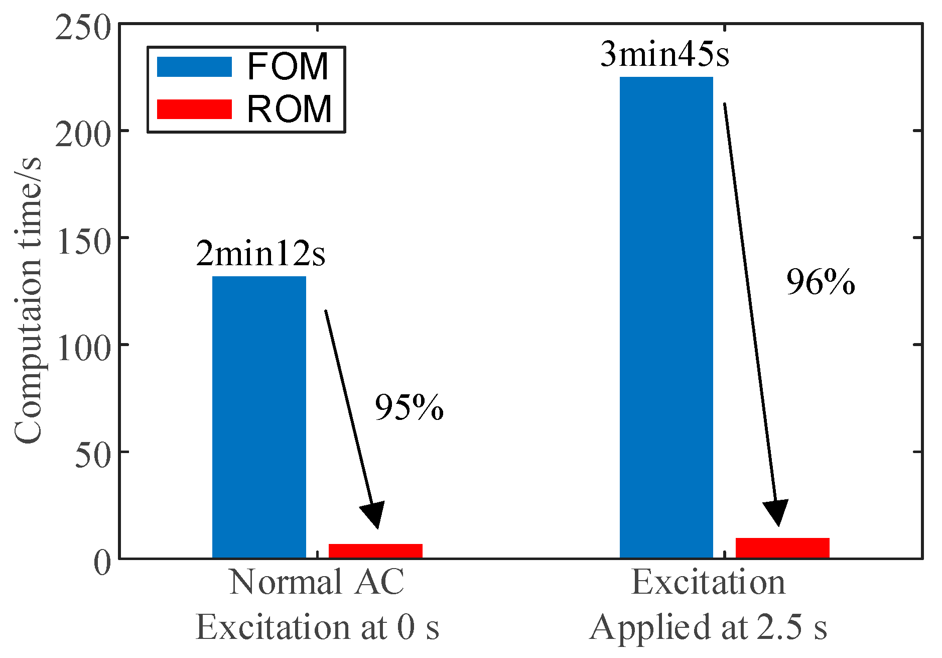
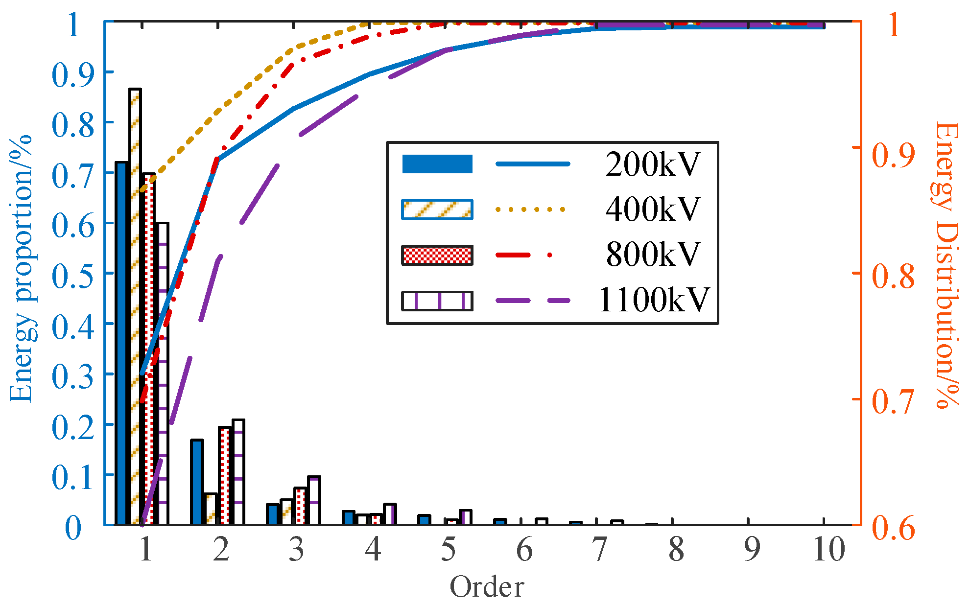
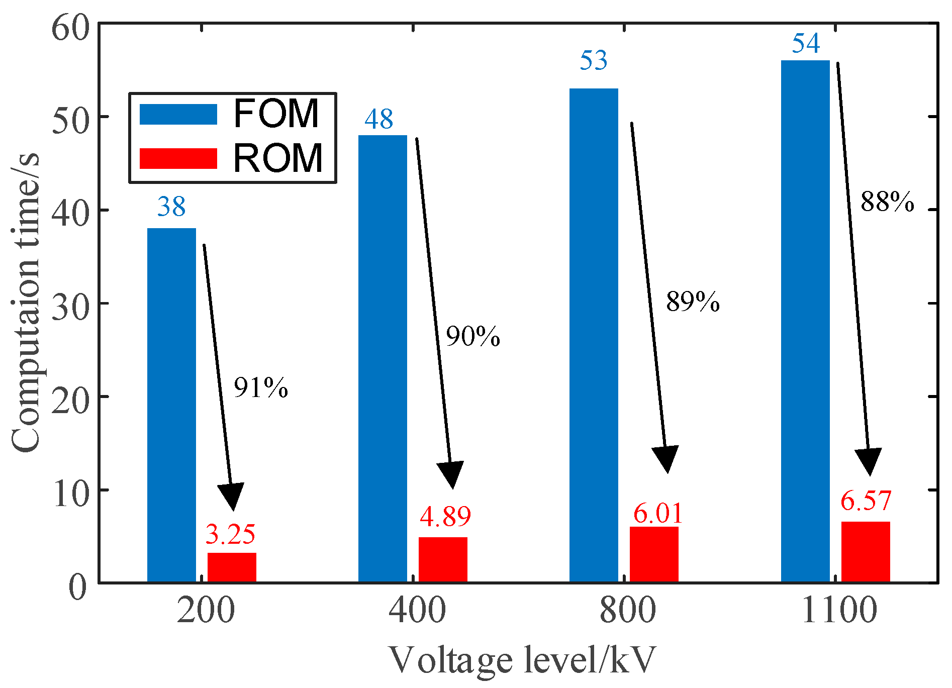
Figure 24 shows the energy at each stage of bushing with different voltage levels. The higher-order results need to be retained to ensure the accuracy of the ROM with the increase in the voltage level. The comparison of the computation time before and after the reduction is shown in Figure 25. It is evident that valve-side bushings at higher voltage levels require longer computation times, making the advantages of the reduced-order approach more apparent.

4.4. Comparison of Different Reduced-Order Algorithms

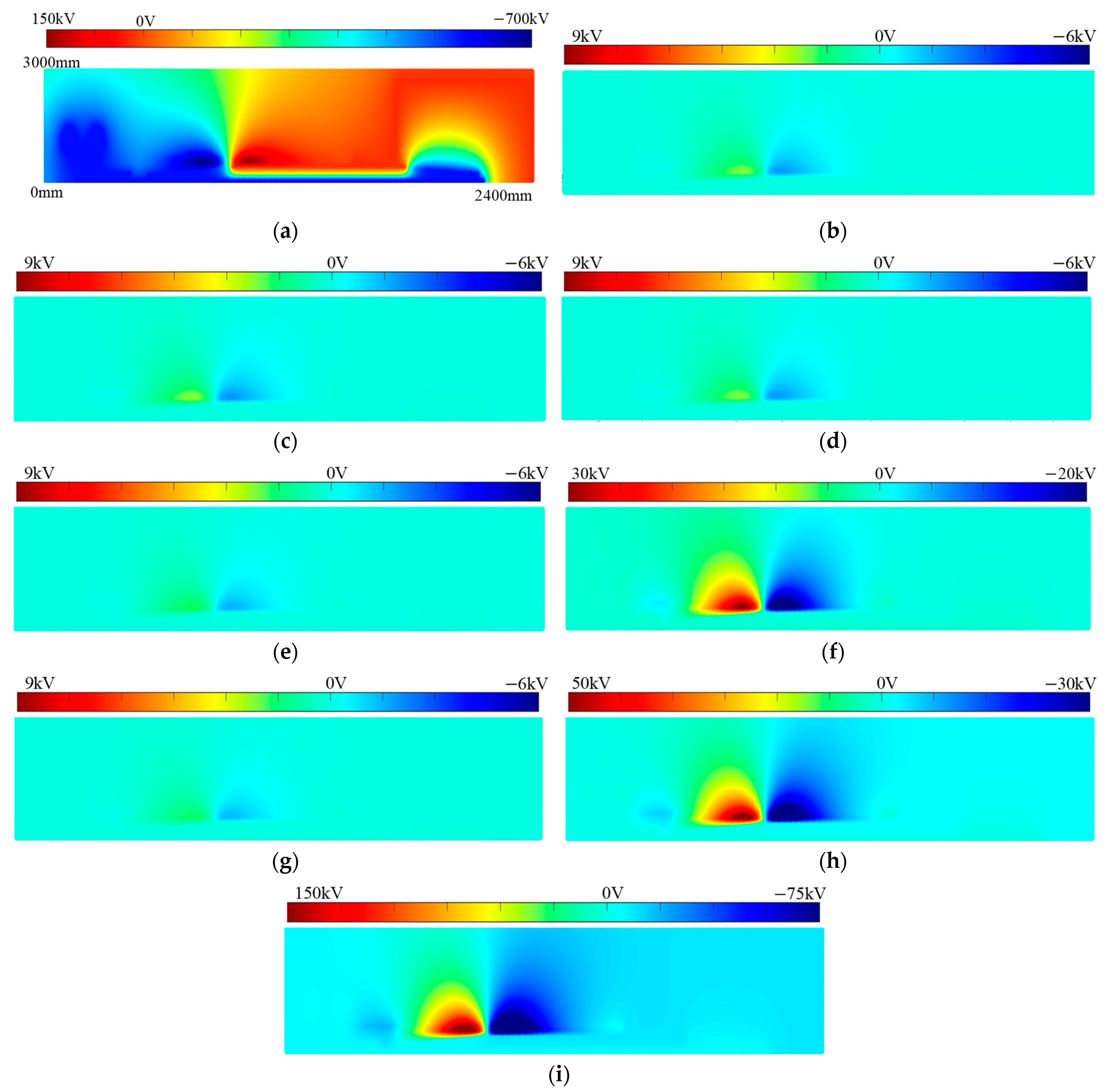
Several methods are compared under the same working conditions in Figure 26. Figure 26a presents the simulation results of the FOM under the given conditions, while the subsequent figures illustrate the error characteristics of different reduced-order methods relative to this reference. The POD exhibits an average relative error of 0.73% with a maximum error of 0.95% in Figure 26b. The adaptive time-stepping method demonstrates higher accuracy in Figure 26c, with an average error of 0.57% and a maximum error of 0.64%. In contrast, the DMD shows significantly larger deviations, with an average error of 4.26% and a maximum error of 5.02% in Figure 26c. SP-POD achieves an intermediate performance, with an average error of 3.07% and a maximum error of 3.32% in Figure 26d. Notably, the SN-POD method outperforms all other methods, achieving a maximum error of only 0.1% and an average error of 0.097% in Figure 26e. Furthermore, the SN-POD method demonstrates an exceptional performance in the internal errors of the casing, with errors of 0.053% for the capacitor core, 0.025% for the conductive rod, and 0.039% for the flange.

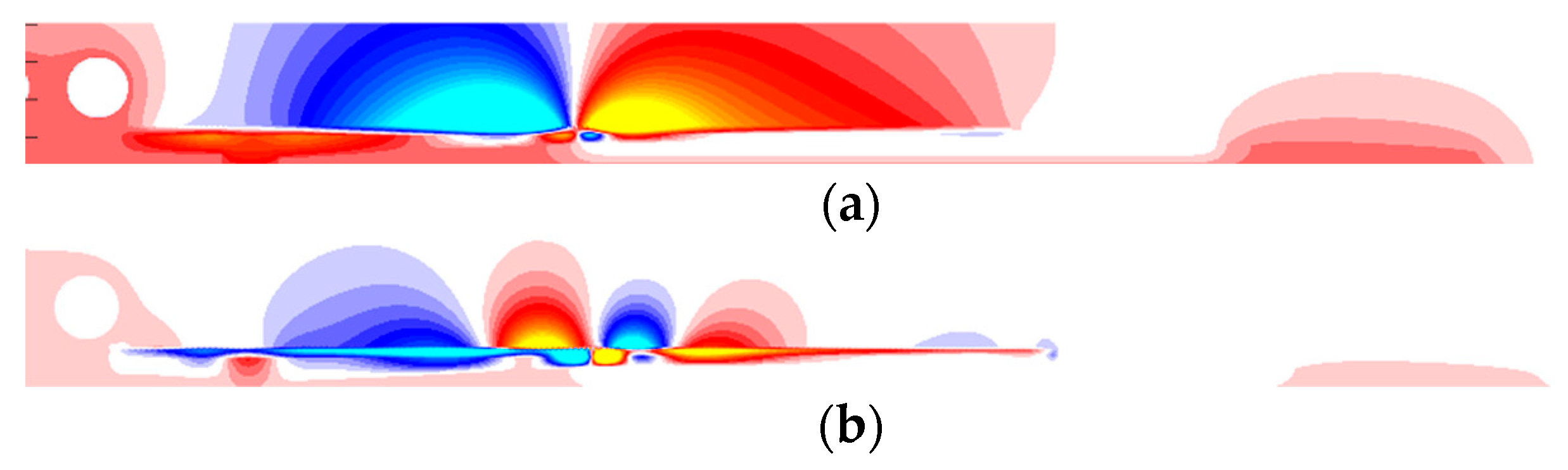
It is noteworthy that the error distribution exhibits significant regional characteristics compared to other algorithms: traditional methods primarily accumulate errors in both the capacitive core region inside the bushing and the external area of the bushing, whereas the SP-POD and SN-POD methods, due to their focused sampling strategy in critical internal regions, demonstrate predominant errors in the external area of the bushing. Furthermore, a comparative analysis reveals that the SN-POD method achieves significantly lower errors than SP-POD. This enhanced performance can be attributed to the temporal sampling refinement employed in SN-POD, which not only focuses on spatial optimization but also increases the density of time sampling. This dual refinement strategy enables SN-POD to capture dynamic behaviors more accurately, thereby achieving a superior performance in the rapid and precise analysis of the bushing and laying a solid foundation for constructing a digital twin model of the bushing.

The comparison of different reduced-order algorithms applied to the calculation of bushing digital twins is shown in

Table 3. Comparison of computing efficiency between SVD-POD and spatial non-uniformity POD.

	Calculation Time	Improvement	Maximum Calculation Error
FOM	54 s	-	-
POD [9,10,11,12]	11.57 s	79%	0.95%
Adaptive steps [13,15]	19.87 s	63%	0.64%
DMD [7,8]	4.3856 s	92%	5.02%
SP-POD [24]	14.86 s	73%	3.32%
SN-POD	6.57 s	88%	0.1%

. All the algorithms can improve the computing efficiency compared with the FOM, and SN-POD achieves a significant increase of 88% with a small calculation error of 0.1%.

Although the calculation efficiency of SN-POD (88%) is lower than DMD (92%), its calculation error (0.1%) is far lower than DMD (5%). Due to the sensitivity of DMD to noise in the data, which makes it highly dependent on the quality of the data, it can easily amplify errors after order reduction. SN-POD requires the construction of reduced-order finite element equations and recalculations, which allows it to retain the physical characteristics of the system to a certain extent and accurately capture the dominant modes of the system with a small calculation error.

Although it should be noted that the online computation phase remains constrained by the intrinsic framework of the POD theory, due to the need for iterative mode construction, eigenvalue decomposition, and reduced-order finite element calculations, SN-POD achieves an effective balance between reducing the model complexity and preserving high precision, laying the theoretical foundation for constructing digital twin systems for complex electrical equipment.

Future research could focus on integrating it with other rapid computation methodologies while retaining its data compression advantages, thereby further improving the real-time computational performance.

5. Conclusions

In this paper, a reduced-order algorithm for digital twins is proposed by incorporating the importance of different regions and the temporal variations in physical quantities. The main conclusions are as follows:

• The computation time of SN-POD is reduced by nearly 95% compared to the FOM and by approximately 40% compared to SVD-POD, by ensuring that the reduced-order results for critical regions of the valve-side bushing have an error within 0.1%. The proposed method significantly reduces the runtime of the model for valve-side bushing reduction.
• As the structure of valve-side bushings becomes increasingly complex with higher voltage levels, resulting in larger computational workloads, the proposed method effectively reduces the computation time for ultra-high-voltage valve-side bushings, maintaining it within the second scale. This method can also demonstrate good robustness in different running environments. Compared with other methods, the proposed method can improve the computational efficiency of large-scale problems and maintain a good calculation error.

This proposed method developed in this study, tailored to the unique structure of valve-side bushings, enables more efficient and faster multi-physical field computations, which could provide algorithmic support for applying digital twin models of valve-side bushings in monitoring and early warning systems.