Article

Using CPC-Based Minimizing Balancing Compensation to Reduce the Budeanu Reactive Currents Described in Extended Budeanu Theory

Faculty of Electrical Engineering, Bialystok University of Technology, Wiejska 45D Street, 15-351 Białystok, Poland
Energies 2025, 18(6), 1476; https://doi.org/10.3390/en18061476
Submission received: 16 February 2025 / Revised: 12 March 2025 / Accepted: 14 March 2025 / Published: 17 March 2025
(This article belongs to the Section F: Electrical Engineering)

Abstract

:
This article presents principles for matching reactance parameters for minimizing balancing compensation, whose mathematical origins come from the Currents’ Physical Components (CPC) theory developed by Czarnecki. The construction of minimizing balancing compensators was considered by applying it to the concept of the extended Budeanu theory. It focuses on the possibility of compensating the Budeanu reactive current, Budeanu complemented reactive current, and both currents at the same time. In addition, the compensator also has the potential to balance the load, that is, to reduce the unbalanced current. In order to precisely illustrate the difference in the effectiveness of compensation and balancing the load, each approach to minimizing balancing compensation has its equivalent in the case of ideal compensation. The analysis of the results achieved is a comparison of the three-phase RMS values of the respective components and the current of the load at the primary load and using three approaches, with each approach divided into ideal compensation and minimizing balancing compensation. For all approaches, calculations and simulations were carried out, in which the numerical values and generated waveforms of each quantity were compiled and analyzed. The Matlab/Simulink R2023a application environment was used as computational and simulation software.

1. Introduction

The first power theories appeared to take form in the 1920s and 1930s, distinguishing two main trends. The first is based on a Fourier series [1,2,3,4,5,6], describing the energy properties of a circuit in the frequency domain by decomposing electrical waveforms into components at different frequencies. Almost in parallel, a second trend was formed, which defines energy quantities, without the use of a Fourier series, as time functions of current and voltage in the time domain [7,8,9,10,11].
The problem of the inexistence of a unified and globally accepted theory describing the energy properties of circuits with nonsinusoidal waveforms is intensified with the invention of semiconductor elements and the evolution of power electronics. Although power electronic systems have numerous advantages, they also generate negative phenomena. The increase in the number of nonlinear power electronic loads has caused a significant expansion of the quantity of higher harmonics, which negatively affects the power grid, for example, an increase in the asymmetry of supply voltage [12] transfer of capacitive reactive energy into the grid, which leads to a rise in the voltage value [13], an increase in the asymmetry of currents flowing through the network, an increase in the asymmetry of the zero sequence [14], disturbances in wireless energy transmission resulting from the commutation operation of converters [15], disturbances in the stability of the electromagnetic field [16], distortions in supply voltages in lighting circuits [17], power oscillations appearing after a disturbance caused by the lack of inertia and damping of the converter [18], a rise in power and energy losses [19], an impact on active power circulation caused by the difference in parameters between different types of generation units [20], and an increase in distortion related to higher harmonics [21].
Since the 1970s, there has been expanding interest in describing the energy properties of these devices and in methods of optimizing the power factor [22,23,24,25,26,27]. Currently, there are many concepts for studying electrical systems under distorted voltage and current waveforms. The proposed power theories are subject to debates and do not always obtain widespread acceptance.
For many decades, one of the dominant power theories was the Budeanu concept [2]. However, as Czarnecki [28] has shown, this theory is flawed. Despite the errors in this theory, it is still the main concept presented to young students of electrical engineering. An important contribution to the progress of power theory was also made by Fryze’s proposal [7], which still plays a significant role.
Currently, one of the most widely used theories (according to the author of the publication, the p-q method is a control algorithm and not a power theory—however, this is beyond the scope of this manuscript), especially in the field of active filtering, is the p-q power theory proposed by Akagi’s team [8,9] and power theory concepts related to the original p-q method along with positive [9,29,30,31] as well as negative aspects, where the main objection is the increase in the third harmonic current and its injection into the compensator current and the load current [32,33,34,35]. Nevertheless, in the opinion of many experts, the most correct interpretation of the energy properties of electrical systems and a powerful mathematical instrument is offered by the power theory based on the concept of Currents’ Physical Components, formulated by Czarnecki [3].
With the CPC power theory, it is possible to apply a minimizing balancing compensation method [36,37,38], which is used in this article. It is based on the combination of reactance parameters that minimize the reactive component of the load’s current and minimize and balance the three components of unbalance, i.e., the unbalanced current of the positive sequence, the unbalanced current of the negative sequence, and the unbalanced current of the zero sequence. Such a system is less sensitive to changes in the current–voltage conditions in the circuit and is more suitable as a passive component in hybrid filters [23,39,40,41].
Extended Budeanu theory is the most recognized and most frequently applied concept of power theory in the electrical power industry and in electrical engineering programs. However, it did not have a sufficiently clear mathematical description, especially because of the problem with the components of distortion power. The problem of the description and identification of physical phenomena has been discussed in a study [4]. The next step in the improvement in Budeanu’s power theory was to demonstrate the potential for the optimal compensation of individual components of the current [27], as described in this publication in a minimized way. It is based on modifying selected components in a way that minimizes the need for full compensation, while reducing dependence on the power supply and load conditions. Moreover, it is important to consider the economic parameter of applying a minimizing balancing compensator, i.e., the lower cost of elements necessary to construct the compensator.
This article is organized into 13 sections. Section 1 describes the differences between power theories and algorithms used to control frequency converters and the possibility of using passive configurations in the power network. Section 2 is dedicated to a brief characterization of extended Budeanu theory. Section 3 presents a theoretical illustration 1 based on calculations and simulations of a 3-phase 4-wire load following extended Budeanu theory. Section 4 explains the ideal compensation approach, which is explained in detail in [27]. Section 5 is about minimizing balancing compensation, which is inspired by Currents’ Physical Components theory. Section 6 and Section 7 presents calculations and simulations of the ideal compensator and the minimizing balancing compensator for the Budeanu complemented reactive current, which was attached to the load described in Section 4. Similarly, Section 8 and Section 9 refer to the calculations and simulations of the compensators in relation to a reduction in the Budeanu reactive current. Section 10 and Section 11 describe a complex approach to compensation, i.e., the consideration of both Budeanu currents in calculations and simulations, namely, the Budeanu complemented reactive current and the Budeanu reactive current, which together form the Czarnecki’s reactive current. Section 12 presents an analysis of the results obtained with respect to the three-phase RMS values of the load current components and the power factor after compensation as well as a brief economic analysis of the costs of the reactance components needed to build the compensators. This study is summarized in Section 13, which presents the conclusions resulting from the theoretical components and the research results.

2. Description of the Load’s Currents in Extended Budeanu Theory for 3-Phase 4-Wire Systems

For the exact derivation of the formulas and a detailed description of extended Budeanu theory, see [4]. The basis for the energy description in extended Budeanu theory is the concept of power theory proposed by Czarnecki—Currents’ Physical Components theory [5].
The circuit shown in Figure 1 is a three-phase four-wire system in which the voltage vector is symmetric and also has higher-order harmonics.
The vector of fundamental and higher-order harmonic voltages is expressed by the following equation [5]:
u ( t ) = [ u R ( t ) u S ( t ) u T ( t ) ] = 2 Re n N [ U R n U S n U T n ] e j n ω 1 t = 2 Re n N U n e j n ω 1 t
where U n is the vector of the CRMS (complex RMS) value of the voltage harmonics and n is the harmonic order.
When a linear load is connected to the power supply, currents that correlate with the supply voltage vector are obtained:
i ( t ) = [ i R ( t ) i S ( t ) i T ( t ) ] = 2 Re n N [ I R n I S n I T n ] e j n ω 1 t = 2 Re n N I n e j n ω 1 t
where I n is the vector of CRMS (complex RMS) value of the current harmonics.
Following [4], the current of a load in a three-phase four-wire system with distorted waveforms can have 7 mutually orthogonal components. Each of the components can be defined in the time waveform or a three-phase RMS value. In addition, each of the currents, in combination with the voltage, results in the appropriate power. Table 1 summarizes the current components and power of a linear load as given in the extended Budeanu theory.
All the current components of the load and the power components of the load form the entire current’s value i :
i 2 = i a 2 + i s 2 + i rB 2 + i crB 2 + i u p 2 + i u n 2 + i u z 2
and three-phase apparent power S is as follows:
S = u i
The λ power factor of a system described in the extended Budeanu theory is adequately expressed in the CPC theory, i.e., it can be described using the component powers:
λ = P S = P P 2 + D s 2 + Q B 2 + Q crB 2 + D u p 2 + D u n 2 + D u z 2
or the currents’ components:
λ = i a i = i a i a 2 + i s 2 + i B 2 + i crB 2 + i u p 2 + i u n 2 + i u z 2
To find the parameters of the Budeanu compensator for minimizing the Budeanu reactive current and/or the Budeanu complemented reactive current, the components of the current of the load have to be determined, as presented above. The specification of the parameters of a minimizing balancing compensator can be achieved in three steps, namely:
  • Step 1—the determination of equivalent parameters and load currents.
  • Step 2—the determination of the parameters of an ideal compensator based on the equivalent parameters of the load.
  • Step 3—the determination of the parameters of the minimizing balancing compensator based on the parameters of the ideal compensator and the equivalent parameters of the load.
It can be seen that none of the steps can be ignored because they are all mutually connected.

3. Theoretical Illustration 1—Original System with Three-Phase Four-Wire Linear Load

The electrical circuit in Figure 1 is powered by a symmetric nonsinusoidal voltage waveform. In addition to the fundamental harmonic, the source of nonsinusoidal voltage also produces higher-order harmonics, i.e., n = 3, 5, and 7, which form a symmetrical waveform in each phase in the following form: u ( t ) = { 230 e j ω t + 5 e j 3 ω t + 30 e j 5 ω t + 5 e j 7 ω t }    V . The frequency of the primary harmonic n 1 is 50 Hz. A three-phase load has linear elements in the components of resistance, inductive reactance, and capacitive reactance, with a load asymmetry. The electrical circuit is visualized in Figure 2.
Figure 3 shows the waveform of the supply voltage at connections points R, S, T of an imbalanced linear load.
The three-phase RMS value of the discussed voltage is as follows:
u = 401.93    V
The receiver in Figure 3 consists of the elements R, L, and C. The resistance, inductive reactance, and capacitive reactance values for fundamental frequency are compiled in Table 2.
Using the data presented in Table 2 and the details regarding the supply voltage, the line currents for each harmonic were obtained. The resulting current waveform of the analyzed load is shown in Figure 4.
The three-phase RMS value of the load current, the waveform of which is shown in Figure 4, is as follows (3):
i = 76.918    A
Based on the information in [2,4,5] regarding Budeanu’s power theory [2] and extended Budeanu theory [4], the active powers P and reactive Budeanu powers QB are summarized in Table 3. Based on extended Budeanu theory, the powers of the specific harmonics were summed up, even though the powers of the respective harmonic are capacitive or inductive.
The apparent power S is as follows (4):
S = 30 , 916    VA
and the Budeanu distortion power DB [2,4] is as follows:
D B = 18 , 239.5    VA
According to the publication [4], the components of the load current described in the extended Budeanu theory are summarized in Table 4.
The three-phase RMS value in the extended Budeanu theory is i = 76.918    A .
In the case under study, 5 components of the current are responsible for the Budeanu distortion current. The waveform of the Budeanu distortion current described in the extended Budeanu theory is shown in Figure 5.
Table 5 summarizes the three-phase RMS values of the components of the currents, which can be used to determine the distortion current and, thus, the distortion power described by Budeanu.
Based on Equation (6), the power factor λ is as follows:
λ = 0.766
This requires that the receiver in Figure 2 follows the ideal compensation or minimization of the balancing compensation in order to achieve the highest possible power factor.

4. Optimal Compensation of the Budeanu Complemented Reactive Current and the Unbalanced Current

The increase in the power factor through ideal compensation is described in [27]. At this point, it should be emphasized that the calculated parameters of an ideal compensator, as the name suggests, are lossless and do not cause any other interferences (e.g., no additional resistance). This means that after finding the parameters of the reactance elements, connecting them in the required configuration, and tuning them to a given harmonic, they do not influence the current value of the rest of the harmonics.
The formulas that make this possible are demonstrated below. Extended Budeanu theory describes two reactive components of the load current, namely, the Budeanu reactive current and the Budeanu complemented reactive current. It should be pointed out, however, that after summing up both reactive currents, the reactive current described by Czarnecki in Currents’ Physical Components theory is formed. Considering the above conclusions and the basic idea in [22], the result of the two expressions concerning the compensation of the chosen reactive current component and the unbalanced current of the zero sequence for the sequence of harmonics n = 3 k + 1 is as follows:
T R n = 2 Im Y u n z ( M x ) T S n = 3 Re Y u n z + Im Y u n z ( M x ) T T n = 3 Re Y u n z + Im Y u n z ( M x )
where the parameter M x can be described as follows, respectively:
1.
M x = ( B n B e ) —Budeanu complemented reactive current compensation.
2.
M x = B e —Budeanu reactive current compensation.
3.
M x = [ ( B n B e ) + B e ] —Budeanu complemented reactive current and Budeanu reactive current compensations, i.e., the Czarnecki reactive current.
For the positive sequence n = 3 k + 1, a delta-structure compensator is described by the following group of equations:
T RS n = 1 3 ( 3 Re Y u n n # Im Y u n n # ) T ST n = 1 3 ( 2 Im Y u n n # ) T TR n = 1 3 ( 3 Re Y u n n # Im Y u n n # )
If the supply voltage has negative-sequence harmonics n = 3 k − 1, then, the answer to Equation (7) is as follows:
T R n = 2 Im Y u n z ( M x ) T S n = 3 Re Y u n z + Im Y u n z ( M x ) T T n = 3 Re Y u n z + Im Y u n z ( M x )
Then, the solution of Equation (8) changes. For the negative-sequence harmonics n = 3 k − 1, it is as follows:
T RS n = 1 3 ( 3 Re Y u n p # Im Y u n p # ) T ST n = 1 3 ( 2 Im Y u n p # ) T TR n = 1 3 ( 3 Re Y u n p # Im Y u n p # )
For zero-sequence voltage harmonics n = 3 k, only the configuration of a star-structure compensator can be used. When choosing the compensation for the positive-sequence unbalanced current, the solution to the equation is as follows:
T R n = 2 Im Y u n p ( M x ) T S n = 3 Re Y u n p + Im Y u n p ( M x ) T T n = 3 Re Y u n p + Im Y u n p ( M x )
If the unbalanced current of the negative sequence is chosen for compensation, the equation has the following solution:
T R n = 2 Im Y u n n ( M x ) T S n = 3 Re Y u n n + Im Y u n n ( M x ) T T n = 3 Re Y u n n + Im Y u n n ( M x )
In this article, the unbalanced component of the current of the positive sequence was taken into account when setting the parameters of the compensator for harmonics n = 3 k.

5. Minimizing Balancing Compensation in Extended Budeanu Theory

It is clear that the RMS value of the first voltage harmonic, whether phase-to-phase or phase, is significantly higher than the RMS value of any additional harmonic [36,37,38].
The principle is that if the susceptance TXY1 or TX1 is negative, the delta-structure compensator between the TXY connection points may have an electrical line with a choke as its susceptance is also below zero, or for the star-structure compensator between the phase connection point and the neutral connection point with susceptance TX, it should also have a branch with a choke. The inductance of that choke, regardless of whether it is connected between the phases or between the phase and the neutral point, should minimize the value [36,37,38]:
n N ( T k n + 1 n ω 1 L k ) 2 U k n 2 = minimum
If the phase-to-phase TXY or phase TX susceptance has a “plus” sign, the compensator may have a capacitor in the electrical line, but it needs to be put together in series with an inductor; so, for harmonic distortion, this electrical line has an inductive character, and for the basic frequency, it is still positive:
d k 1 = ω 1 C k 1 ω 1 2 L k C k
This demands that the resonant frequency of that branch is higher than the fundamental harmonic frequency, as follows:
ω r = 1 L k C k
The inductance and capacitance of such a branch should follow to minimize the expression below:
n N ( T k n n ω 1 C k 1 n 2 ω 1 2 L k C k ) 2 U k n 2 = minimum
Inductance L k fulfills Equation (15) and can be obtained as follows:
d d L k { n N ( T k n + 1 n ω 1 L k ) 2 U k n 2 } = 0
By satisfying expression (17), i.e., calculating the inductance in a determined branch in this procedure, we can interpret it as the optimal inductance of this branch, as follows:
L k , opt = n N U k n 2 n 2 ω 1 n N T k n U k n 2 n
The left side of expression (16) represents a function with two parameters, i.e., inductance L k and capacitance C k . Inductance L k is a permanently decreasing function, which means that there is no minimum for any specific value. Its specific choice depends on the person making the calculations [36,37,38]. When the inductance has been determined, the capacitance C k can be found using Equation (16). When solving Equation (16), we must satisfy the following condition:
d d C k { n N ( T k n n ω 1 C k 1 n 2 ω 1 2 L k C k ) 2 U k n 2 } = 0
The distance determined by expression (19) for any branch has a minimum related to the optimal capacitor capacitance when:
n N n T k n U k n 2 ( 1 n 2 ω 1 2 L k , opt C k , opt ) 2 n N n 2 ω 1 C k , opt U k n 2 ( 1 n 2 ω 1 2 L k , opt C k , opt ) 3 = 0
Because of the optimum capacity C k , opt present in expression (20), this is an implicit equation. For this reason, calculating this capacity requires numerical methods, especially in an iterative process. The iterative equation for finding the optimal capacity is as follows:
C k ,    i + 1 = n N n T k n U k n 2 ( 1 n 2 ω 1 2 L k , opt C k ,    i ) 2 ω 1 n N n 2 U k n 2 ( 1 n 2 ω 1 2 L k , opt C k ,    i ) 3
which, after the i-th iteration, will lead to some capacities that should come together to reach the optimal capacity in the final stage of calculations.

6. Theoretical Illustration of the 2-Ideal Compensation of the Budeanu Complemented Reactive Current

The receiver in Figure 2 was connected to the Budeanu complemented reactive current (parameter M x = ( B n B e ) ) and the compensator of the unbalanced current, which is designed to compensate for the susceptances responsible for the Budeanu complemented reactive current for all the harmonics present in the voltage. Moreover, the system is able to balance the load by compensating for the unbalanced current components. Table 6 and Table 7 show the capacitance and inductance values needed to compensate for the Budeanu complemented reactive current and the unbalanced current for the respective harmonics. Figure 6 shows the way in which the discussed compensator is connected (star and delta configurations). Figure 7 shows the waveforms of the line currents obtained by using the Budeanu complemented reactive current and the unbalanced current compensator.
After perfect compensation of the Budeanu complemented reactive current and the unbalanced current, the value of the line current is as follows:
i = 62.195    A
The installation of the Budeanu complemented reactive current and the unbalanced current compensator changes the power values related to passive components. Table 8 summarizes the powers of the individual harmonics and the entire system.
The apparent power S is as follows:
S = 24 , 998.4    VA
and the Budeanu distortion power DB is as follows:
D B = 1340.4    VA
Based on the equations in Table 1, the three-phase RMS values of the currents’ components after the connection of the perfect Budeanu complemented reactive current and the unbalanced current compensator were calculated. The three-phase RMS values of the components of the currents for the individual harmonics described in the extended Budeanu theory are summarized in Table 9.
After perfect compensation of the Budeanu complemented reactive current and the unbalanced current, the value of the line current is i = 62.195    A .
After including the ideal compensator of the Budeanu complemented reactive current and the unbalanced current, the Budeanu distortion current has two components. The waveform of the Budeanu distortion current after the ideal compensation of the Budeanu complemented reactive current and the unbalanced current is shown in Figure 8.
Table 10 summarizes the three-phase RMS values of the currents’ components based on the perfect compensation of the Budeanu complemented reactive current and the unbalanced current, which allow for the description of the Budeanu distortion current.
The power factor of a circuit with an optimally compensated Budeanu complemented reactive current and the unbalanced current is as follows:
λ = 0.947
This means that the receiver in Figure 2, after connecting the optimal compensator of the Budeanu complemented reactive current and the unbalanced current, achieves the highest possible value. In the next section—Section 7, based on the obtained parameters of the ideal compensator, the parameters of the minimizing balancing compensator of the Budeanu complemented reactive current and the unbalanced current are calculated.

7. Theoretical Illustration 3—Minimizing Balancing Compensation of the Budeanu Complemented Reactive Current

A compensator was connected to the receiver in Figure 2, the main function of which is to minimize the 3-phase RMS value of the Budeanu complemented reactive current and the unbalanced current. The design and choice of parameters of the minimizing balancing compensator causes it to impact all components associated with reactance elements. Figure 9 shows how to install the abovementioned compensator. Figure 10 illustrates the current flow of the load caused by the connection of a minimizing balancing compensator.
Table 11 summarizes the inductance and capacitance values obtained from the parameter calculation for a compensator minimizing balancing compensator of the Budeanu complemented reactive current and the unbalanced current.
After the minimizing balancing compensation of the Budeanu complemented reactive current and the unbalanced current, the value of line current is as follows:
i = 62.452    A
Table 12 summarizes the power values of the respective harmonics and the entire system.
The apparent power S is as follows:
S = 25 , 101.5    VA
and the Budeanu distortion power DB is as follows:
D B = 2856.9 VA
Based on the relationships in Table 1, the three-phase RMS values of the currents’ components were calculated after including a minimizing balancing compensator of the Budeanu complemented reactive current and the unbalanced current. The 3-phase RMS values of the load currents for the specific harmonics described in extended Budeanu theory are summarized in Table 13.
The load current after minimizing balancing compensation is i = 62.452    A .
After adding the minimizing balancing compensator of the Budeanu complemented reactive current and the unbalanced current, five currents’ components represent the Budeanu distortion current. The waveform of the Budeanu distortion current after minimizing balancing compensation is given in Figure 11.
Table 14 summarizes the three-phase RMS values of the currents’ components caused by the minimizing balancing compensation of the Budeanu complemented reactive current and the unbalanced current, which describe the distortion current defined by Budeanu.
Power factor λ is equal to:
λ = 0.943
This signifies that the difference between the connection of an ideal compensator to a minimizing balancing compensator of the Budeanu complemented reactive current and the unbalanced current is only 0.004.

8. Theoretical Illustration 4—Ideal Compensation of the Budeanu Reactive Current

The receiver in Figure 2 was connected to the Budeanu reactive current (parameter M x = B e ) and the unbalanced current compensator, which is designed to compensate for the susceptances responsible for the Budeanu reactive current for all the harmonics present in the voltage. Moreover, the system is able to balance the load by compensating for the unbalanced current components. Table 15 and Table 16 show the capacitance and inductance values needed to compensate for the Budeanu reactive current and the unbalanced current for respective harmonics. Figure 12 illustrates the way in which the discussed compensator is connected (star and delta configurations). Figure 13 illustrates the waveforms of the line currents obtained by using the Budeanu reactive current and the unbalanced current compensator.
After perfect compensation of the Budeanu reactive current and the unbalanced current, the value of the line currents is as follows:
i = 58.990    A
The compensator’s connection of the Budeanu reactive current and the unbalanced current changes the power values associated with passive elements. Table 17 contains a summary of power values for the specific harmonics and the total system.
The apparent power S is as follows:
S = 23 , 710    VA
and the Budeanu distortion power DB is as follows:
D B = 1448.1    VA
Calculations based on the relationships in Table 1 were used to determine the three-phase RMS values of the currents’ components after the application of an ideal compensator of the Budeanu reactive current and the unbalanced current. The three-phase RMS values of the load currents for the individual harmonics described in the extended Budeanu theory are presented in Table 18.
The load current after optimal compensation of the Budeanu reactive current and the unbalanced current is equal to i = 58.990    A .
When the ideal compensator of the Budeanu reactive and the unbalanced current are included, the Budeanu distortion current depends on three currents’ components. The waveform of the Budeanu distortion current after the perfect compensation of the Budeanu reactive current and the unbalanced current is demonstrated in Figure 14.
Table 19 presents the 3-phase RMS values of the currents’ components caused by the total compensation of the Budeanu reactive current and the unbalanced current, which makes it possible to describe the Budeanu distortion current.
The value of the power factor λ after ideal compensation of the Budeanu reactive current and the unbalanced current is as follows:
λ = 0.998
This signifies that the receiver in Figure 2 obtained the highest possible value after connecting the ideal compensator of the Budeanu reactive current and the unbalanced current. In the next section—Section 9, the parameters of the minimizing balancing compensator of the Budeanu reactive current and the unbalanced current are calculated based on the parameters of the perfect compensator obtained.

9. Theoretical Illustration 5—Minimizing Balancing Compensation of the Budeanu Reactive Current

A compensator was connected to the system in Figure 2, the main function of which is to minimize the three-phase RMS value of the Budeanu reactive current and the unbalanced current. The design and choice of parameters of the minimizing balancing compensator causes it to impact all components associated with reactance elements. Figure 15 shows how to install the abovementioned compensator. Figure 16 illustrates the current flow of the load caused by the connection of a minimizing balancing compensator.
Table 20 contains a summary of the inductance and capacitance values based on the selection of parameters for the minimizing balancing compensation of the Budeanu reactive current and the unbalanced current.
After the minimizing balancing compensation of the Budeanu reactive current and the unbalanced current, the value of the line current is as follows:
i = 59.370    A
The compensator’s connection of the Budeanu reactive current and the unbalanced current changes the power values related to the passive elements. Table 21 shows the three-phase power values of specific harmonics and the overall system.
The apparent power S is as follows:
S = 23 , 863    VA
and the Budeanu distortion power DB is as follows:
D B = 3057.4    VA
Based on the equations in Table 1, the three-phase RMS values of the currents’ components were calculated after connecting a minimizing balancing compensator of the Budeanu reactive current and the unbalanced current. The three-phase RMS values of the load currents for the respective harmonics, as described in the extended Budeanu theory, are compiled in Table 22.
The line current after minimizing balancing compensation is i = 59.370    A .
After adding the minimizing balancing compensator of the Budeanu reactive current and the unbalanced current, the Budeanu distortion current consists of 5 currents’ components. The waveform of the Budeanu distortion current after minimizing balancing compensation is given in Figure 17.
Table 23 includes the three-phase RMS values of the currents’ components from the minimizing balancing compensation of the Budeanu reactive current and the unbalanced current, describing the distortion current defined by Budeanu.
Based on Equation (7), the power factor λ is as follows:
λ = 0.992
This means that the difference between the effect of an ideal compensation and a minimizing balancing compensation is only 0.006.

10. Theoretical Illustration 6—Ideal Compensation of the Budeanu Reactive Current and Budeanu Complemented Reactive Current—Czarnecki’s Reactive Current

The receiver in Figure 2 was connected to the Budeanu reactive current, the Budeanu complemented reactive current (parameter M x = [ ( B n B e ) + B e ] ), and the unbalanced current compensator, which is designed to compensate for the susceptances responsible for Budeanu reactive current and the Budeanu complemented reactive current for all harmonics present in the voltage. Moreover, the system is able to balance the load. Table 24 and Table 25 show the capacitance and inductance values needed to compensate for the Budeanu reactive current, the Budeanu complemented reactive current, and the unbalanced current for the respective harmonics. Figure 18 illustrates the way in which the discussed compensator is connected (star and delta configurations). Figure 19 presents the waveforms of the line currents obtained by using the Budeanu reactive currents and the unbalanced current compensator.
After ideal compensation of Budeanu reactive currents and the unbalanced current, the value of the line currents is as follows:
i = 58.974    A
The connection of a perfect compensator of the Budeanu reactive currents and the unbalanced current changes the power values associated with passive elements. Table 26 compares the three-phase power values of individual harmonics and the complete system.
The apparent power S is as follows:
S = 23 , 703.7    VA
and the Budeanu distortion power DB is as follows:
D B = 1340.4    VA
Based on the equations in Table 1, the three-phase RMS values of the currents’ components were achieved after the connection of an ideal compensator of the Budeanu reactive currents and the unbalanced current. The three-phase RMS values of the load currents’ components for the harmonics, as described in the extended Budeanu theory, are presented in Table 27.
After optimal compensation of the Budeanu reactive currents and the unbalanced current, the value of the line currents is i = 58.974    A .
After a perfect compensation of the Budeanu reactive currents and the unbalanced current, the Budeanu distortion current is formed by two components. The waveform of the Budeanu distortion current following the ideal compensation of the Budeanu reactive currents and the unbalanced current is depicted in Figure 20.
Table 28 presents the three-phase RMS values of the currents’ components caused by the ideal compensation of the Budeanu reactive currents and the unbalanced current, which makes it possible to identify the Budeanu distortion current.
The power factor λ after an ideal compensator of the Budeanu reactive currents and the unbalanced current is as follows:
λ = 0.998
This means that the load in Figure 2 has reached the highest possible value after the connection of the ideal compensator of the Budeanu reactive currents and the unbalanced current. In the next section—Section 11, based on the parameters determined for the optimal compensator, the parameters of the minimizing balancing compensator of the Budeanu reactive currents and the unbalanced current are specified.

11. Theoretical Illustration 7—Minimizing Balancing Compensation of the Budeanu Reactive Current and Budeanu Complemented Reactive Current—Czarnecki’s Reactive Current

A compensator was connected to the system in Figure 2, the main function of which is to minimize the 3-phase RMS value of the Budeanu reactive current, the Budeanu complemented reactive current, and the unbalanced current. The design and choice of parameters of the minimizing balancing compensator causes it to impact all components associated with the reactance elements. Figure 21 shows how to install the abovementioned compensator. Figure 22 illustrates the current flow of the load caused by the connection of a minimizing balancing compensator.
Table 29 presents the inductance and capacitance values from the parameter identification of a minimizing balancing compensator of the Budeanu reactive currents and the unbalanced current.
After the minimizing balancing compensation of the Budeanu reactive currents and the unbalanced current, the value of the line currents is as follows:
i = 59.371    A
The connection of the compensator of the Budeanu reactive currents and the unbalanced current changes the power values caused by the passive elements. Table 30 lists the three-phase power values of individual harmonics and the full system.
The apparent power S is as follows:
S = 23 , 863    VA
and the Budeanu distortion power DB is as follows:
D B = 3060.6    VA
Based on the equations in Table 1, the three-phase RMS values of the currents’ components were found after connecting a minimizing balancing compensator of the Budeanu reactive currents and the unbalanced current. The 3-phase RMS values of the load currents for the harmonics described in the extended Budeanu theory are listed in Table 31.
After minimizing balancing compensation, the value of the line currents is i = 59.371    A .
After connecting the minimizing balancing compensator of the Budeanu reactive currents and the unbalanced current, the Budeanu distortion current consists of five currents’ components. The waveform of the Budeanu distortion current after minimizing balancing compensation is presented in Figure 23.
Table 32 presents the three-phase RMS values of the currents’ components obtained from the minimizing balancing compensation of the Budeanu reactive currents and the unbalanced current, which describe the distortion current defined by Budeanu.
The power factor λ is as follows:
λ = 0.992
This signifies that the difference between the connection of an optimal compensator and a minimizing balancing compensator of the Budeanu reactive currents and the unbalanced current is barely 0.006.

12. Analysis of the Results

This article presents one method of minimizing and balancing the currents of a three-phase four-wire load, which has been classified into three reactive currents that can be compensated, as follows:
Approach I—the minimization of the Budeanu complement reactive current and the minimization and balancing of the three unbalanced currents.
Approach II—the minimization of the Budeanu reactive current and the minimization and balancing of the three unbalanced currents.
Approach III—the minimization of the Budeanu complemented reactive current and the Budeanu reactive current (the sum of these two currents gives Czarnecki’s reactive current—CPC theory) and the minimization and balancing of the three unbalanced currents.
It is evident that each of the approaches is based on the three-phase RMS value of the individual currents’ components of the receiver being compared to the optimal compensation of the currents’ component and to the results after minimization and balancing.
Table 33 presents the three-phase RMS values of the currents’ components of a three-phase four-wire load for the main system and three approaches to minimizing and balancing the currents’ components, together with the three-phase RMS values of the load current in a situation of complete compensation.
As observed in the comparison in Table 33, the optimal compensation in each of the three approaches gives a lower three-phase RMS value of the load current compared to its analog in the case of minimizing balancing compensation. However, it should be noted that the difference is up to 0.5 A. The minimum three-phase RMS value of the current was determined using the approach of ideal compensation of the Budeanu reactive current (Czarnecki’s reactive current). However, the difference between the second-best optimal compensation of the Budeanu reactive current is 0.016 A. Looking at the minimization approach to reactive compensation, the lowest three-phase RMS current value of the load was obtained in the second approach based on the limitation of the Budeanu reactive current. The delta between the lowest and second-lowest of the three-phase RMS values is only 0.001 A.
Based on the analysis of the Budeanu distortion current, the lowest value is obtained in two approaches, i.e., compensation of the Budeanu complemented reactive current and compensation of both Budeanu reactive currents. This is explained by the components of the distortion current, namely, in both situations of total compensation, the Budeanu complemented reactive current and the two components of the unbalanced current (i.e., the positive sequence and the zero sequence) were used. The remaining components of the Budeanu distortion current are the scattered current and the unbalanced current of the negative sequence, whose three-phase RMS value is equal in both situations.
Considering that this publication mainly focuses on minimizing balancing compensation, the analysis should concentrate on the values obtained through this approach to compensation. In all three approaches to minimization, it is possible to observe that after compensation, each of the reactance components of the load current is present. This is in line with the idea that the minimization approach focuses on limiting the three-phase RMS values of the specific current components of the load while also reducing the number of reactance elements used.
Table 34 summarizes the power factors obtained by connecting an optimal compensator and a minimizing balancing compensator.
In Table 34, the two highest power factors corresponding to ideal compensation are highlighted in green. Equal values are obtained for both factors after rounding to 3 decimal places. When both power factors are expanded to 10 decimal places, the difference between the two values is 0.0002667250, benefitting the ideal compensation of the Budeanu reactive current.
Similarly, when focusing on the power factors highlighted in blue, i.e., the values obtained after minimizing balancing compensation, equal values are reached when rounded to 3 decimal places. Expanding both power factors to 10 decimal places, the difference between the two values is 0.0000035122, in favor of the minimizing balancing compensation of the Budeanu reactive currents (the Budeanu reactive current and Budeanu complemented reactive current—Czarnecki’s reactive current).
However, it is important to note that if the power factor were to be measured in a real system using, for example, an electrical power quality analyzer, the power factor would be displayed to three decimal places for most devices. In other words, it can be accepted that both ideal compensation and minimizing balancing compensation, in the two cases described above, lead to identical results when analyzed with respect to the power factor.
For this example, a general economic analysis of the proposed solution can also be performed. Assuming that the price of a choke is 1 u [unit] and the price of a capacitor is 0.5 u, Table 35 shows the estimated costs for the different approaches to designing reactance compensators.
As shown in Table 35, the lowest costs occurred when elements for the construction of a compensator were determined for the minimizing balancing compensation of the Budeanu complemented reactive current and the unbalanced current. However, this method (based on Table 34) has the worst power factor of λ = 0.943 . In the considered circuit, it has been clearly demonstrated that the method of minimizing balancing compensation leads to a marginal difference in power factors ( Δ λ = 0.006 ) compared to optimal compensators as well as identical generalized costs. It must also be emphasized that the cost of minimizing balancing compensation is approximately 50% lower than that of perfect compensation—the assumption of the buying cost of reactance elements.

13. Conclusions

As demonstrated in this article, the minimizing balancing compensation satisfies the basic points because it improves the power factor with only a slight reduction compared to the optimal compensation. The advantage of minimization compared to full optimum compensation is the lower buying cost of the components used in the balancing compensator.
As explained in this paper, in the case of Budeanu reactive currents and the unbalanced current minimization, the systems are not perfectly compensated like in an ideal compensation. It should also be mentioned that the systems discussed can adapt to the load fluctuations and the fluctuations in the power supply conditions. As might be expected, a system whose principal function is to limit the currents of the fundamental harmonic will be less affected by the abovementioned fluctuations than a group of systems tuned to the frequencies of the specific harmonics.
The mathematical description, in which the minimization of the Budeanu reactive currents is found, leads to the next stage in compensation, which is the development of a control algorithm for a frequency converter (active power filter) to eliminate the scattered current and the other currents’ components that have been initially limited by the passive system.

Funding

This work was supported by the Ministry of Science and Higher Education in Warsaw, Poland at the Białystok University of Technology in Białystok, Poland under research subsidies No. WZ/WE-IA/7/2023.

Institutional Review Board Statement

Not applicable.

Informed Consent Statement

Not applicable.

Data Availability Statement

The data are contained within the article.

Conflicts of Interest

The author declares no conflicts of interest.

List of Symbols

G e equivalent conductance of the entire system
G n conductance of the specific harmonic
B eB equivalent susceptance of the entire system
B n susceptance of the specific harmonic
Y u n p positive-sequence unbalanced admittance of the specific harmonic
Y u n n negative-sequence unbalanced admittance of the specific harmonic
Y u n z zero-sequence unbalanced admittance of the specific harmonic
1 p positive sequence of the unit vector according to the Fortescue system
1 n negative sequence of the unit vector according to the Fortescue system
1 z zero sequence of the unit vector according to the Fortescue system

References

  1. Shepherd, W.; Zakikhani, P. Suggested definition of reactive power for nonsinusoidal systems. Proc. Inst. Electr. Eng. 1972, 119, 1361–1362. [Google Scholar] [CrossRef]
  2. Budeanu, C.I. Puissances Reactives et Fictives; Inst. Romain de l’Energie: Bucharest, Romania, 1927. [Google Scholar]
  3. Czarnecki, L.S. Power and Compensation in Circuits with Nonsinusoidal Current; Oxford University Press: Oxford, UK, 2024; ISBN 9780198879213. [Google Scholar]
  4. Sołjan, Z.; Popławski, T. Budeanu’s Distortion Power Components Based on CPC Theory in Three-Phase Four-Wire Systems Supplied by Symmetrical Nonsinusoidal Voltage Waveforms. Energies 2024, 17, 1043. [Google Scholar] [CrossRef]
  5. Czarnecki, L.S.; Haley, P.M. Power Properties of Four-Wire Systems at Nonsinusoidal Supply Voltage. IEEE Trans. Power Deliv. 2016, 31, 513–521. [Google Scholar] [CrossRef]
  6. Willems, J.L. Budeanu’s reactive power and realted concepts revisited. IEEE Trans. Instrum. Meas. 2011, 60, 1182–1186. [Google Scholar] [CrossRef]
  7. Fryze, S.; Moc Rzeczywista, Urojona i Pozorna w Obwodach Elektrycznych o Przebiegach Odkształconych Prądu i Napięcia. Przegląd Elektrotechniczny 1931–1932, 193–203+225–234+673–676. Available online: https://delibra.bg.polsl.pl/dlibra/publication/25446/edition/23696/content (accessed on 13 February 2025).
  8. Akagi, H.; Kanazawa, Y.; Nabae, A. Generalized theory of the instantaneous reactive power in three-phase circuits. In Proceedings of the International Power Electronics Conference, (JIEE. IPEC); Wiley: Tokyo, Japan, 1983; pp. 1375–1386. [Google Scholar]
  9. Popescu, M.; Bitoleanu, A.; Suru, V. A DSP-Based Implementation of the p-q Theory in Active Power Filtering Under Nonideal Voltage Conditions. IEEE Trans. Ind. Inform. 2012, 9, 880–889. [Google Scholar] [CrossRef]
  10. Emanuel, A.E. Energetical factors in power systems with nonlinear loads. Electr. Eng. 1977, 59, 183–189. [Google Scholar] [CrossRef]
  11. Kusters, N.L.; Moore, W. On the definition oj reactive power under nonsinusoidal conditions. IEEE Trans. Power Appar. Syst. 1980, 99, 420–426. [Google Scholar]
  12. Hołdyński, G.; Skibko, Z. Influence of Selected Parameters of Medium-Voltage Network on the Value of Voltage Asymmetry Factors. Appl. Sci. 2025, 15, 1560. [Google Scholar] [CrossRef]
  13. Hołdyński, G.; Skibko, Z.; Borusiewicz, A.; Marczuk, A.; Koniuszy, A. Effect of Reactive Power Generation in Photovoltaic Installations on the Voltage Value at the Inverter Connection Point. Energies 2024, 17, 4863. [Google Scholar] [CrossRef]
  14. Hołdyński, G.; Skibko, Z.; Walendziuk, W. Power and Energy Losses in Medium-Voltage Power Grids as a Function of Current Asymmetry—An Example from Poland. Energies 2024, 17, 3706. [Google Scholar] [CrossRef]
  15. Stankiewicz, J.M. Analysis of the Wireless Power Transfer System Using a Finite Grid of Planar Circular Coils. Energies 2023, 16, 7651. [Google Scholar] [CrossRef]
  16. Choroszucho, A. Analysis of the influence of electrical parameters of concrete and reinforcement inside concrete walls on the values of the electric field intensity. Przegląd Elektrotechniczny 2022, 98, 111–117. [Google Scholar] [CrossRef]
  17. Davidovic, M.; Djordjevic, N.; Mikulovic, J.; Kostic, M.; Radakovic, Z. Voltage distortion in LED street lighting installations. Electr. Eng. 2021, 103, 2161–2180. [Google Scholar] [CrossRef]
  18. Zhou, X.; Cheng, S.; Wu, X.; Rao, X. Influence of Photovoltaic Power Plants Based on VSG Technology on Low Frequency Oscillation of Multi-Machine Power Systems. IEEE Trans. Power Deliv. 2022, 37, 5376–5384. [Google Scholar] [CrossRef]
  19. Kumar, R.P.; Karthikeyan, G. A multi-objective optimization solution for distributed generation energy management in microgrids with hybrid energy sources and battery storage system. J. Energy Storage 2024, 75, 109702. [Google Scholar] [CrossRef]
  20. Wang, Z.; Yi, H.; Zhuo, F.; Wu, J.; Zhu, C. Analysis of Parameter Influence on Transient Active Power Circulation Among Different Generation Units in Microgrid. IEEE Trans. Ind. Electron. 2021, 68, 248–257. [Google Scholar] [CrossRef]
  21. Dixon, J.; Bell, K. Electric vehicles: Battery capacity, charger power, access to charging and the impacts on distribution networks. eTransportation 2020, 4, 100059. [Google Scholar] [CrossRef]
  22. Czarnecki, L.S. Currents′ Physical Components (CPC)—Based Power Theory. The review, Part II Filters and reactive, switching and hybrid compensators. Przeg. Elektr. 2020, 96, 1–11. [Google Scholar]
  23. Czarnecki, L.S.; Almousa, M. Adaptive Balancing by Reactive Compensators of Three-Phase Linear Loads Supplied by Nonsinusoidal Voltage from Four-Wire Lines. Am. J. Electr. Power Energy Syst. 2021, 10, 32–42. [Google Scholar] [CrossRef]
  24. Jayaraman, M. Passive filter topologies for grid connected and standalone PV systems A survey. ECS Trans. 2022, 107, 12083–12095. [Google Scholar] [CrossRef]
  25. Argüello, A.; Torquato, R.; Freitas, W. Passive filter tunning for harmonic resonance mitigation in Wind Park. IEEE Trans. Power Deliv. 2023, 38, 3834–3846. [Google Scholar] [CrossRef]
  26. Popescu, M.; Bitoleanu, A.; Suru, V. Currents’ physical components theory implementation in shunt active power filtering for unbalanced loads. In Proceedings of the International School on Nonsinusoidal Currents and Compensation (ISNCC), Zielona Góra, Poland, 20–21 June 2013. [Google Scholar]
  27. Sołjan, Z.; Popławski, T.; Kurkowski, M.; Zajkowski, M. Compensation of Budeanu’s Reactive and Complemented Reactive Currents in Extended Budeanu Theory in 3-Phase 4-Wire Systems Powered by Symmetrical Nonsinusoidal Voltage Source. Energies 2024, 17, 2020. [Google Scholar] [CrossRef]
  28. Czarnecki, L.S. What is wrong with the Budeanu concept of reactive and distortion power and why it should be abandoned. IEEE Trans. Instrum. Meas. 1987, 36, 834–837. [Google Scholar] [CrossRef]
  29. Yusof, N.F.M.; Ishak, D.; Salem, M. An Improved Control Strategy for Single-Phase Single-Stage Grid-Tied PV System Based on Incremental Conductance MPPT, Modified PQ Theory, and Hysteresis Current Control. Eng. Proc. 2021, 12, 91. [Google Scholar] [CrossRef]
  30. Devassy, S.; Singh, B. Modified pq-Theory-Based Control of Solar-PV-Integrated UPQC-S. IEEE Trans. Ind. Appl. 2017, 53, 5031–5040. [Google Scholar] [CrossRef]
  31. Al-Gahtani, S.F.; Salem, E.Z.M.; Irshad, S.M.; Azazi, H.Z. Improved Instantaneous Reactive Power (PQ) Theory Based Control of DVR for Compensating Extreme Sag and Swell. IEEE Access 2022, 10, 75186–75204. [Google Scholar] [CrossRef]
  32. Willems, J. A new interpretation of the Akagi-Nabae power components for nonsinusoidal three-phase situations. IEEE Trans. Instrum. Meas. 1992, 41, 523–527. [Google Scholar] [CrossRef]
  33. RPavan Kumar Naidu, S. Meikandasivam, Power quality enhancement in a grid-connected hybrid system with coordinated PQ theory & fractional order PID controller in DPFC. Sustain. Energy Grids Netw. 2020, 21, 100317. [Google Scholar] [CrossRef]
  34. Czarnecki, L.S. Comparison of instantaneous reactive power p-q theory with theory of the current’s physical components. Electr. Eng. 2003, 85, 21–28. [Google Scholar] [CrossRef]
  35. Czarnecki, L.S. On some misinterpretations of the instantaneous reactive power p-q theory. IEEE Trans. Power Electron. 2004, 19, 828–836. [Google Scholar] [CrossRef]
  36. Czarnecki, L.S. CPC-Based Reactive Balancing of Linear Loads in Four-Wire Supply Systems with Nonsinusoidal Voltage. Przeglad Elektrotechniczny 2019, 1, 3–10. [Google Scholar] [CrossRef]
  37. Czarnecki, L.S. Minimisation of unbalanced and reactive currents in three-phase asymmetrical circuits with nonsinusoidal voltage. IEE Proc. B 1992, 139, 347–354. [Google Scholar] [CrossRef]
  38. Czarnecki, L.S. Minimization of reactive power under nonsinusoidal conditions. IEE Trans. Instrum. Meas. 1987, 36, 18–22. [Google Scholar] [CrossRef]
  39. Grasso, F.; Luchetta, A.; Manetti, S.; Piccirilli, M.C.; Reatti, A.; Somma, M.; Cenghialta, F.; D’Antuono, E. Improvement of Power Flow Analysis based on Currents’ Physical Component (CPC) Theory, Circuits and Systems (ISCAS). In Proceedings of the IEEE International Symposium on Circuits and Systems (ISCAS), Florence, Italy, 27–30 May 2018; pp. 1–5. [Google Scholar]
  40. Patrascu, A.; Popescu, M. Comparative active current calculation by p-q and CPC Theories. Ann. Univ. Craiova 2011, 35, 25–30. [Google Scholar]
  41. Bitoleanu, A.; Popescu, M.; Dobriceanu, M.; Nastasoiu, F. Current decomposition methods on p-q and CPC Theories for active filtering reasons. WSEAS Trans. Circ. Syst. 2008, 7, 869–878. [Google Scholar]
Figure 1. Unbalanced linear receiver supplied from symmetric voltage source with higher harmonics orders.
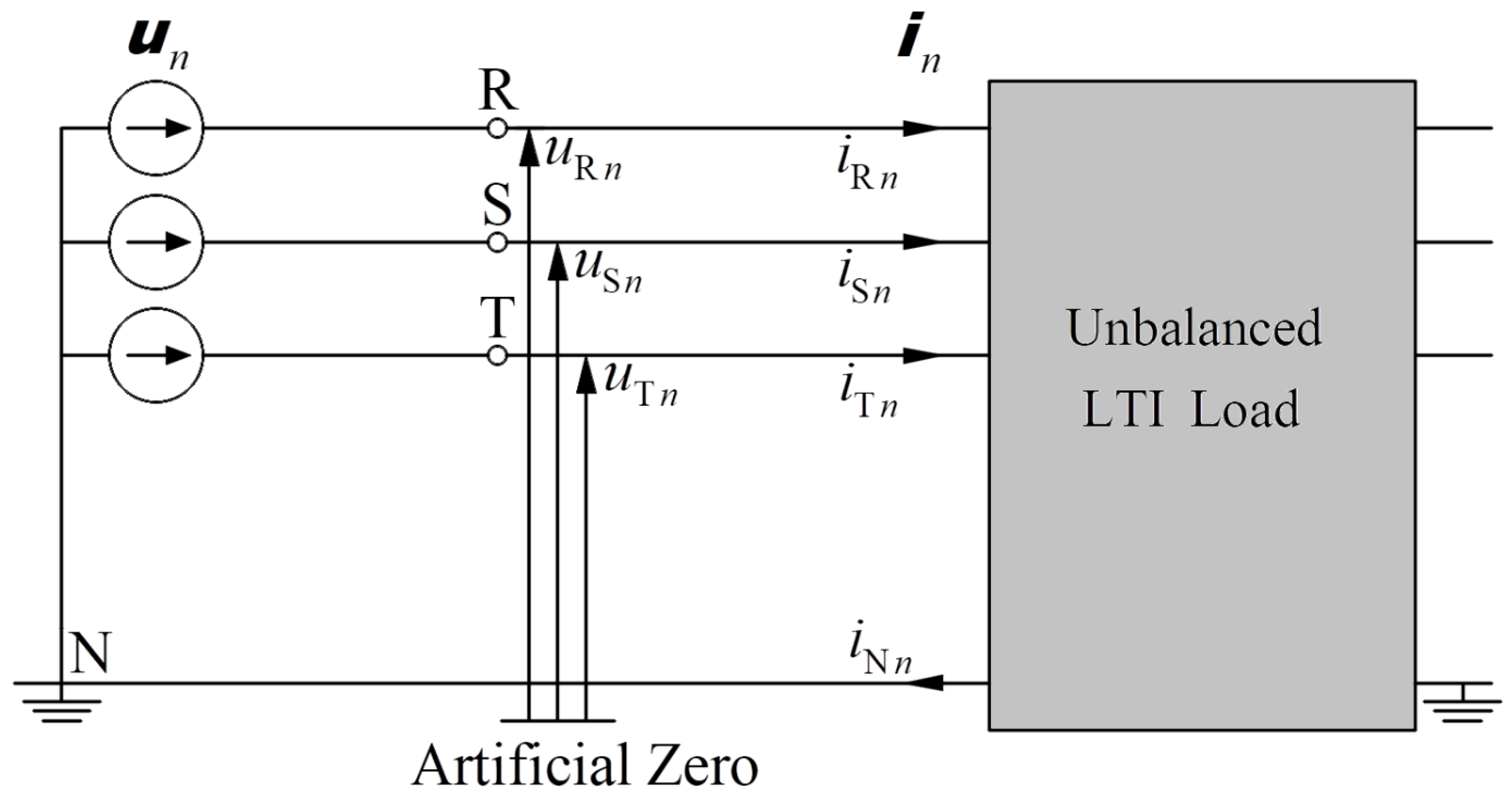
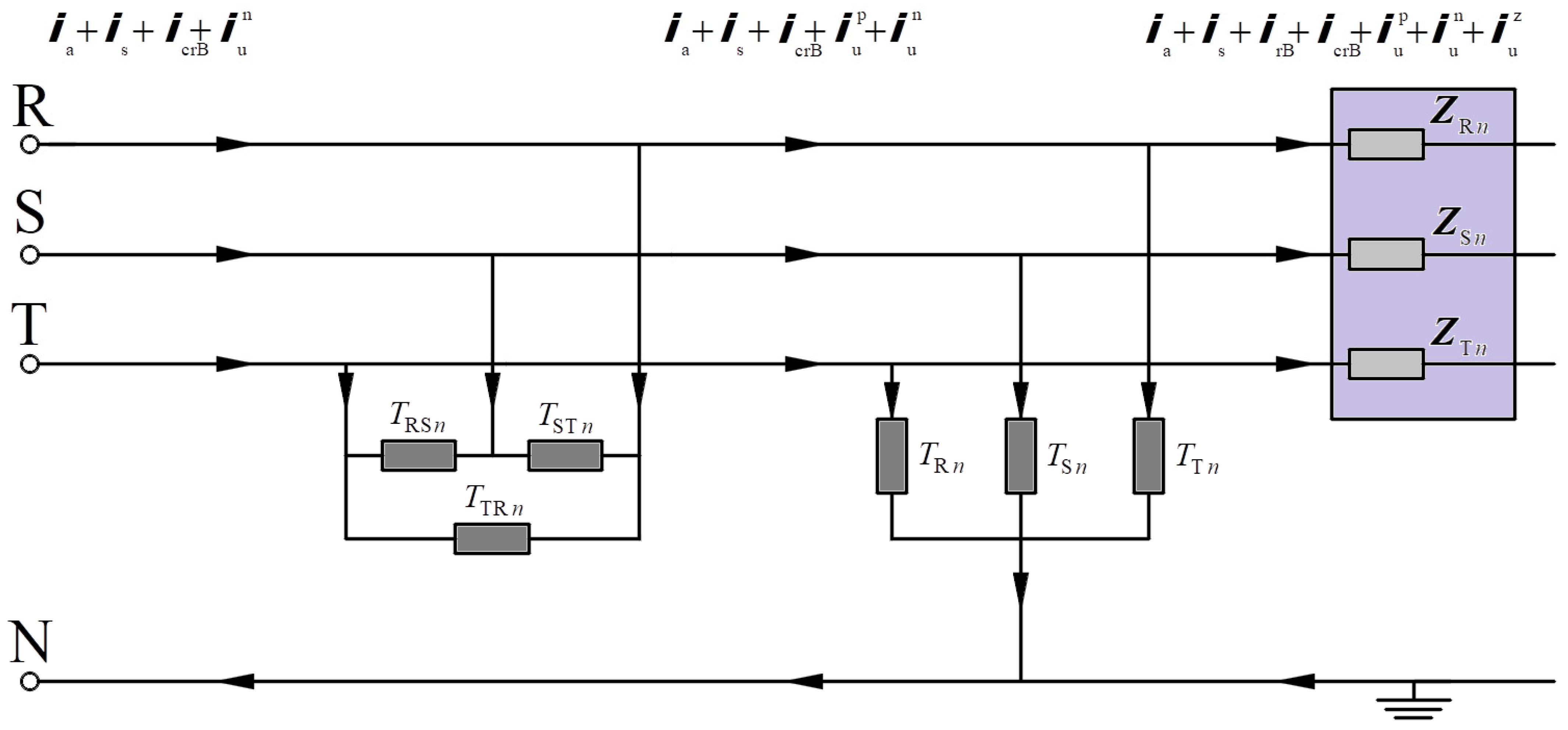
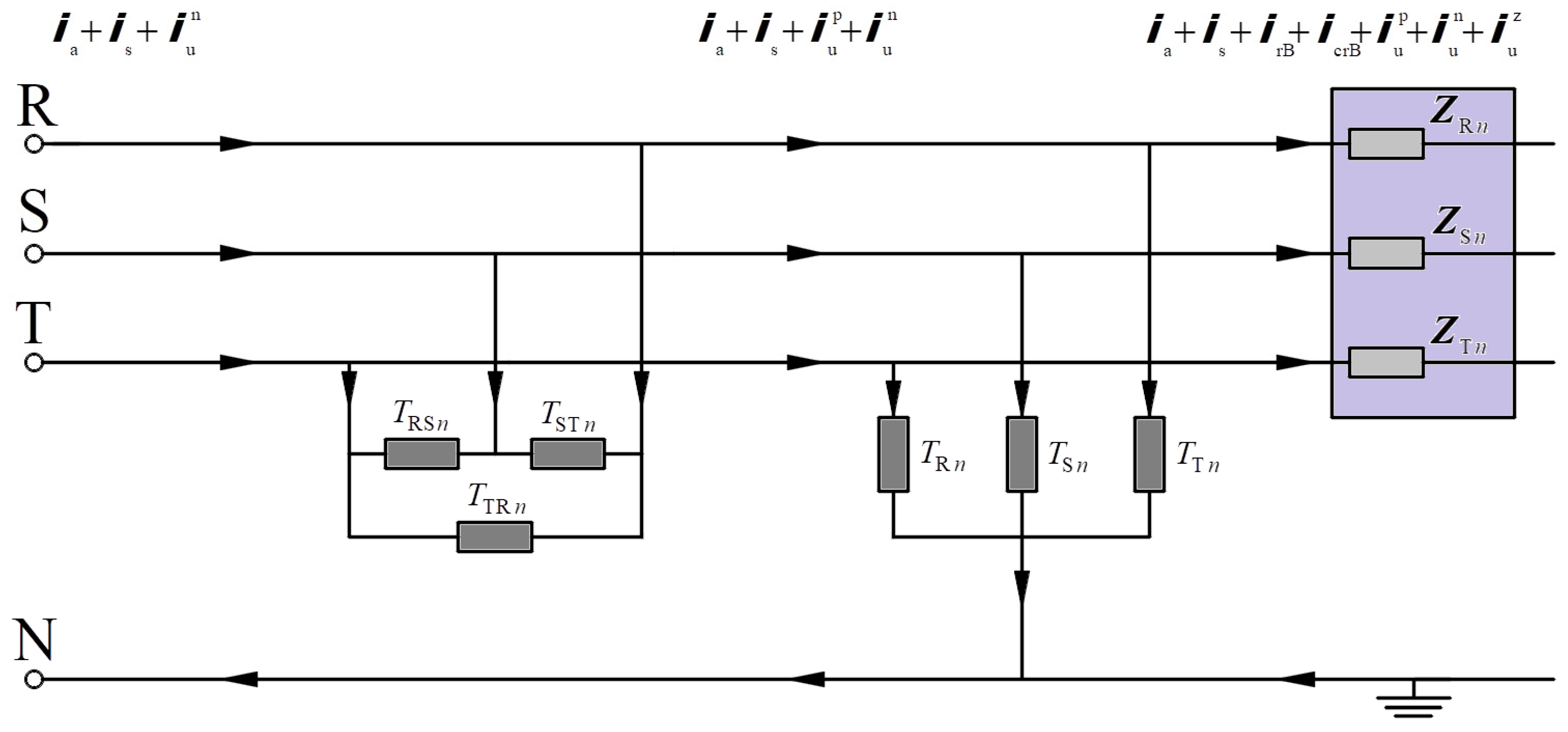
Energies 18 01476 g001
Figure 2. Three-phase four-wire circuit scheme powered by a distorted voltage with an imbalanced linear load.
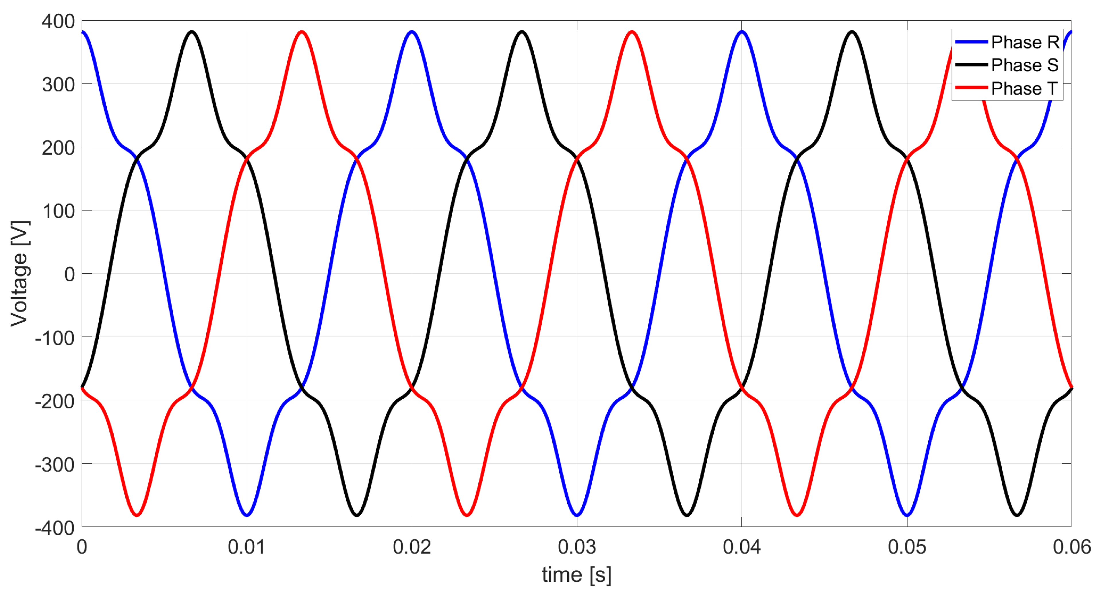
Energies 18 01476 g002
Figure 3. Voltage waveform of a distorted voltage at the connection points of a linear asymmetric load.
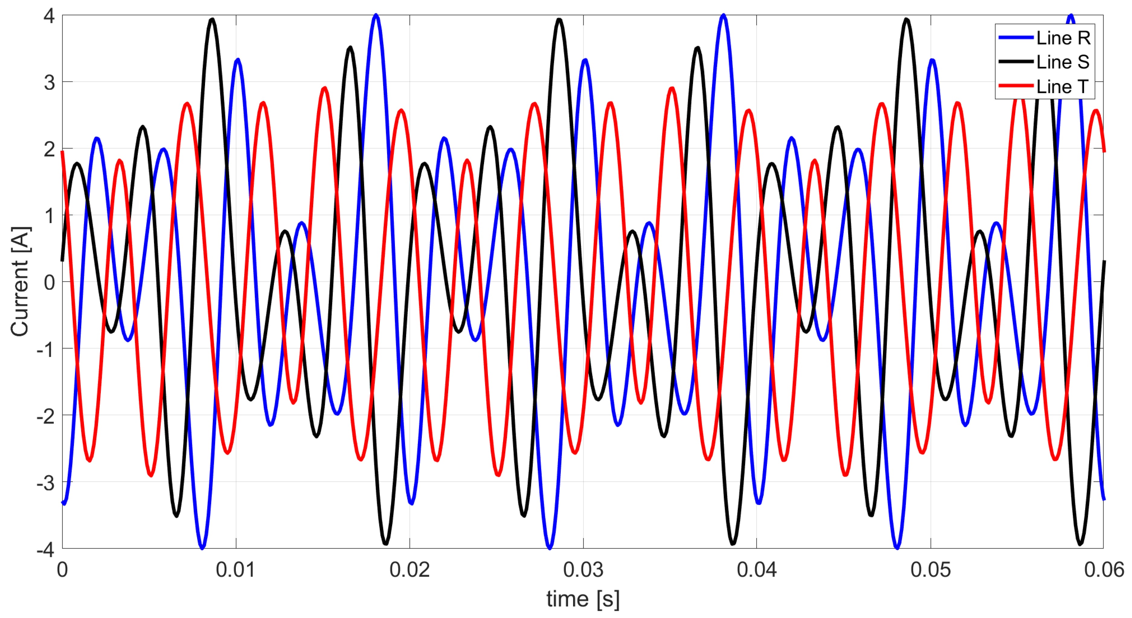
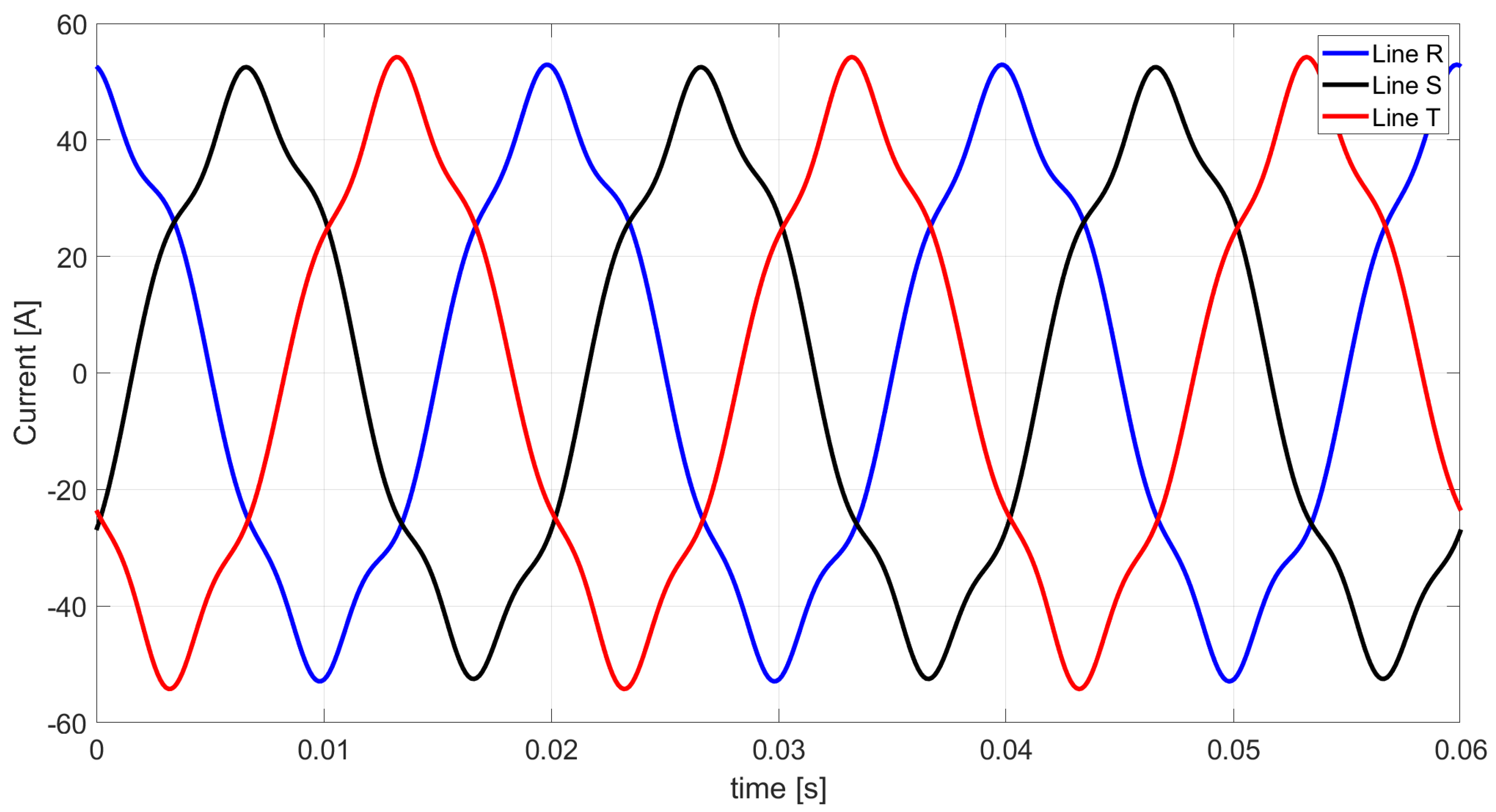
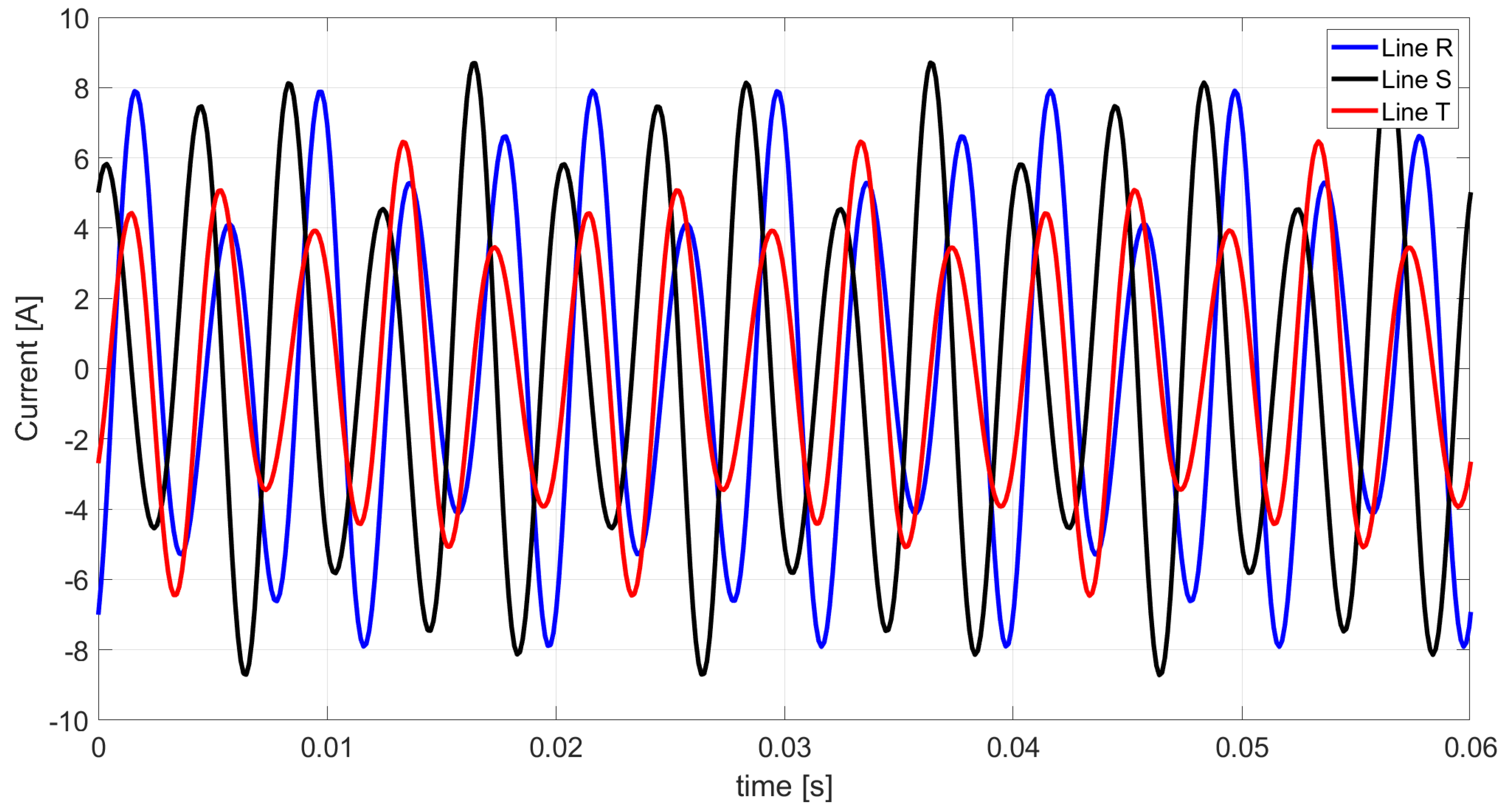
Energies 18 01476 g003
Figure 4. Waveform of line currents obtained from Ohm’s law and Kirchhoff’s law.
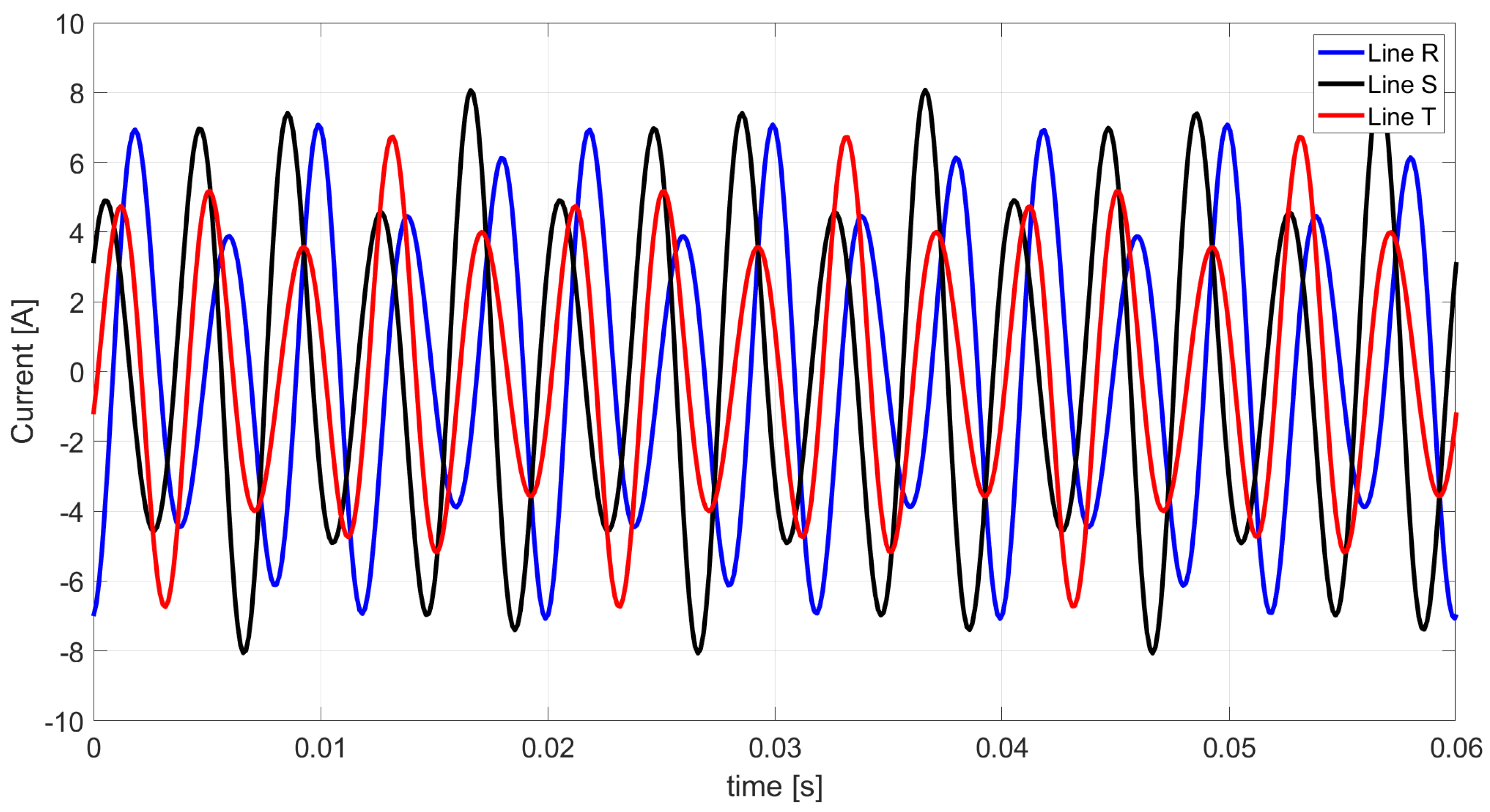
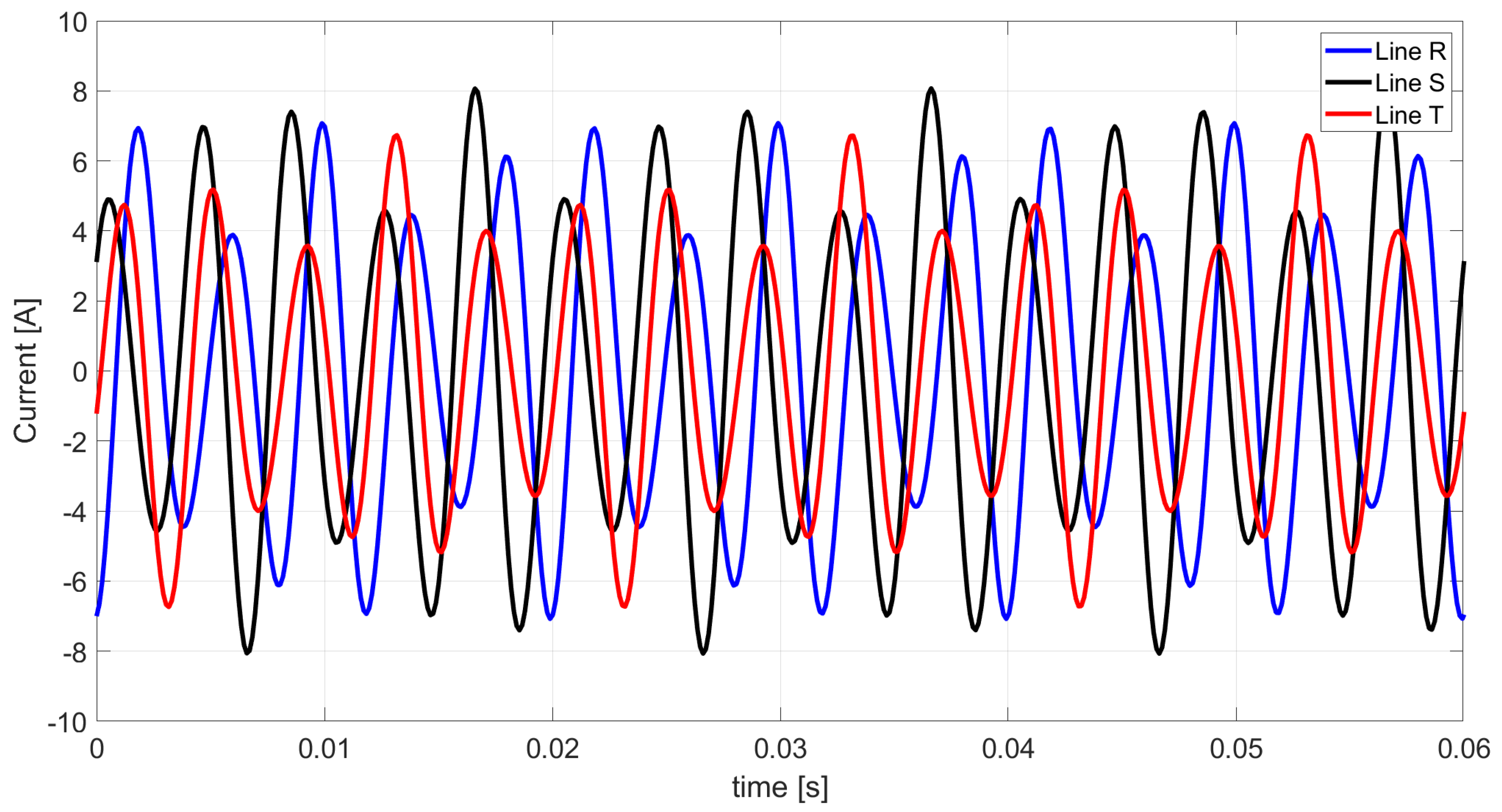
Energies 18 01476 g004
Figure 5. Budeanu distortion current based on the extended Budeanu theory.
Energies 18 01476 g005
Figure 6. View of the primary circuit with the connected compensator responsible for the perfect compensation of the Budeanu complemented reactive current and the unbalanced current.
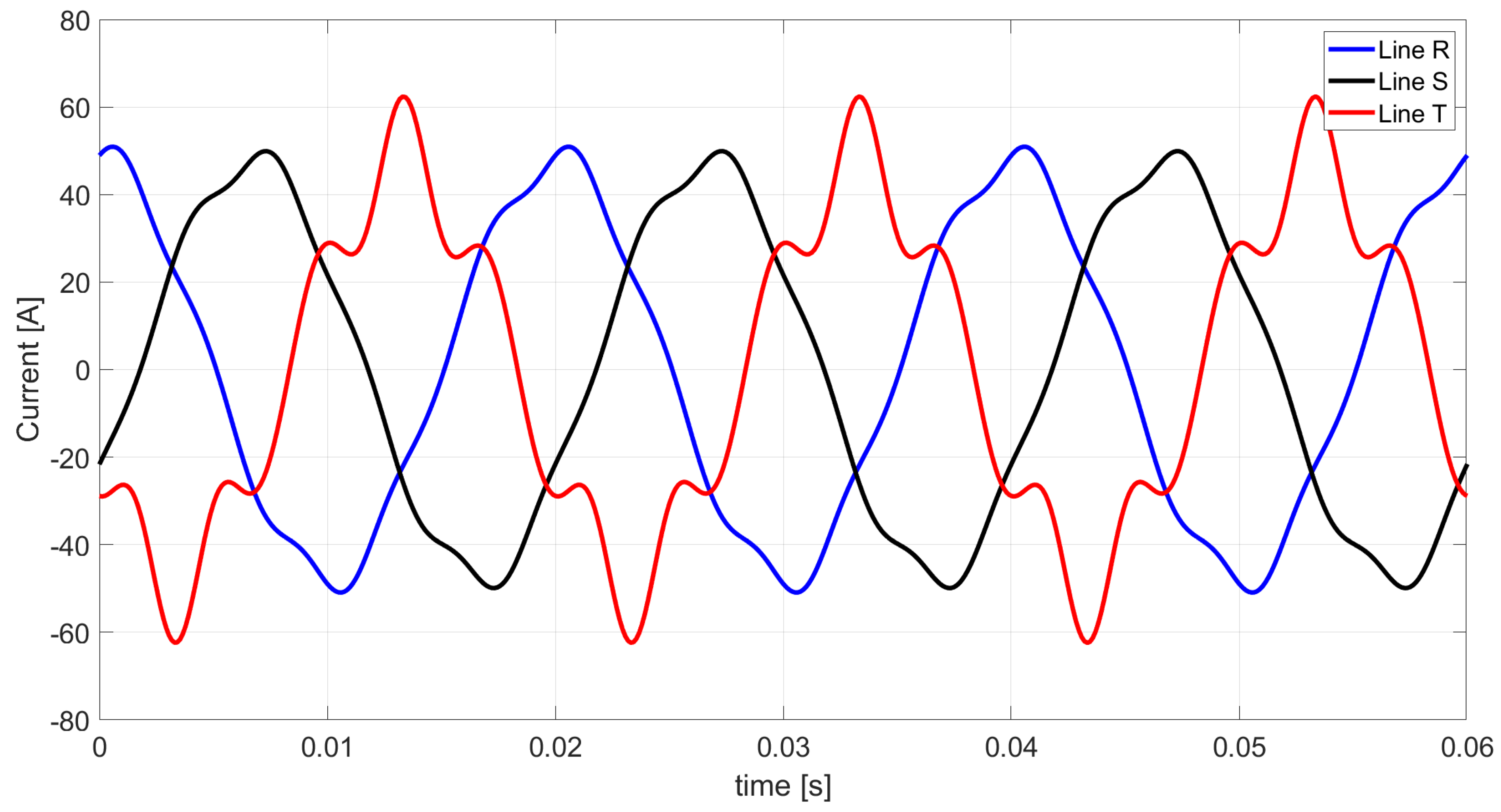
Energies 18 01476 g006
Figure 7. Waveform of the obtained line currents after connecting the compensator of the Budeanu complemented reactive current and the unbalanced current.
Energies 18 01476 g007
Figure 8. Budeanu distortion current waveform according to extended Budeanu theory after compensation of the Budeanu complemented reactive current and the unbalanced current.
Energies 18 01476 g008
Figure 9. View of the primary circuit with the compensator attached, which is responsible for minimizing the Budeanu complemented reactive current and the unbalanced current.
Energies 18 01476 g009
Figure 10. Waveform of the obtained line currents after installing a compensator to minimize the Budeanu complemented reactive current and the unbalanced current.
Energies 18 01476 g010
Figure 11. Budeanu distortion current waveform according to the extended Budeanu theory after minimizing the Budeanu complemented reactive current and the unbalanced current.
Energies 18 01476 g011
Figure 12. View of the receiver with the attached compensator responsible for perfect compensation of the Budeanu reactive current and the unbalanced current.
Energies 18 01476 g012
Figure 13. Waveform of line currents obtained after connecting an ideal Budeanu reactive current and the unbalanced current compensator.
Energies 18 01476 g013
Figure 14. Budeanu distortion current waveform according to the extended Budeanu theory after optimal compensation of the Budeanu reactive current and the unbalanced current.
Energies 18 01476 g014
Figure 15. View of the primary system with the connected compensator responsible for minimizing compensation of the Budeanu reactive current and the unbalanced current.
Energies 18 01476 g015
Figure 16. Waveform of obtained line currents after including a compensator to minimize the Budeanu reactive current and the unbalanced current.
Energies 18 01476 g016
Figure 17. Budeanu distortion current waveform according to the extended Budeanu theory after minimizing the Budeanu reactive current and the unbalanced current.
Energies 18 01476 g017
Figure 18. View of the primary circuit with the attached compensator responsible for perfect compensation of the Budeanu reactive currents and the unbalanced current.
Energies 18 01476 g018
Figure 19. Waveform of the obtained line currents after including an ideal compensator of the Budeanu reactive currents and the unbalanced current.
Energies 18 01476 g019
Figure 20. Budeanu distortion current waveform according to the extended Budeanu theory after ideal compensation of the Budeanu reactive currents and the unbalanced current.
Energies 18 01476 g020
Figure 21. View of the primary system with the connected compensator responsible for minimizing the Budeanu reactive currents and the unbalanced current.
Energies 18 01476 g021
Figure 22. Waveform of the obtained line currents after including a compensator to minimize the Budeanu reactive currents and the unbalanced current.
Energies 18 01476 g022
Figure 23. Budeanu distortion current waveform according to the extended Budeanu theory after minimizing the Budeanu reactive currents and the unbalanced current.
Energies 18 01476 g023
Table 1. Summary of the currents and component powers based on the extended Budeanu theory.
ComponentsQuantityTime WaveformThree-Phase RMS Value
ActiveCurrent i a = G e u = 2 Re n N G e U n e j n ω 1 t i a = G e u = P u
Power- P = u i a
ScatteredCurrent i s = 2 Re n N ( G n G e ) U n e j n ω 1 t i s = n N [ ( G n G e ) 2 u n 2 ]
Power- D s = u i s
Budeanu reactiveCurrent i rB = 2 Re n N j B eB U n e j n ω 1 t i rB = | B eB | u = | Q B | u
Power- Q B = u i rB
Budeanu complemented reactiveCurrent i crB = 2 Re n N [ j ( B n B eB ) ] U n e j n ω 1 t i crB = n N [ ( ( B n B eB ) u n ) 2 ]
Power- Q crB = u i crB
Positive-sequence unbalancedCurrent i u p = 2 Re n N I u n p e j n ω 1 t = 2 Re n N Y u n p 1 p U R n e j n ω 1 t i u p = 3 n N Y u n p U R n
Power- D u p = u i u p
Negative-sequence unbalancedCurrent i u n = 2 Re n N I u n n e j n ω 1 t = 2 Re n N Y u n n 1 n U R n e j n ω 1 t i u n = 3 n N Y u n n U R n
Power- D u n = u i u n
Zero-sequence unbalancedCurrent i u z = 2 Re n N I u n z e j n ω 1 t = 2 Re n N Y u n z 1 z U R n e j n ω 1 t i u z = 3 n N Y u n z U R n
Power- D u z = u i u z
Table 2. Summary of resistance, capacitive reactance, and inductive reactance values for the fundamental harmonics.
Parameter in Ω R-LineS-LineT-Line
Resistance444
Inductive reactance3.1426.283-
Capacitive reactance--1.592
Table 3. Summary of three-phase active power and reactive power values of specific harmonics and the overall three-phase active power and reactive power of the entire system.
Harmonic OrderActive Power P in [W]Reactive Power QB in [VAr]
n = 123,4117872.5
n = 37.42.7
n = 5240.964.2
n = 76.51.3
SUM23,665.87940.7
Table 4. Summary of three-phase RMS values of component currents for individual harmonics described in the extended Budeanu theory.
Harmonic
Order
i a i s i rB i crB i u p i u n i u z
n = 158.3580.40919.5810.180039.27021.599
n = 31.2690.4180.4260.1140.8220.5870
n = 57.6122.9762.5541.3183.83204.745
n = 71.2690.5200.4260.27400.7740.663
RMS58.8803.07719.7561.3633.92039.28222.124
Table 5. Components of the distortion current described in extended Budeanu theory.
Harmonic
Order
i s i crB i u p i u n i u z i dB
n = 10.4090.180039.27021.599
n = 30.4180.1140.8220.5870
n = 52.9761.3183.83204.745
n = 70.5200.27400.7740.663
RMS3.0771.3633.92039.28222.12445.379
Table 6. Summary of capacitance and inductance values required to compensate for the Budeanu complemented reactive current and the unbalanced current for a compensator with a star structure.
LineHarmonic Order
n = 1n = 3n = 5n = 7
C [µF]L [mH]C [µF]L [mH]C [µF]L [mH]C [µF]L [mH]
R-297.58187.1-96.61--3.08
S316.53--8.98-4.1851.22-
T-36.43-10.88-8.44-7.59
Table 7. Summary of capacitance and inductance values required to compensate for the Budeanu complemented reactive current and the unbalanced current for a delta-structure compensator.
LineHarmonic Order
n = 1n = 3n = 5n = 7
C [µF]L [mH]C [µF]L [mH]C [µF]L [mH]C [µF]L [mH]
RS101.10----147.21.04-
ST-57.54--59.90--4.78
TR74.99----7.0942.21-
Table 8. Summary of three-phase active power and reactive power values of individual harmonics and total three-phase active power and reactive power of the whole system after compensation of the Budeanu complemented reactive current and the unbalanced current.
Harmonic OrderActive Power P in [W]Reactive Power QB in [VAr]
n = 123,4117800.6
n = 37.43.7
n = 5240.9132.7
n = 76.53.7
SUM23,665.87940.7
Table 9. Summary of the three-phase RMS values of the currents’ components for the individual harmonics described in the extended Budeanu theory after compensation of the Budeanu complemented reactive current and the unbalanced current.
Harmonic
Order
i a i s i rB i crB i u p i u n i u z
n = 158.3580.40919.5810000
n = 31.2690.4180.426001.2850
n = 57.6122.9762.5540000
n = 71.2690.5200.4260000
RMS58.8803.07719.756001.2850
Table 10. Components of the distortion current defined in extended Budeanu theory.
Harmonic
Order
i s i crB i u p i u n i u z i dB
n = 10.4090000
n = 30.418001.2850
n = 52.9760000
n = 70.5200000
RMS3.077001.28503.335
Table 11. Summary of capacitance and inductance values necessary to minimize the Budeanu complemented reactive current and the unbalanced current for a compensator with a star structure and delta structure.
ParameterConfiguration
StarDelta
RSTRSSTTR
L [mH]313.4672.7536.34227.7657.91307.07
C [µF]-96.72-30.89-22.92
Table 12. Summary of three-phase active power and reactive power values of individual harmonics and total three-phase active power and reactive power of the whole system after compensation of the Budeanu complemented reactive current and the unbalanced current.
Harmonic OrderActive Power P in [W]Reactive Power QB in [VAr]
n = 123,4117724.5
n = 37.44
n = 5240.9133.8
n = 76.52.7
SUM23,665.87865
Table 13. Summary of the 3-phase RMS values of the currents’ components for the individual harmonics described in the extended Budeanu theory after minimizing the Budeanu complemented reactive current and the unbalanced current.
Harmonic
Order
i a i s i rB i crB i u p i u n i u z
n = 158.3580.40919.3940.00400.0580.089
n = 31.2690.4180.4220.0350.7670.6010
n = 57.6122.9762.5300.0454.25204.586
n = 71.2690.5200.4220.11200.7060.671
RMS58.8803.07719.5680.1264.3210.9304.637
Table 14. Components of the distortion current defined in extended Budeanu theory.
Harmonic
Order
i S i crB i u p i u n i u z i dB
n = 10.4090.00400.0580.089
n = 30.4180.0350.7670.6010
n = 52.9760.0454.25204.586
n = 70.5200.11200.7060.671
RMS3.0770.1264.3210.9304.6377.108
Table 15. Summary of capacitance and inductance values required to compensate for the Budeanu reactive current and the unbalanced current for a compensator with a star structure.
LineHarmonic Order
n = 1n = 3n = 5n = 7
C [µF]L [mH]C [µF]L [mH]C [µF]L [mH]C [µF]L [mH]
R120.97-253.2-144.06--6.79
S471.5--18.97-8.1787.98-
T-82.28-30.08-721.0295.31-
Table 16. Summary of capacitance and inductance values required to compensate for the Budeanu reactive current and the unbalanced current for a delta-structure compensator.
LineHarmonic Order
n = 1n = 3n = 5n = 7
C [µF]L [mH]C [µF]L [mH]C [µF]L [mH]C [µF]L [mH]
RS101.10----147.201.04-
ST-57.54--59.90--4.78
TR74.99----7.0942.21-
Table 17. Summary of three-phase power values of individual harmonics and total three-phase power values of the whole system after ideal compensation of the Budeanu reactive current and the unbalanced current.
Harmonic OrderActive Power P in [W]Reactive Power QB in [VAr]
n = 123,41171.9
n = 37.4−1
n = 5240.9−68.5
n = 76.5−2.4
SUM23,665.80
Table 18. Components of the currents for individual harmonics described in the extended Budeanu theory after ideal compensation of the Budeanu reactive current and the unbalanced current.
Harmonic
Order
i a i s i rB i crB i u p i u n i u z
n = 158.3580.40900.180000
n = 31.2690.41800.11401.2850
n = 57.6122.97601.318000
n = 71.2690.52000.274000
RMS58.8803.07701.36301.2850
Table 19. Summary of the three-phase RMS values of the components of the distortion current defined in extended Budeanu theory.
Harmonic
Order
i s i crB i u p i u n i u z i dB
n = 10.4090.180000
n = 30.4180.11401.2850
n = 52.9761.318000
n = 70.5200.274000
RMS3.0771.36301.28503.602
Table 20. Summary of capacitance and inductance values necessary to minimize the Budeanu reactive current and the unbalanced current for a compensator with a star structure and a delta structure.
ParameterConfiguration
StarDelta
RSTRSSTTR
L [mH]190.3648.8382.33227.7657.91307.07
C [µF]36.95144.09-30.89-22.92
Table 21. Summary of three-phase power values of individual harmonics and total three-phase power values of the whole system after minimizing balancing compensation of the Budeanu reactive current and the unbalanced current.
Harmonic OrderActive Power P in [W]Reactive Power QB in [VAr]
n = 123,41114.5
n = 37.43.8
n = 5240.9130.4
n = 76.52.6
SUM23,665.8151.4
Table 22. Summary of the three-phase RMS values of the currents’ components for each harmonic described in the extended Budeanu theory after minimizing balancing compensation of the Budeanu reactive current and the unbalanced current.
Harmonic
Order
i a i s i rB i crB i u p i u n i u z
n = 158.3580.4090.3730.33700.1440.007
n = 31.2690.4180.0080.4350.7840.6350
n = 57.6122.9760.0492.4624.33204.602
n = 71.2690.5200.0080.29300.7050.680
RMS58.8803.0770.3772.5394.4030.9604.652
Table 23. Components of the distortion current defined in extended Budeanu theory.
Harmonic
Order
i s i crB i u p i u n i u z i dB
n = 10.4090.00400.0580.089
n = 30.4180.0350.7670.6010
n = 52.9760.0454.25204.586
n = 70.5200.11200.7060.671
RMS3.0770.1264.3210.9304.6377.607
Table 24. Summary of capacitance and inductance values required for ideal compensation of the Budeanu reactive currents and the unbalanced current for a compensator with a star structure.
LineHarmonic Order
n = 1n = 3n = 5n = 7
C [µF]L [mH]C [µF]L [mH]C [µF]L [mH]C [µF]L [mH]
R122.41-239.30-127.90--4.61
S472.99--15.37-6.1673.58-
T-83.26-21.92-24.25-42.39
Table 25. Summary of capacitance and inductance values required for perfect compensation of the Budeanu reactive currents and the unbalanced current for a delta-structure compensator.
LineHarmonic Order
n = 1n = 3n = 5n = 7
C [µF]L [mH]C [µF]L [mH]C [µF]L [mH]C [µF]L [mH]
RS101.10----147.201.04-
ST-57.54--59.90--4.78
TR74.99----7.0942.21-
Table 26. Summary of three-phase power values of specific harmonics and total three-phase power values of the whole system after perfect compensation of the Budeanu reactive currents and the unbalanced current.
Harmonic OrderActive Power P in [W]Reactive Power QB in [VAr]
n = 123,4110
n = 37.40
n = 5240.90
n = 76.50
SUM23,665.80
Table 27. Values of the components for individual harmonics described in the extended Budeanu theory after ideal compensation of the Budeanu reactive currents and the unbalanced current.
Harmonic
Order
i a i s i rB i crB i u p i u n i u z
n = 158.3580.40900000
n = 31.2690.4180001.2850
n = 57.6122.97600000
n = 71.2690.52000000
RMS58.8803.0770001.2850
Table 28. Components of the distortion current defined in extended Budeanu theory.
Harmonic
Order
i s i crB i u p i u n i u z i dB
n = 10.4090000
n = 30.418001.2850
n = 52.9760000
n = 70.5200000
RMS3.077001.28503.335
Table 29. Summary of capacitance and inductance values necessary to minimize the Budeanu reactive currents and the unbalanced current for a compensator with a star structure and a delta structure.
ParameterConfiguration
StarDelta
RSTRSSTTR
L [mH]188.1248.6983.11227.7657.91307.07
C [µF]37.39144.53-30.89-22.92
Table 30. Summary of three-phase power values of respective harmonics and total three-phase power values of the whole system after minimization of the Budeanu reactive currents and the unbalanced current.
Harmonic OrderActive Power P in [W]Reactive Power QB in [VAr]
n = 123,411−52.9
n = 37.43.8
n = 5240.9130.5
n = 76.52.6
SUM23,665.884
Table 31. Currents’ components for respective harmonics described in the extended Budeanu theory after minimization of the Budeanu reactive currents and the unbalanced current.
Harmonic
Order
i a i s i rB i crB i u p i u n i u z
n = 158.3580.4090.2070.34000.1380.009
n = 31.2690.4180.0050.4390.7840.6350
n = 57.6122.9760.0272.4844.33304.602
n = 71.2690.5200.0050.29700.7050.680
RMS58.8803.0770.2092.5624.4030.9594.652
Table 32. Components of the distortion current defined in extended Budeanu theory.
Harmonic
Order
i s i crB i u p i u n i u z i dB
n = 10.4090.2070.34000.138
n = 30.4180.0050.4390.7840.635
n = 52.9760.0272.4844.3330
n = 70.5200.0050.29700.705
RMS3.0770.2092.5624.4030.9597.615
Table 33. Summary of the three-phase RMS values for the currents’ components for the primary circuit and the circuits after the balancing minimization and perfect compensation are performed.
ComponentOriginal SystemApproach
IIIIII
IdealMiniIdealMiniIdealMini
i a 58.88058.88058.88058.88058.88058.88058.880
i s 3.0773.0773.0773.0773.0773.0773.077
i rB 19.75619.75619.56800.37700.209
i crB 1.36300.1261.3632.53902.562
i u p 3.92004.32104.40304.403
i u n 39.2821.2850.9301.2850.9601.2850.959
i u z 22.12404.63704.65204.652
i dB 45.3793.3357.1083.6027.6073.3357.615
i 76.91862.19562.45258.99059.37058.97459.371
Table 34. Summary of power factors for all considered approaches with ideal compensation and minimizing balancing compensation.
ComponentOriginal SystemApproach
IIIIII
IdealMiniIdealMiniIdealMini
λ 0.7660.9470.9430.9980.9920.9980.992
Table 35. Summary of generalized costs spent on the parts for the construction of a compensator.
ComponentOriginal SystemCost of Approach [u]
IIIIII
IdealMiniIdealMiniIdealMini
choke-126106116
capacitor-4.51.55.5252
SUM-16.57.515.58168
Disclaimer/Publisher’s Note: The statements, opinions and data contained in all publications are solely those of the individual author(s) and contributor(s) and not of MDPI and/or the editor(s). MDPI and/or the editor(s) disclaim responsibility for any injury to people or property resulting from any ideas, methods, instructions or products referred to in the content.

