1. Introduction
Transformer top-oil temperature plays a critical role in detecting transformer faults, as it serves as a key indicator of the internal thermal conditions of a transformer [
1]. Since transformer oil performs essential functions such as cooling and insulation, monitoring its temperature is crucial for ensuring the safe operation and longevity of the equipment. Elevated oil temperatures are directly linked to the degradation of the insulation system, a primary cause of transformer failures [
2,
3].
Research has shown that high oil temperatures lead to chemical breakdowns in insulation materials, which accelerate failure processes. Studies [
4,
5,
6] indicate that abnormally high oil temperatures are often associated with insulation degradation, which compromises the transformer’s performance and shortens its lifespan. Moreover, by combining oil temperature data with operational load factors, it is possible to more accurately predict transformer failures, as these factors together influence the rate of insulation degradation [
7].
The importance of oil temperature in fault detection is further emphasized by studies [
8,
9], which highlight that temperatures exceeding 100 °C significantly accelerate insulation degradation, increasing the likelihood of transformer failure. Additionally, fluctuations in oil temperature can adversely affect transformer health, with sustained high temperatures leading to the rapid deterioration of both the transformer oil and the solid insulating materials [
10]. Research [
11] has also shown that temperatures above 80 °C notably increase the failure rate of transformers.
In conclusion, transformer oil temperature is a vital parameter for early fault detection, as it provides critical insights into the operational health of the transformer. Monitoring and managing oil temperature effectively can prevent transformer failures and enhance the overall reliability and safety of the power system.
Transformer oil temperature has a direct impact on the operational health and longevity of a transformer.
Table 1 outlines specific temperature ranges and the associated effects, each supported by empirical studies. Within the normal operating temperature (max. ~60 °C), transformers typically exhibit stable performance with minimal aging acceleration. Field measurements indicate that under normal loads, top-oil temperatures often remain below about 60 °C [
12]. At these temperatures, both insulation and oil remain chemically stable, and no significant deterioration takes place during normal operational timespans [
13]. Operation in the moderately high-temperature (~60–90 °C) range indicates increased loads or other external stress factors [
12,
14]. Research shows that sustained running within 60–90 °C accelerates oil oxidation and gradually degrades the paper insulation. Although this does not yet occur at a severe rate, operators should monitor it closely, because such modest rises in oil temperature can foreshadow further thermal stress and more pronounced insulation wear if the load remains high [
12,
14,
15]. At high temperatures close to the design limit (~90–110 °C), the oil temperature accelerates the aging process considerably. Accelerated life tests demonstrate that insulation paper deteriorates much faster in this interval [
15,
16]. In particular, some studies note that operating near 110 °C can reduce the expected lifespan of the insulation significantly, sometimes by half compared to normal running temperatures. This zone is often considered the upper boundary for routine operation; each degree above about 100 °C can lead to a notable increase in the aging rate [
17]. Extreme overheating conditions (>~120 °C) can cause rapid and severe damage to oil–paper systems [
18]. Laboratory data suggest that when the hotspot surpasses 120 °C or 130 °C, just a few hours of operation can equate to days of normal aging at 90–100 °C [
16,
18]. The risks in these extreme conditions include rapid insulation breakdown, abrupt gas formation within the oil, and a heightened likelihood of catastrophic failures such as transformer fires. Consequently, it is critical to avoid sustained operation above ~120 °C.
As smart grid technologies advance, the integration of oil temperature monitoring with sophisticated diagnostic systems has garnered increasing attention. By combining oil temperature data at the transformer’s rated load with the temperature rise calculation model outlined in IEEE Std C57.91-2011 [
19], it becomes possible to predict the hotspot temperature rise curve of the transformer under various load conditions [
20]. While traditional forecasting techniques like ARIMA and Support Vector Machines (SVMs) excel at capturing linear trends, they often struggle with more complex fluctuations, such as changes in ambient temperature and load variations [
21,
22]. To address these challenges, an enhanced version of the SVM has been developed, utilizing Particle Swarm Optimization (PSO) to improve accuracy [
23].
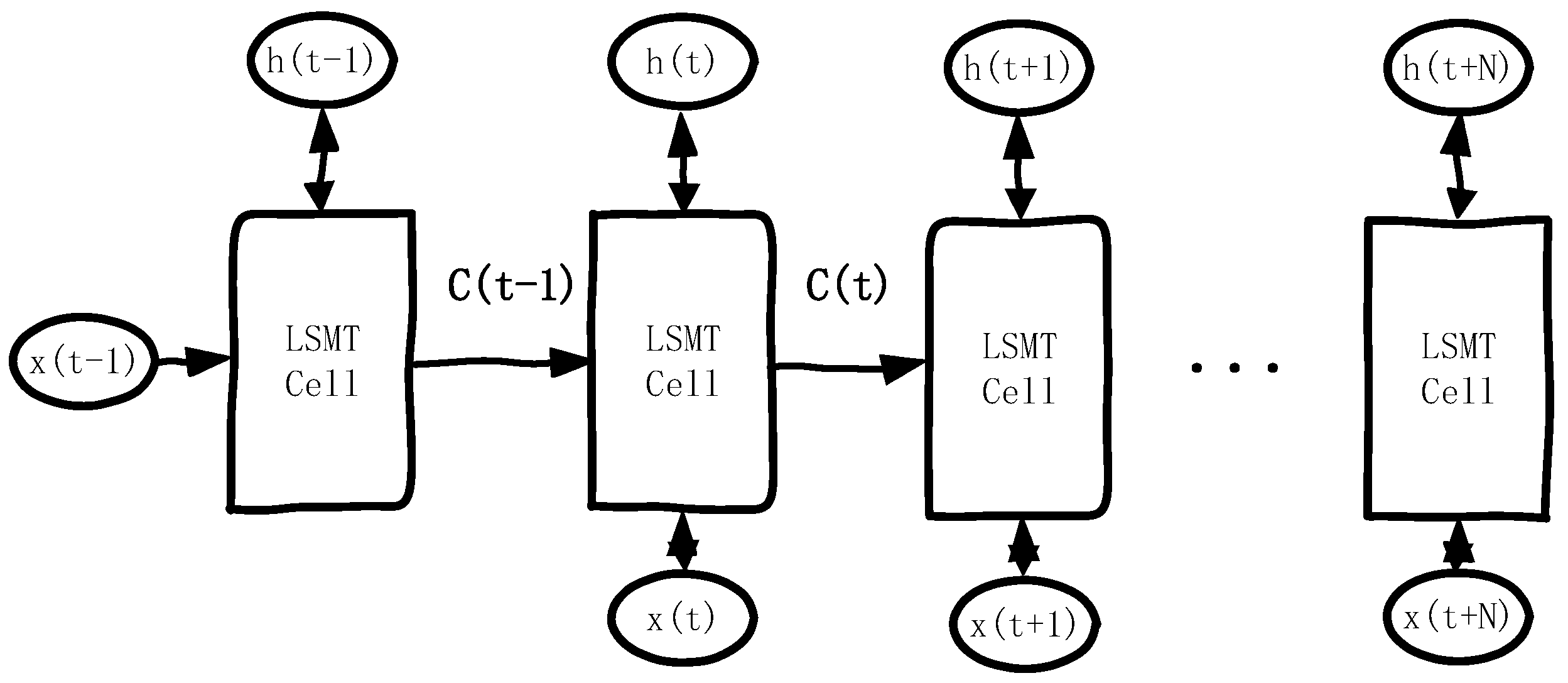
On the other hand, deep learning methods, particularly Long Short-Term Memory (LSTM) networks, have shown great promise in managing nonlinear time series data. However, they typically fail to simultaneously capture both linear and nonlinear features, limiting their overall performance [
24]. To mitigate this, hybrid models have been proposed to predict dissolved gas concentrations in transformer top oil, which aids in fault detection [
16,
25,
26].
In machine learning, Extreme Gradient Boosting (XGBoost) algorithms are widely favored for their efficiency and flexibility, with excellent prediction accuracy, which can quickly and accurately solve various problems in data science [
27]. Combined prediction methods improve the accuracy and stability of prediction by combining the advantages of multiple models and overcoming the limitations of a single model, and this effect has been verified by a wide range of scholars [
28].
This paper introduces an advanced ARIMA-LSTM-XGBoost hybrid model for predicting transformer top-oil temperature changes. The predictions from ARIMA, LSTM, and XGBoost are combined using a linear regression model, which effectively weights and integrates the results. This approach, through linear regression stacking, offers a more efficient and accurate prediction method compared to simpler models like stacking or weighted averaging. The proposed model outperforms the standalone LSTM model in terms of both prediction accuracy and error reduction, making it a robust solution for transformer fault detection.
4. Analysis of the Predicted Result of Oil Temperature at the Top of the Transformer
The power transformer dataset (ETDataset) used in this paper is derived from real measurement data collected between July 2016 and July 2018 by Beijing State Grid Fuda Technology Development Company and the related research team. The dataset was organized, pre-processed, and publicly released in a previous work [
39] and contains real-time oil temperature (OT) and multiple load information for power transformers. During the actual deployment, the team monitored transformer loads from substations in different regions over a long period of time, resulting in a time series covering a two-year time span. For the convenience of academic research, the dataset is subdivided into ETT-small, ETT-large, and ETT-full versions, where ETT-small contains core load and oil temperature monitoring data from multiple (e.g., 2) substations, while ETT-large and ETT-full are more enriched in terms of the number of substations and characterization dimensions, but at the same time, they are also larger.
All visualizations in this paper (e.g., graphs of oil temperature trends, load comparison over time, training sample distribution, etc.) are based on the ETT-small dataset (two years long, with recording intervals of either minutes or hours).
The raw dataset is stored as a csv and each record contains a date and time stamp and the following seven characteristics:
HUFL (High UseFul Load): Effective load data under high-load conditions. They indicate the actual effective use of electricity in high-load scenarios, which is an important reference for evaluating the transformer load status during peak hours.
HULL (High UseLess Load): Invalid load data under high-load conditions. As opposed to HUFL, HULL reflects the wasteful or reactive load during the same high-load period, which is equally important for power dispatch and energy saving and emission reduction analysis.
MUFL (Middle UseFul Load): effective load data under medium-load conditions, used to identify demand during periods of smoother daily electricity use.
MULL (Middle UseLess Load): ineffective load data in medium-load conditions to assist in evaluating load efficiency during off-peak periods.
LUFL (Low UseFul Load): Effective load data under low-load conditions. These reflect the characteristics of the actual active load changes during low-load hours such as late at night.
LULL (Low UseLess Load): Invalid load data under low-load conditions. They are useful for adjusting the operation of power grid equipment during low-load hours and improving the utilization rate.
OT (Oil Temperature): Target variable. As an important index to measure the health condition and load pressure of a power transformer, oil temperature has strong physical meaning, which can effectively reflect the operating condition of the transformer and is very crucial to predict its ultimate load capacity.
In this study, we considered OT as the primary forecasting target and introduced the six load characteristics, “HUFL, HULL, MUFL, MULL, LUFL, and LULL”, and temporal information into the forecasting model to construct a more comprehensive input feature space. This captured both the short-term peak-to-valley fluctuations in electricity consumption and the potential correlation between oil temperature and various loads.
We selected 5000 sets of the above measurements as test data, which are shown and offset in
Figure 4, where OT is the original top-oil temperature data, and LULL, LUFL, MULL, MUFL, HULL, and HUFL are the different characterization data.
In this study, for the transformer oil temperature prediction task, the ARIMA-LSTM model, the XGBoost algorithm, and a hybrid model combining ARIMA-LSTM and XGBoost were used for prediction, respectively. In order to evaluate the prediction effectiveness of each model, four common error metrics were used in this paper: the mean square error (MSE), root mean square error (RMSE), mean absolute error (MAE), and mean absolute percentage error (MAPE). These error metrics helped us quantify the difference between predicted and actual values and compare model performance.
The mean square error (MSE) is one of the most commonly used metrics for evaluating regression problems, which measures the error of a model by calculating the square of the difference between the predicted and actual values and averaging it. The formula is shown in Equation (10):
where
n is the total number of samples;
is the actual value of the ith sample; and
is the predicted value of the ith sample. The smaller the calculated MSE is, the closer the predicted value is to the actual value and the better the model works.
The RMSE is the square root of the MSE, which has the same magnitude as the data unit and is easy to interpret in practical applications. A larger RMSE indicates that the model has a larger error in prediction. The formula is shown in Equation (11):
The MAE is the average of the absolute errors between the predicted and actual values. Unlike the MSE, the MAE is less sensitive to outliers and therefore gives a “fairer” assessment of the error. The formula is shown in Equation (12):
The MAPE, on the other hand, is the average of the absolute value of the prediction error relative to the percentage of the actual value, which is used to assess the proportion of error of the predicted value relative to the actual value and is suitable for analyzing the percentage of error. The calculation method is shown in Equation (13).
The meaning of the variables in the equation is the same as in the above equation: n is the total number of samples; is the actual value of the ith sample; and is the predicted value of the ith sample. The MAPE expresses the magnitude of the error as a percentage, which is applicable to the scenario where the actual value is non-zero, and handles the absolute value of the error, ignoring the positive and negative directions.
In this paper, the auto_arima function of the pmdarima library was used to automatically select the parameters (p, d, q) of the ARIMA model. The function scored and compared the possible parameter combinations by stepwise searching (stepwise = True) and information criteria (e.g., AIC, BIC, etc.) and finally selected the optimal set of lag and difference orders (minimizing the value of the information criteria) automatically. During the experiments, we also kept the trace = True option to see intermediate results of the search process, so as to ensure that the chosen order and number of differences were optimal in terms of the information criterion and that the model fit was good. The final output was the best model: ARIMA (1,1,2).
For the selection of the LSTM model structure and hyperparameters, we used a two-layer LSTM: the first layer contained 100 neurons (units = 100) and the second layer contained 50 neurons (units = 50). For preliminary experiments, we examined single-layer, two-layer, and more-layer (e.g., three- or four-layer) network structures, as well as different numbers of neurons (e.g., 64, 128, etc.). After comparing the training speed, model accuracy, and risk of overfitting, we finally chose this structure to avoid excessive computational overhead while providing better accuracy. The input window size was set to 10, which means that the data of the first 10 time points were used to predict the next time point. This setting was mainly based on the preliminary analysis of the autocorrelation characteristics of the sequence (e.g., period, season, etc.), and in the experiments, we tested the effect of different window lengths, such as 5, 10, 15, 20, etc., and found that time_step = 10 could better balance the prediction accuracy and the efficiency of network training. Meanwhile, Dropout (0.2) was added after each layer of LSTM to suppress overfitting, and the value of 0.2 was chosen after trying several combinations of 0.1, 0.2, 0.3, etc., on the validation set. In addition, the model was trained for a maximum of 300 epochs, but EarlyStopping (patience = 20) was enabled to stop training early and return to the optimal weights when the loss on the validation set did not decrease significantly within 20 epochs. This mechanism effectively prevented the model from overfitting in a later stage and reduced ineffective iterations. LSTM training was performed using the Adam optimizer (optimizer = ‘adam’) with a default learning rate (approximately 0.001). We also tried other optimizers such as SGD and RMSProp and different learning rate settings, but from the performance of the validation set, Adam’s default parameters provided a good balance between convergence speed and stability.
For the part with XGBoost, we performed preliminary tuning, such as setting n_estimators = 100, learning_rate = 0.1, max_depth = 6, etc. These parameters were mainly filtered by grid searching or multiple experimental comparisons (e.g., from 50 to 200 for n_estimators, 0.01 to 0.2 for learning_rate, 3 to 8 for max_depth, etc.). Of course, more refined hyper-parameter optimization methods (e.g., Bayesian optimization, stochastic search, etc.) can be used to improve the model performance in practical applications or more complex datasets.
Finally, we used linear regression as a meta-model to linearly combine the predictions of the previous models (ARIMA + LSTM and XGBoost). The hyperparameters of linear regression were relatively simple, it was mainly used for the process of training the weights, and there were no additional layers or neurons to set. If there was subsequently higher demand for the stacking method, we could consider replacing the meta-model with a more flexible regression algorithm (e.g., XGBoost, MLP, etc.) and further tuning its parameters.
To ensure repeatability and comparability, this paper completed all model training and prediction experiments in a local environment with the following hardware and software configurations:
The hardware configuration was as follows. Processor: Intel (R) Core (TM) i5-14600K @ 3.50 GHz. Memory: 32 GB RAM. OS: Windows 10 Professional Workstation Edition (64-bit, version 22H2). GPU: Integrated Graphics Intel (R) UHD Graphics 770 (training and prediction were mainly performed on the CPU in this study). Python version 3.9.18 (Anaconda distribution). The main third-party libraries used the following: numpy = 1.26.4, pandas = 2.2.3, matplotlib = 3.9.2, scikit-learn = 1.6.1, xgboost = 2.1.3, tensorflow = 2.10.0 (accelerated with MKL), pmdarima = 2.0.4, etc.
Other development tools used were the Integrated Development Environment (IDE) PyCharm 2024 and Anaconda version 24.11.3 for managing the Python environment and dependent packages.
With the above configuration, we completed all experiments including data preprocessing, model construction, training, and evaluation in a single CPU environment. Higher memory and modern CPU frequency ensured good computational efficiency. If readers need GPU acceleration, they can also install the CUDA toolkit (NVIDIA Corporation, Santa Clara, CA, USA) on top of this environment and adjust the TensorFlow/PyTorch version accordingly to achieve faster training speed.
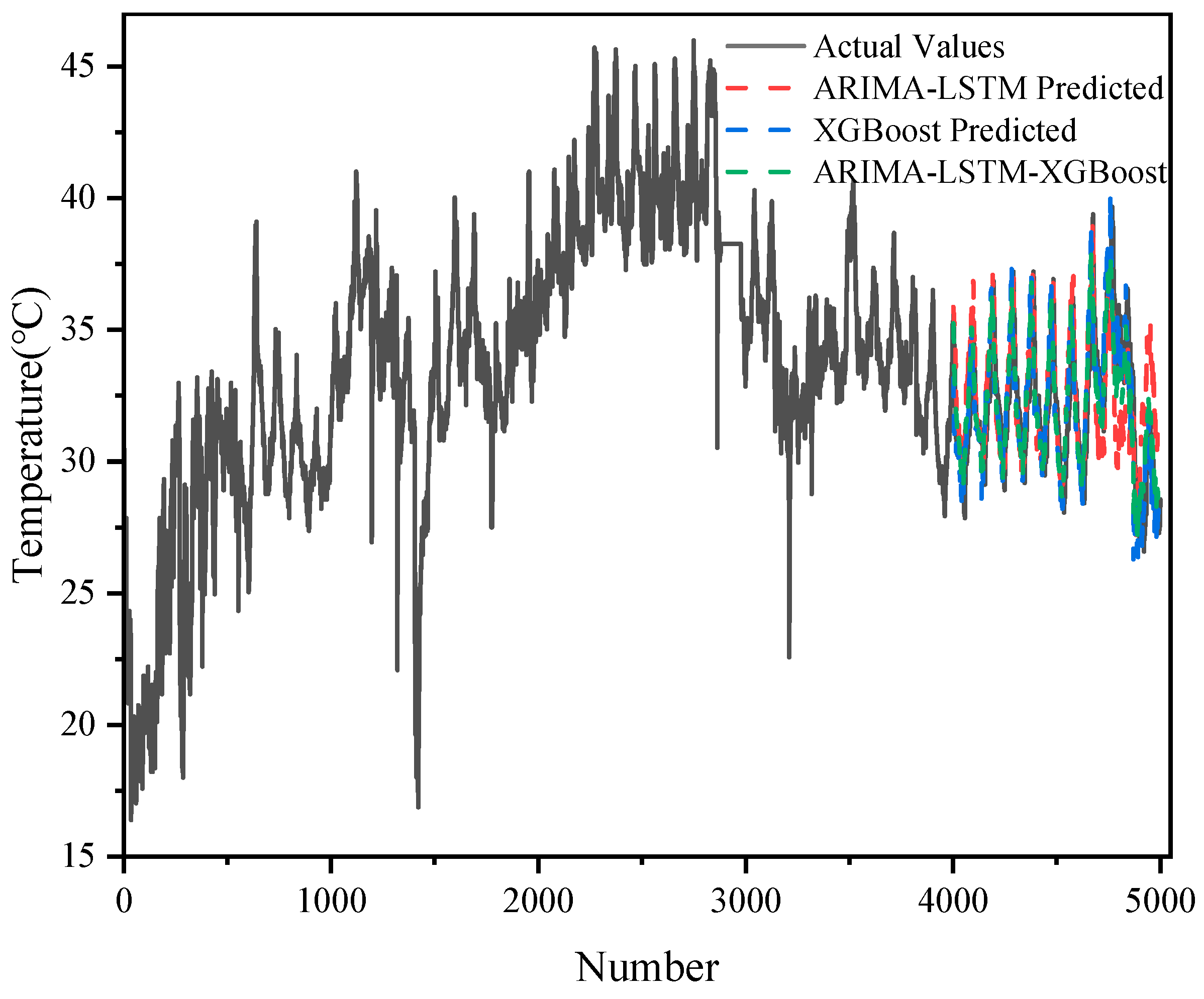
As shown in
Figure 5 and
Figure 6, the results of the prediction of 5000 sets of transformer oil temperature data by the three models (ARIMA-LSTM, XGBoost, and ARIMA-LSTM-XGBoost hybrid model) are demonstrated and compared with the actual oil temperature data (actual values). The graphs show the trend of the actual values with respect to the predicted values of each model.
Although ARIMA-LSTM captured some of the trends in oil temperature changes, there was a certain degree of bias in its prediction results, especially in the region where the data fluctuated a lot, and there was a large difference between the predicted and actual values.
XGBoost was able to capture some nonlinear patterns in the oil temperature data well, but there was a large error in the capture of the overall trend.
The ARIMA-LSTM-XGBoost hybrid model performed best. It combined the linear trend capturing ability of ARIMA, the nonlinear modeling ability of LSTM, and the ability of XGBoost to capture complex patterns and was able to give prediction results closest to the actual values in all samples, with the lowest error, especially in the regions with large data fluctuations.
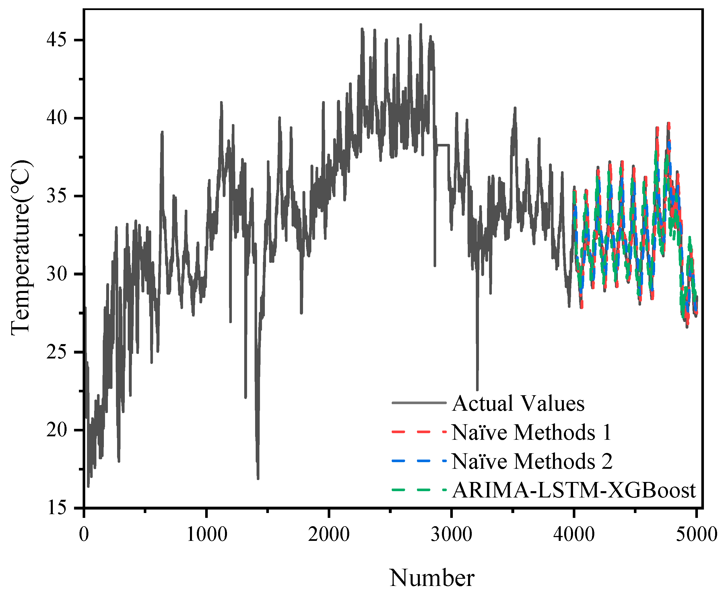
In addition, with the 5000 datasets, we also compared the hybrid model with two naive methods, as shown in
Figure 7 and
Figure 8.
The ARIMA-LSTM model exhibited lower errors (MSE = 1.1268; RMSE = 1.0615; MAE = 0.8883; MAPE = 2.22%), outperforming the XGBoost and naïve methods used alone.
The relatively high error of the XGBoost model (e.g., MSE = 3.2001; RMSE = 1.7889) may be related to its limitations in capturing the temporal and trend nature of the time series. The performance of the two naïve methods was relatively close (MSE around 1.67–1.74, RMSE around 1.29–1.32), and although they were very computationally inexpensive, they fell short when it came to capturing the complex dynamic features of the data.
The ARIMA-LSTM-XGBoost hybrid model further reduced the various error metrics (MSE = 0.9908; RMSE = 0.9954; MAE = 0.7984; MAPE = 1.98%), showing significant performance improvement. This suggests that the hybrid model was able to take full advantage of ARIMA-LSTM’s modeling of temporal features and XGBoost’s ability to capture nonlinear relationships, thus outperforming the single model and simple naïve method in terms of overall prediction accuracy.
The error metrics for the five models are shown in
Table 2.
Based on the comparison of the four error metrics (MSE, RMSE, MAE, and MAPE) mentioned above, the ARIMA-LSTM-XGBoost hybrid model performed the best in all the evaluated metrics, which indicates that the model was able to better capture the changing patterns of the transformer oil temperature data and provide more accurate predictions. The model combined the linear trend capturing ability of the ARIMA model, the nonlinear modeling ability of the LSTM network, and the complex pattern recognition ability of the XGBoost algorithm, resulting in significantly improved prediction accuracy.
In contrast, the XGBoost model performed poorly in all error metrics, and although it was able to capture nonlinear features in the oil temperature data, it was inferior to the ARIMA-LSTM and ARIMA-LSTM-XGBoost combination models in terms of overall prediction accuracy.
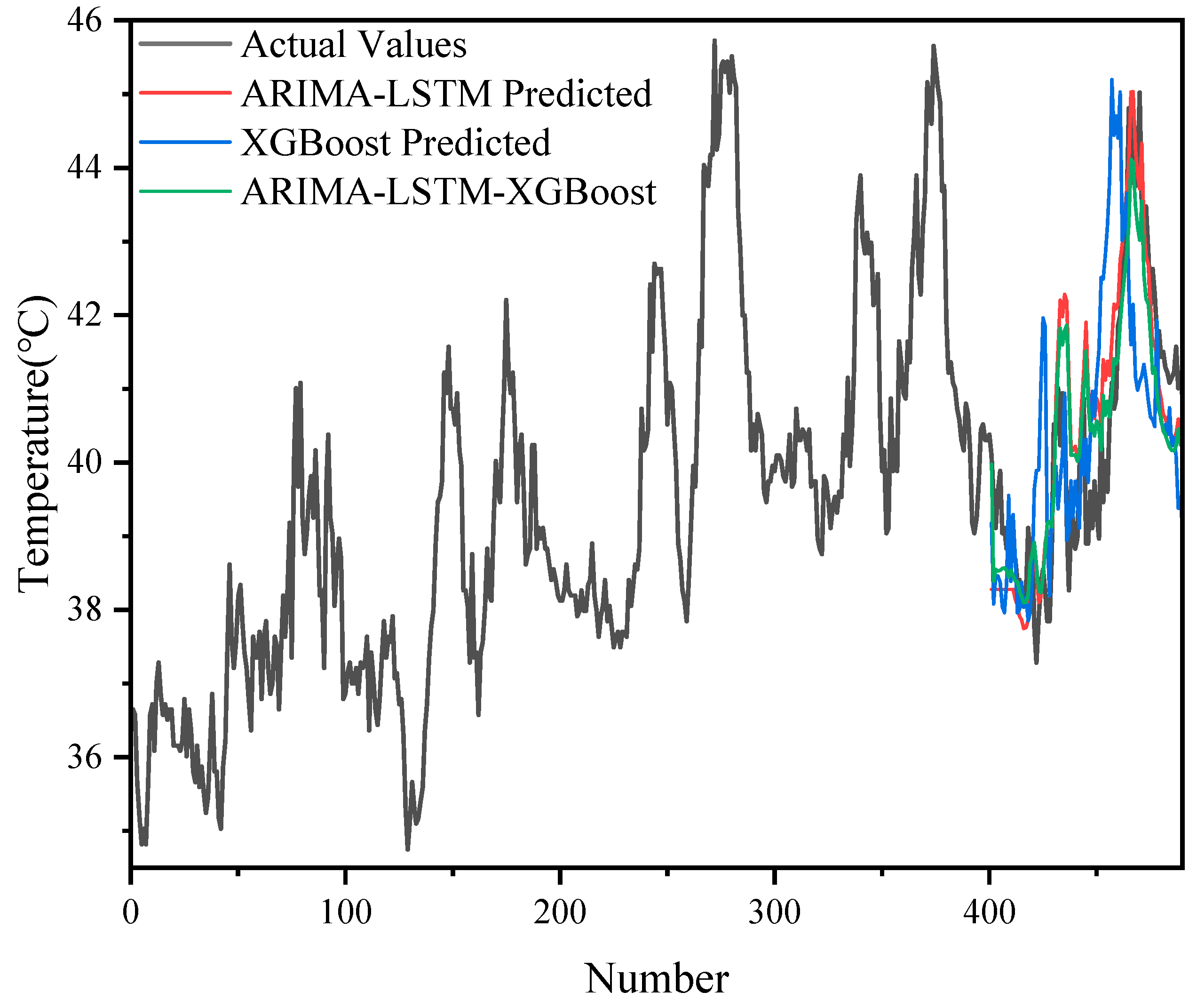
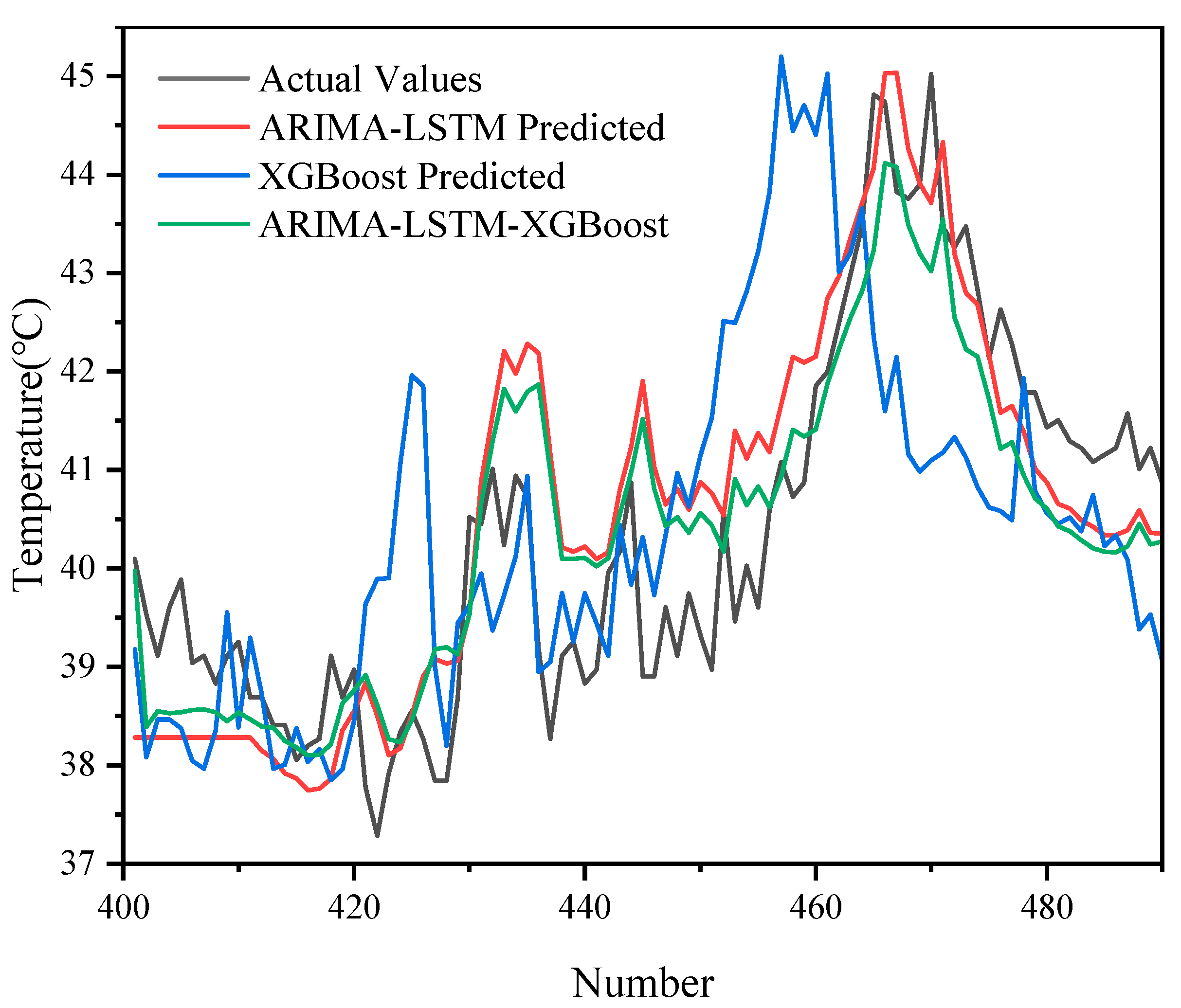
The prediction results of different models (ARIMA-LSTM, XGBoost, ARIMA-LSTM-XGBoost) on 500 sets of data are demonstrated in
Figure 9 and
Figure 10, and it can be seen that the ARIMA-LSTM model captured the overall trend of the oil temperature better, but there was still some prediction bias in some periods, especially in the period of large fluctuations in the model. The prediction error of XGBoost was still more obvious in some periods with large fluctuations, and it could not follow the changes in the actual values accurately. The ARIMA-LSTM-XGBoost hybrid model had the highest prediction accuracy at all time points and could most accurately simulate the fluctuation in oil temperature data.
Similarly, we also compared the naive approaches with the hybrid model in the case of 500 sets of data, and the results are shown in
Figure 11 and
Figure 12.
Overall, the error metrics for each model increased compared to those for the 5000 datasets, reflecting the significant impact of data volume on model training and prediction effectiveness.
Although the performance of the ARIMA-LSTM model decreased significantly with reduced data volume (MSE = 3.6481; RMSE = 1.9100), the hybrid model ARIMA-LSTM-XGBoost was still able to maintain low errors (MSE = 1.9174; RMSE = 1.3847; MAPE = 3.63%), which demonstrates that it was more robust when data were scarce.
Compared with XGBoost (MSE = 2.4710; RMSE = 1.5719) and the naïve methods (MSE about 2.86–2.97), the hybrid model still achieved better prediction results with limited data volume, which further validates its advantages.
Table 3 shows the results of the comparison of the error metrics (MSE, RMSE, MAE, and MAPE) of the five models on 500 sets of data.
Through the above comparison, we can see that although the naïve methods have obvious computational advantages and can provide reasonable predictions in some simple cases, its shortcomings are the following: it is weak in modeling nonlinear and complex dynamic relationships, and it makes it easy to ignore the potential characteristics of the data.
Complex models, especially hybrid models, on the other hand, by integrating the strengths of statistical and machine learning methods, not only improve prediction accuracy but also show better adaptability when facing datasets of different sizes. Although the computational burden of hybrid models is higher than that of naïve methods, the experimental results show that the improvement in prediction accuracy is enough to make up for this disadvantage, especially in scenarios where prediction accuracy is required to be high in practical applications; complex models are more capable of meeting these practical needs.
The XGBoost model outperformed the ARIMA-LSTM, especially in the MSE and RMSE metrics, where it showed lower prediction errors. The ARIMA-LSTM-XGBoost hybrid model performed the best in all the error metrics, especially in the MSE, RMSE, and MAE, where it showed the smallest errors, proving that the hybrid model had an obvious advantage.
The XGBoost model did not perform as well as ARIMA-LSTM in the prediction results on 5000 sets of data. The reason for this phenomenon may be that although the XGBoost model is able to capture complex nonlinear features when dealing with large-scale data, it is weak in recognizing global patterns in data, which leads to a shortfall in capturing the overall trend. ARIMA-LSTM, on the other hand, is able to capture linear trends through the AR and MA processes, which, combined with the nonlinear modeling of LSTM, can better accommodate patterns in large-scale data.
However, the XGBoost model outperformed ARIMA-LSTM in the prediction with 500 sets of data. This may be due to the fact that the 500 sets of data were simpler, and XGBoost was able to deal better with the nonlinear features and fluctuating trends in them, whereas ARIMA-LSTM failed to take full advantage of its strengths. In this case, XGBoost was able to quickly capture the nonlinear changes in the data through the gradient boosting algorithm, thus improving the prediction accuracy.
From the above analysis, it can be seen that the ARIMA-LSTM-XGBoost hybrid model performed well on datasets of different sizes, especially in capturing complex patterns and high-volatility components. By combining the linear trend of ARIMA, the nonlinear modeling capability of LSTM, and the powerful pattern recognition capability of XGBoost, the hybrid model effectively compensated for the shortcomings of a single model and significantly improved the prediction accuracy. The combined model was able to provide the most accurate prediction results for both large-scale data (5000 sets of data) and small-scale data (500 sets of data) prediction tasks, proving its effectiveness and superiority in transformer oil temperature prediction tasks.


