An Adaptive Energy Management Strategy for Off-Road Hybrid Tracked Vehicles

Abstract

Conventional energy management strategies based on reinforcement learning often fail to achieve their intended performance when applied to driving conditions that significantly deviate from their training conditions. Therefore, the conventional reinforcement-learning-based strategy is not suitable for complex off-road conditions. This research suggests an energy management strategy for hybrid tracked vehicles operating in off-road conditions that is based on adaptive reinforcement learning. Power demand is described using a Markov chain model that is updated online in a recursive way. The technique updates the MC model and recalculates the reinforcement learning algorithm using the intrinsic matrix norm (IMN) as a criteria. According to the simulation results, the suggested method can increase the adaptability of energy management based on the reinforcement learning strategy in off-road conditions, as evidenced by the 7.66% reduction in equivalent fuel consumption when compared with the conventional Q-learning based energy management strategy.

1. Introduction

Hybrid tracked vehicles equipped with multiple power sources are characterized by their low fuel consumption and high maneuverability [1]. The power distribution among various power sources in hybrid vehicles is a difficult nonlinear problem with several inputs and variables. According to their methods of solution, rule-based and optimization-based strategies are the two main categories into which the energy management problem of hybrid vehicles can be divided in the current research. Although rule-based solutions are straightforward and quick to execute in engineering, they are unlikely to produce the best control results. They frequently set threshold values based on engineering knowledge to regulate the system [2,3]. In contrast, optimization-based strategies establish objective functions and employ various global or instantaneous optimization algorithms to solve the problem, resulting in superior control schemes [4]. Global optimization strategies, based on prior knowledge of complete driving cycles, can yield globally optimal control decision-making schemes. Commonly used algorithms include the Pontryagin’s Minimum Principle (PMP) [5], convex optimization (CO) [6], and dynamic programming (DP) [7,8], among others. However, driving cycles are often unpredictable in practical applications; hence, global optimization algorithms are usually employed as benchmark methods to evaluate other strategies. Instantaneous optimization strategies, on the other hand, overcome this challenge by making immediate decisions based on past and instantaneous information, resulting in relatively optimized control strategies. Common instantaneous optimization strategies include model predictive control (MPC) [9] and the equivalent consumption minimization strategy (ECMS) [10]. Real-time optimization algorithms are rapid in response and better suited for decision-making in unknown conditions, although they cannot guarantee globally optimal control solutions.

Due to rapid advancements in machine learning, intelligent algorithms have also been applied in the field of energy management in recent years. Among the many intelligent algorithms, reinforcement learning (RL) [11,12,13] and various types of neural networks (NNs) [14,15,16] are common algorithms used in intelligent strategies for energy management. Among these, reinforcement learning has gained increasing application in energy management issues due to its favorable real-time performance and its ability to achieve results that are close to global optimality. For instance, Sun et al. [17] proposed a reinforcement learning strategy with adaptive fuzzy filtering and ECMS to enhance computational efficiency and optimize energy consumption in vehicle power systems. Lian et al. [18] introduced battery performance and optimal braking fuel consumption curves into a deep reinforcement learning algorithm to reduce the control space during energy management, resulting in a more stable, rapid, and easily generalizable control system. Xu et al. [19] investigated the impact of parameter selection and quantity on the effectiveness of energy management strategies based on reinforcement learning. Liu et al. [20] demonstrated the computational time superiority of reinforcement learning algorithms by comparing the performance of two different reinforcement learning algorithms with stochastic dynamic programming algorithms.

The performance of reinforcement-learning-based energy management strategies is highly dependent on training datasets representing limited operational conditions. When there is a significant discrepancy between the actual application conditions and the training datasets, a severe degradation in energy management performance may occur. Consequently, reinforcement learning has found favorable applications in buses, vehicles in closed environments, and rail vehicles. However, due to the complex and variable off-road conditions encountered by tracked vehicles, traditional reinforcement learning methods lack the adaptability to diverse driving conditions, making it difficult to maintain a satisfactory control effect.

Addressing this issue, this paper introduces a new model-based reinforcement learning approach. Initially, a high-order Markov chain model is used to describe the demand power in off-road environments. The model is updated dynamically based on the current vehicle state. When the changes in the Markov chain exceed a predefined threshold, an online update of the reinforcement learning strategy is induced. This enhances the adaptability of the energy management strategy for tracked vehicles, enabling it to achieve favorable results under complex off-road conditions.

The remainder of this paper is structured as follows. Section 2 presents the configuration and modeling methodology for hybrid electric vehicles (HEVs), along with the formulation of the optimal control problem addressed in this study. Section 3 develops an adaptive reinforcement learning-based energy management strategy utilizing a high-order Markov chain model. Section 4 provides a comprehensive validation and evaluation of the proposed control strategy. Finally, Section 5 concludes the paper with a summary of the key findings and contributions.

2. Modeling and Optimal Control Problem

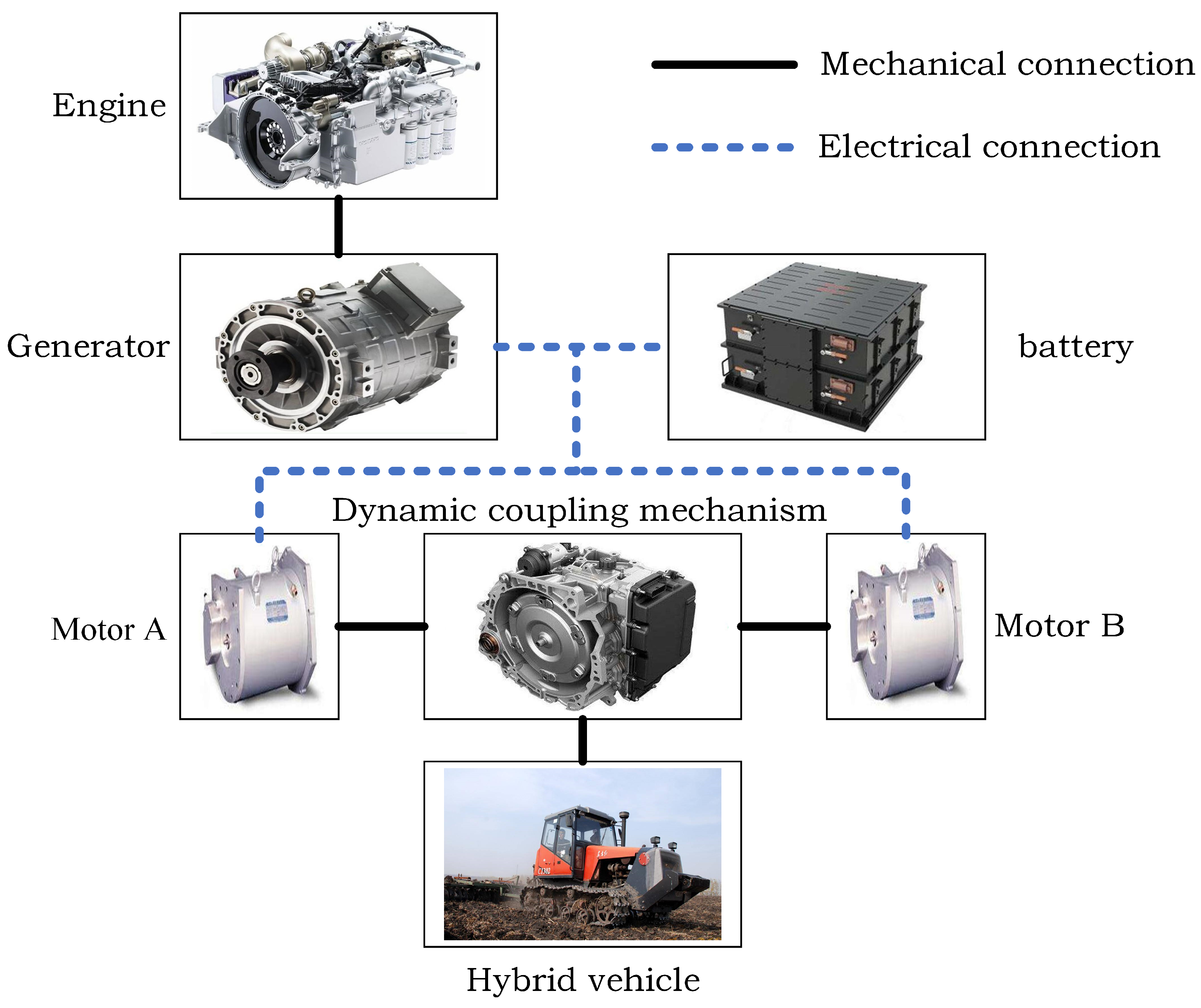
2.1. Hybrid Vehicle Configuration

An engine–generator set (EGS), a power battery, and two driving motors make up the majority of the powertrain system of the series hybrid tracked vehicle that is the subject of this study. According to the system topology shown in Figure 1, these parts are connected to the DC bus. While the driving motors use electricity to move the hybrid tracked vehicle forward, the EGS and the power battery together provide the vehicle with electrical power. The particular parameter settings for the series hybrid tracked vehicle under investigation are shown in

Table 1. Parameters of the HEV.

Name	Value	Unit
Vehicle mass M	25,000	kg
Minimum State of Charge $SO{C}_{min}$	0.3	/
Maximum State of Charge $SO{C}_{max}$	0.9	/
Battery capacity $C_b$	80	Ah
Engine inertia $J_{eg}$	3	$\mathrm{kg}·{\mathrm{m}}^2$
Windward area A	5	${\mathrm{m}}^2$
Air resistance coefficient $C_d$	0.6	/

.

2.2. Modeling the Hybrid Tracked Vehicle

The system model of the vehicle, comprising the engine–generator set model, the power battery model, and the vehicle dynamics model, has been created to solve the power management challenges of series hybrid tracked vehicles.

The engine’s maximum speed in this study is 3800 rpm, while its idle speed is set at 2000 rpm. With a rated torque of 2000 $\mathrm{N}·\mathrm{m}$ within the engine’s operational speed range, the generator can be thought of as a permanent magnet synchronous motor (PMSM). The torque output delay is represented by a first-order inertial element, which ignores transient processes and other small effects during engine operation. The engine’s external characteristic data are used to create the engine’s dynamic model.

$$\begin{array}{c}\hfill \left\{\begin{array}{c}{\dot{T}}_e={\displaystyle \frac{\alpha ·f\left(n_e\right)-T_e}{\tau }}\hfill \\ {\displaystyle \frac{\pi }{30}}·J_{eg}·{\dot{n}}_e=T_e-T_g-{\displaystyle \frac{\pi }{30}}·m_{eg}·n_e\hfill \\ P_g=U_g·I_g={\displaystyle \frac{T_g·n_g·{\eta }_g}{9549}}\hfill \end{array}\right.\end{array}$$

(1)

where $J_{eg}$ is the EGS’s moment of inertia, $n_e$ is the engine speed, and $m_e$ is the engine’s equivalent resistance coefficient. $T_e$ is the engine output torque, $\tau$ is the engine torque output delay time, $\alpha$ is the engine throttle, and $f\left(n_e\right)$ is the function of the external characteristics of the engine torque with regard to the speed. $T_g$ represents the generator’s output torque, ${\eta }_g$ its efficiency, $U_g$ its output voltage, and $I_g$ its output current. Using the battery’s internal resistance model, we can determine:

$$\begin{array}{c}\hfill \left\{\begin{array}{c}{\displaystyle \frac{\mathrm{d}SOC}{\mathrm{d}t}}={\displaystyle \frac{I_b}{C_b}}\hfill \\ U_b=V_{oc}-I_b·r_{int}\hfill \\ P_b=U_b·I_b\hfill \end{array}\right.\end{array}$$

(2)

where $I_b$ represents the current of battery, $r_{int}$ represents the internal resistance, $SOC$ represents the state of charge, $C_b$ represents the battery’s capacity, $U_b$ represents the battery voltage, and $V_{oc}$ represents the battery’s open circuit voltage.

The dynamic model of the vehicle can be written as follows:

$$\begin{array}{c}\hfill P_{dem}=v(Mgfcos\alpha +Mgsin\alpha +{\displaystyle \frac{C_{d}A}{21.25}}{v}^2+\delta M{\displaystyle \frac{\mathrm{d}v}{\mathrm{d}t}})\end{array}$$

(3)

where M is the total mass of the vehicle, g is the gravitational coefficient, f is the ground resistance coefficient, $\alpha$ indicates the road’s inclination angle, $C_d$ is the air resistance coefficient, A is the windward area, v is the vehicle driving speed, and $P_{dem}$ is the power needed for vehicle driving.

2.3. Optimal Control Problem

The speed and torque of the engine are chosen as the control variable $A=[n_e,T_e]$ in the context of energy management, while the post-powertrain’s power demand and the battery’s state of charge (SOC) are chosen as state variables $S=[P_{dem},SOC]$. Energy management aims to minimize excessive engine speed fluctuations, maintain a reasonable battery state of charge, and maximize fuel efficiency. Consequently, the following is the definition of the cost function:

$$\begin{array}{c}\hfill \left\{\begin{array}{c}J={\displaystyle \sum _{k=0}^{N-1}}({\dot{m}}_f\left(k\right)+{\beta }_1{(\Delta SOC\left(k\right))}^2+{\beta }_2{(\Delta n_e\left(k\right))}^2)\hfill \\ \Delta SOC\left(k\right)=SOC\left(k\right)-SO{C}_{pre}\hfill \\ \Delta n_e\left(k\right)=n_e\left(k\right)-n_e(k-1)\hfill \end{array}\right.\end{array}$$

(4)

where the time period is denoted by N, a specific moment in time by k, the fuel consumption rate by ${\dot{m}}_f$, the weight coefficient by ${\beta }_1,{\beta }_2>0$, and the $SO{C}_{pre}$, a predefined constant that keeps the SOC within a tolerable range. Additionally, the variables are subject to the following inequalities when the control strategy is being developed:

$$\begin{array}{c}\hfill \left\{\begin{array}{c}SO{C}_{min}\le SOC\le SO{C}_{max}\hfill \\ T_{g,min}\le T_g\left(k\right)\le T_{g,max}\hfill \\ n_{e,min}\le n_e\left(k\right)\le n_{e,max}\hfill \end{array}\right.\end{array}$$

(5)

3. Adaptive Reinforcement-Learning-Based Energy Management Strategy

3.1. Demand Power Model Based on Online-Updated Markov Chain

3.1.1. Higher-Order Markov Chain

Typical higher-order Markov chains (MCs) become unmanageable for efficient estimation as their processing overhead grows exponentially with the rising order k and number of possible states n. A unique model is provided that mimics the traditional higher-order MC with fewer parameters.The transition probability of the hth-order MC can be expressed as follows when the vehicle’s demand power is selected as the state variable:

$$\begin{array}{c}\hfill \begin{array}{cc}\hfill & P(P_{dem,t}=l_t\mid P_{dem,1}=l_1,\dots ,P_{dem,t-1}=l_{t-1})\hfill \\ \hfill & =q_{l_{t-h},\dots ,l_t}=\sum _{i=1}^h{\lambda }_i{q}_{kj}^i\hfill \\ \hfill & ={\displaystyle \frac{C_{l_{t-h},\dots ,l_t}}{C_{l_{t-h},\dots ,l_{t-1}}}}\hfill \\ \hfill & C_{l_{t-h},\dots ,l_{t-1}}=\sum _{l_t=1}^m{C}_{l_{t-h},\dots ,l_t}\hfill \end{array}\end{array}$$

(6)

where $l_{t-h},\dots ,l_t\in \left\{1,2,\dots ,m\right\}$, $P_{dem,t}$ denotes the demand power of the vehicle at time t, for which the amount is m, while h denotes the order of Markov chain model. The transition probability $q_{l_{t-h},\dots ,l_t}$ can be estimated using the number of transition times based on historical records. The number of observed transitions from state $P_{dem,t-h}=l_{t-h},\dots ,P_{dem,t-1}=l_{t-1}$ to state $P_{dem,t-h}=l_{t-h},\dots ,P_{dem,t}=l_t$ is indicated by the notation $C_{l_{t-h},\dots ,l_t}$. Futhermore, $q_{kj}^i$ denotes the transition probability from state $P_{dem,t-1}=k$ to state $P_{dem,t-1}=j$ and ${\lambda }_i$ represents the weight of the ith order.

The constraints for the higher-order MC model can be expressed as follows

$$\begin{array}{cc}\hfill X_t& =\sum _{i=1}^h{\lambda }_i{Q}_i{X}_{t-i}\hfill \end{array}$$

(7)

where $Q_i(j,k)=q_{kj}^i,i=1,2,\dots ,h$ indicates the TPM of the kth order, and $X_t$ represents the distribution of the transition probabilities at time t. As with Equation (6), the maximum likelihood estimate of transition probability $q_{kj}^i$ is provided by the following:

$$\begin{array}{c}\hfill \left\{\begin{array}{c}{q}_{kj}^i={\displaystyle \frac{C(P_{dem,t-1}=k,P_{dem,t}=j)}{C(P_{dem,t-1}=k)}}={\displaystyle \frac{C_{kj}^i}{C_k^i}}\hfill \\ C_k^i={\displaystyle \sum _{j=1}^m}{C}_{kj}^i\hfill \end{array}\right.\end{array}$$

(8)

where the number of transitions from state $P_{dem,t-1}=k$ to state $P_{dem,t-1}=j$ is represented by $C_{kj}^i$, while the number of transitions starting from state $P_{dem,t-1}=k$ is indicated by $C_k^i$. The following optimization problem can be solved to estimate the parameter ${\lambda }_i$:

$$\begin{array}{c}\hfill \underset{\lambda }{min}{∥\sum _{i=1}^h{\lambda }_i{Q}_i\widehat{X}-\widehat{X}∥}_{\infty }\\ \hfill \mathrm{s}.\mathrm{t}.0\le {\lambda }_i\le 1,\sum _{i=1}^h{\lambda }_i=1\end{array}$$

(9)

where $\widehat{X}$ is the percentage of each state’s occurrences that is known. Additionally, a linear programming problem is the same as this optimization problem:

$$\begin{array}{c}\hfill \left\{\begin{array}{c}\underset{\lambda }{min}w\hfill \\ \left(\begin{array}{ccccccc}{Q}_1\widehat{X}& |& Q_2\widehat{X}& |& \cdots & |& Q_h\widehat{X}\end{array}\right)\left[\begin{array}{c}{\lambda }_1\\ {\lambda }_2\\ ⋮\\ {\lambda }_h\end{array}\right]-\left[\begin{array}{c}w\\ w\\ ⋮\\ w\end{array}\right]\le -\widehat{X}\hfill \\ \mathrm{s}.\mathrm{t}.\hfill \\ \left(\begin{array}{ccccccc}{Q}_1\widehat{X}& |& Q_2\widehat{X}& |& \cdots & |& Q_h\widehat{X}\end{array}\right)\left[\begin{array}{c}{\lambda }_1\\ {\lambda }_2\\ ⋮\\ {\lambda }_h\end{array}\right]-\left[\begin{array}{c}w\\ w\\ ⋮\\ w\end{array}\right]\le \widehat{X}\hfill \\ -{\lambda }_i\le 0,i=1,\dots ,h\hfill \\ -w\le 0\hfill \\ {\lambda }_1+{\lambda }_2+\cdots +{\lambda }_h=1\hfill \end{array}\right.\end{array}$$

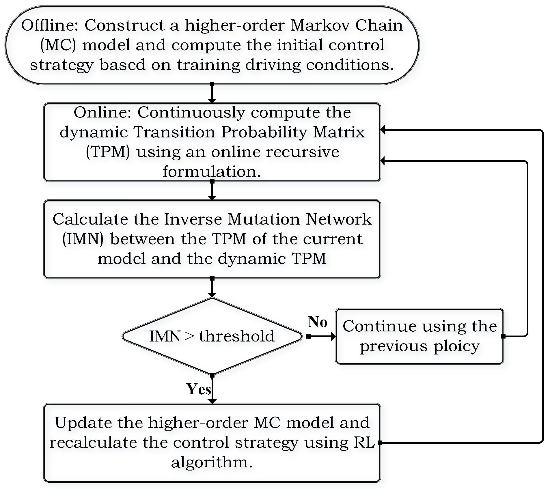
3.1.2. Online Updating of the MC Model

The transition counts in Equation (9) can be swapped out for transition frequencies, which can be written as follows, to enable real-time updates of transition probabilities:

$$\begin{array}{c}\hfill q_{kj}^i={\displaystyle \frac{C_{kj}^i/L}{C_k^i/L}}={\displaystyle \frac{F_{kj}^i\left(L\right)}{F_k^i\left(L\right)}}={\displaystyle \frac{\frac{1}{L}{\displaystyle \sum _{t=1}^L}{f}_{kj}^i\left(t\right)}{\frac{1}{L}{\displaystyle \sum _{t=1}^L}{f}_k^i\left(t\right)}}\end{array}$$

(10)

where L is the time period and i is the high-order MC’s order. The transition from state $P_{dem,t-1}=k$ to state $P_{dem,t}=j$ is represented by $f_{kj}^i\left(t\right)$, and the transitions beginning from state $P_{dem,t-1}=k$ are represented by $f_k^i\left(t\right)$. $f_{kj}^i\left(t\right)$ or $f_k^i\left(t\right)$ = 1 if the corresponding transition takes place or begins; if not, it equals 0. The average frequencies of $f_{kj}^i\left(t\right)$ and $f_k^i\left(t\right)$ are $F_{kj}^i\left(L\right)$ and $F_k^i\left(L\right)$, respectively.

Building on this, the following recursive formula may be used to determine the average frequency:

$$\begin{array}{c}\hfill \left\{\begin{array}{cc}{F}_{kj}^i\left(L\right)\hfill & ={\displaystyle \frac{1}{L}}\sum _{t=1}^L{f}_{kj}^i\left(t\right)={\displaystyle \frac{1}{L}}[(L-1)F_{kj}^i(L-1)+f_{kj}^i\left(L\right)]\hfill \\ \hfill & =F_{kj}^i(L-1)+{\displaystyle \frac{1}{L}}[f_{kj}^i\left(L\right)-F_{kj}^i(L-1)]\hfill \\ \hfill & =(1-\phi )f_{kj}^i(L-1)+\phi F_{kj}^i(L-1)\hfill \\ F_k^i\left(L\right)\hfill & =(1-\phi )f_k^i(L-1)+\phi F_k^i(L-1)\hfill \end{array}\right.\end{array}$$

(11)

where $\phi =1/L$. The decay factor $\phi$ is swapped out for a constant $\phi \in (0,1)$ in order to dynamically modify the weight of historical data through exponential decay. This parameter, which regulates the model’s update pace, is known as the forgetting factor.

The transition probabilities can then be calculated using the online recursive method that is displayed below:

$$\begin{array}{c}\hfill q_{kj}^i={\displaystyle \frac{F_{kj}^i\left(L\right)}{F_k^i\left(L\right)}}={\displaystyle \frac{=(1-\phi )f_{kj}^i(L-1)+\phi F_{kj}^i(L-1)}{=(1-\phi )f_k^i(L-1)+\phi F_k^i(L-1)}}\end{array}$$

(12)

The introduced matrix norm (IMN) is used to measure the similarity between two MC models and to decide whether to update the MC model and energy management strategy dynamically. It is clear that a higher difference between the two TPMs is indicated by a larger IMN value. Consequently, the difference between TPMs may be quantified using the scalar IMN.

$$\begin{array}{cc}\hfill IMN(Q\Vert Q^{\prime })& ={∥Q-Q^{\prime }∥}_2=\underset{1\le i\le n}{max}\left|{\epsilon }_i(Q-Q^{\prime })\right|\hfill \\ \hfill & =\underset{1\le i\le n}{max}\sqrt{{\epsilon }_i\left[{(Q-Q^{\prime })}^T(Q-Q^{\prime })\right]}\hfill \end{array}$$

(13)

where ${\epsilon }_i(Q-Q^{\prime })$ represents the eigenvalues of matrix $(Q-Q^{\prime })$, and $\mu$ is the threshold. Once the IMN exceeds $\mu$, the high-order MC model is updated by recalculating the model. Additionally, the control strategy is recomputed based on the new model.

$$\begin{array}{c}\hfill \sum _{i=1}^h{\lambda }_{i}IMN(Q_i\Vert Q_i^{\prime })>\mu \end{array}$$

(14)

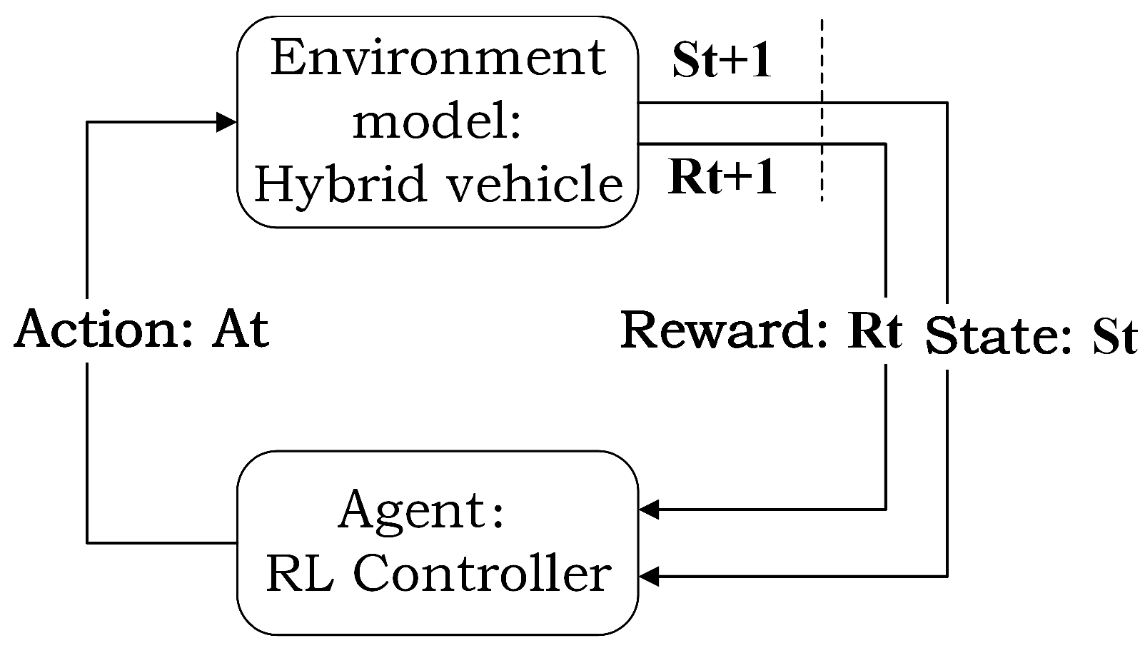
3.2. Reinforcement Learning Approach

Reinforcement learning agents optimize their behaviors based on experience gained by interacting with a model, which consists of a sequence of samples of states, actions, and rewards, or the actual world to maximize the long-term cumulative reward [21]. Model-based reinforcement learning (MBRL), which involves learning from a simulated experience using a model, and model-free reinforcement learning (MFRL), which involves learning from actual experience in the environment, are the two main categories of reinforcement learning.

The two primary components of MBRL are an RL agent that contains the control policy and an RL model that replaces the actual environment. The core mechanism of MBRL is the agent–model interaction, as shown in Figure 2. At each time step, the agent receives a state $S_t$ from the model and chooses an action $A_t$ based on this state; after executing action $A_t$, the model changes to a new state $S_{t+1}$ and produces a reward R that is given to the agent; at the same time, the agent iteratively updates its policy using the quadruple $(S_t,A_t,R_t,S_{t+1})$. The quadruple’s elements alternate until the terminal state is attained, completing the learning process.

The actual vehicle’s sensors are used to generate the states in model-free reinforcement learning. Obtaining enough data for the RL algorithm to converge can take a lot of time because the sampling time is limited. The needs of online learning can be satisfied by model-based reinforcement learning, which uses a higher-order Markov chain (MC) model to simulate state transitions.

In a traditional first-order Markov Chain model, the likelihood of $s_{t+1}$ is independent of prior states and actions, relying solely on $s_t$ and $a_t$. This assumption can lead to significant discrepancies in various engineering applications. To reduce model bias, a kth-order Markov chain model, considering states $s_{t-h+1},\dots ,s_t$ and actions $a_t$, is proposed. The probability is expressed as follows:

$$\begin{array}{c}\hfill p(s_{t+1}\mid s_1,a_1,\dots ,s_t,a_t)=p(s_{t+1}\mid s_{t-h+1},\dots ,s_t,a_t)\end{array}$$

(15)

where $p(s_{t+1}\mid s_{t-h+1},\dots ,s_t,a_t)$ is the transition probability via action $a_t$ from state $s_{t-h+1},\dots ,s_t$ to state $s_{t+1}$. It is possible to express the transition probability as $p(s_{t+1}\mid \overline{s_{h-t}},a_t)$ by defining the state $s_{t-h+1},\dots ,s_t$ as $\overline{s_{h-t}}$. Given a weight coefficient of ${\beta }_1,{\beta }_2>0$, the reward function, state variables and control variables can be expressed as follows:

$$\begin{array}{cc}\hfill r\in \mathbf{R}& =\left\{-{\dot{m}}_f-{\beta }_1{(\Delta SOC)}^2-{\beta }_2{(\Delta n_e)}^2\right\}\hfill \\ \hfill \mathbf{S}& =\left\{P_{\mathrm{dem}},\mathrm{SOC}\right\}\hfill \\ \hfill \mathbf{A}& =\left\{n_e,T_g\right\}\hfill \end{array}$$

(16)

The reward for a single time step t is denoted by $R_t$, and the long-term reward is measured by $G_t$, which is the long-term return and is defined recursively as follows:

$$\begin{array}{c}\hfill G_t=\sum _{k=0}^{\infty }{\gamma }^k{R}_{t+k}=R_t+\gamma (R_{t+1}+\gamma R_{t+2}+\dots )=R+\gamma G_{t+1}\end{array}$$

(17)

The mapping from states to the likelihood of choosing each potential course of action is called policy $\pi$. The expected return beginning from state s, following policy $\pi$, and taking action a is defined by the action value $q_{\pi }(s,a)$:

$$\begin{array}{cc}\hfill q_{\pi }(s,a)& ={\mathrm{E}}_{\pi }\left[G_t\mid S_t=s,A_t=a\right]\hfill \end{array}$$

(18)

Additionally, in the hth-order Markov chain (MC) model, the action value function’s recursive version can be written as follows:

$$\begin{array}{cc}\hfill q_{\pi }(s_t,a_t)& ={\mathrm{E}}_{\pi }\left[R_t+\gamma G_{t+1}\mid S_t=s_t,A_t=a_t\right]\hfill \\ \hfill & =R_t+\gamma \sum _{s_{t+1}\in \mathbf{S}}p(s_{t+1}\mid {\overline{s}}_{h-t},a_t){\mathrm{E}}_{\pi }\left[G_{t+1}\mid S_t=s_t\right]\hfill \\ \hfill & =R_t+\gamma \sum _{s_{t+1}\in \mathbf{S}}p(s_{t+1}\mid {\overline{s}}_{h-t},a_t)\sum _{a_{t+1}\in \mathbf{A}}\pi (a_{t+1}\mid s_{t+1})\hfill \\ \hfill & {\mathrm{E}}_{\pi }\left[G_{t+1}\mid S_{t+1}=s_{t+1},A_{t+1}=a_{t+1}\right]\hfill \\ \hfill & =R_t+\gamma \sum _{s_{t+1}\in \mathbf{S}}p(s_{t+1}\mid {\overline{s}}_{h-t},a_t)\sum _{a_{t+1}\in \mathbf{A}}\pi (a_{t+1}\mid s_{t+1})q_{\pi }(s_{t+1},a_{t+1})\hfill \end{array}$$

(19)

Additionally, the maximum action value function across all policies is the optimal action value function $q_{*}(s_t,a_t)$, and its recursive version is provided by the following:

$$\begin{array}{cc}\hfill q_{*}(s,a)& =\underset{\pi }{max}{q}_{\pi }(s,a)\hfill \\ \hfill q_{*}(s_t,a_t)& =R_t+\gamma \sum _{s_{t+1}\in \mathbf{S}}p(s_{t+1}\mid {\overline{s}}_{h-t},a_t)\underset{a_{t+1}}{max}{q}_{*}(s_{t+1},a_{t+1})\hfill \end{array}$$

(20)

The optimal policy ${\pi }^{*}$ can be derived by taking the maximum action value, assuming that the action value $q(s,a)$ is known:

$${\pi }_{*}\left(a\right|s)=\left\{\begin{array}{cc}1\hfill & \mathrm{if}a=arg\underset{a\in A}{max}{q}_{*}(s,a)\hfill \\ 0\hfill & \mathrm{otherwise}\hfill \end{array}\right.$$

(21)

An estimate of $q_{*}(s_t,a_t)$, represented as $Q_{*}(S_t,A_t)$, can be used in place of the optimal action value function in cases where the genuine optimal action-value function is unknown. The difference between the estimate of the optimal action-value function and a more precise estimate $R_t+\gamma Q(S_{t+1},A_{t+1})$ is used in the Q-learning method to update the estimate $Q_{*}(S_t,A_t)$. This difference can be represented as follows:

$$\begin{array}{cc}\hfill Q(S_t,A_t)& ⟵Q(S_t,A_t)+\alpha [R_t+\gamma Q(S_{t+1},A_{t+1})-Q(S_t,A_t)]\hfill \end{array}$$

(22)

where the learning rate parameter is denoted by $\alpha$. After every change from one state-action pair $(s_t,a_t)$ to another, this update is carried out. The action selection for the subsequent time step in the Q-learning process is decided as follows:

$$\begin{array}{c}\hfill A_{t+1}=\arg {\max }_{a\in A}Q(S_{t+1},a)\end{array}$$

(23)

The policy $\pi$ with regard to Q is $ϵ$-greedy, as follows:

$$a=\left\{\begin{array}{ll}\arg \underset{a}{max}Q(s,a)\hfill & \mathrm{probability}1-ϵ\hfill \\ \mathrm{random}(a\in A)\hfill & \mathrm{probability}ϵ\hfill \end{array}\right.$$

(24)

3.3. Adaptive Energy Management Strategy

An adaptive energy management strategy based on reinforcement learning is proposed by combining the aforementioned online-updated Markov chain model with the concepts of model-based reinforcement learning. This approach can significantly improve the performance of control strategies. Offline, training driving conditions are used to build a higher-order MC model, and the MBRL method is used to calculate the starting policy based on the model. Online, statistical information from real driving conditions are gathered using the recursive Transition Probability Matrix method, and the difference between the real-time TPM and the TPM linked to the current applied policy is assessed using IMN. In order to continuously adjust to the constantly shifting driving conditions, the higher-order Markov chain model is updated after the value surpasses a predetermined threshold $\mu$. The control strategy is then re-learned using MBRL based on the updated higher-order MC model. Furthermore, the TPM at the time of update is saved for comparison with the updated dynamic TPM. Figure 3 shows the process of the adaptive energy management system.

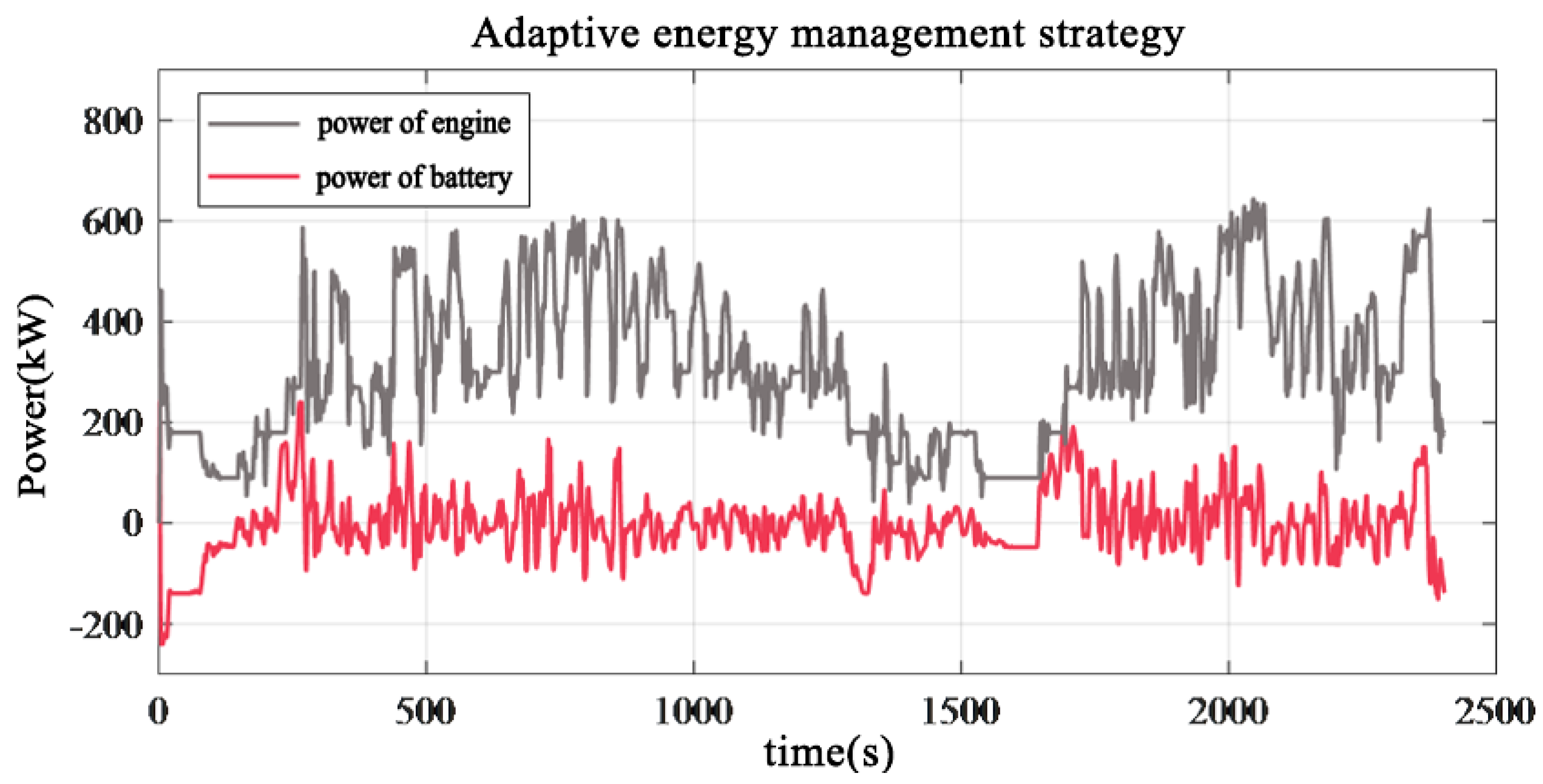
4. Simulation and Validation

To validate the effectiveness of the proposed adaptive energy management strategy, a hybrid electric vehicle model is developed in MATLAB/Simulink (version 2021b), and simulations are conducted with the proposed strategy. The proposed strategy is compared with both rule-based and conventional Q-learning-based strategies under off-road driving conditions. For Q-learning, the training driving conditions consist of the CHTC (China Heavy Truck Cycle) for road vehicles; whereas, for online reinforcement learning, CHTC is utilized solely for constructing the initial MC model and training the initial strategy. Figure 4 illustrates the off-road driving condition used, which is a high-speed driving scenario on a gravel road with comparatively minimal fluctuations in slope and road resistance coefficient. Furthermore, none of the three energy management systems take into account the off-road scenario.

Throughout the simulation process, the threshold for the induced matrix norm is set at 0.1, with a time interval of 200 s. This implies that the dynamic TPM is compared and updated with the TPM in use every 200 s. As illustrated in Figure 5, the value of IMN gradually increases over time, indicating the progressive accumulation of discrepancies between the TPM being utilized and the TPM updated with the actual driving cycles. This suggests that the previously established higher-order MC model is increasingly unable to adapt to the real driving conditions. When the IMN exceeds the threshold, this discrepancy is mitigated through updating the TPM.

The power distribution between the engine–generator set and the battery for the three strategies is depicted in Figure 6, Figure 7 and Figure 8. Under the rule-based strategy, the power of the engine and battery sometimes fluctuates frequently and abruptly, and there are instances where the power regulation relies solely on the battery, failing to fully utilize the engine’s capacity for regulation. This strategy lacks adaptability to off-road conditions compared with the online reinforcement learning strategy. Simultaneously, as indicated in Figure 5, the adaptive online reinforcement learning strategy updates the TPM at 400 s. Prior to this update, the power distribution between the engine–generator set and the battery for the online reinforcement learning strategy is identical to that of the conventional Q-learning strategy, due to consistent parameters. However, after 400 s, the online reinforcement learning strategy updates its TPM, and a significant divergence in power distribution between the two strategies begins to emerge. The update of TPM signifies that the parameters in the original reinforcement learning strategy are no longer suitable for the current off-road conditions. Consequently, in the Q-learning strategy, after 400 s, both the engine and battery power fluctuations become overly frequent and severe. In such circumstances, the engine–generator set is unable to maintain a stable operating state, and the battery frequently charges and discharges at maximum power, which has a substantial impact on battery life, engine operation stability, and fuel economy. In contrast, the updated online reinforcement learning strategy is able to maintain stable variations in engine power within the range of 200–600 kW, and the battery’s charging and discharging power fluctuates within a small margin of 200 kW. Compared with the conventional Q-learning strategy, the power distribution is more reasonable, and the strategy update allows for adaptation to the driving conditions.

Figure 9 shows the power battery’s State of Charge (SOC) for the three techniques. It is clear that the rule-based strategy is ineffective in keeping the battery’s state of charge stable. The battery’s SOC varies a lot over the driving cycle; at its highest, it surpasses 0.8, which is far greater than the SOC reference value. This indicates that the rule-based approach cannot effectively regulate the SOC. In a similar vein, the Q-learning-based strategy also fails to maintain the battery’s SOC as it is not able to adjust to off-road circumstances. Particularly in the 700–1500 s phase, the SOC experiences a substantial decrease followed by a sharp increase, and the final SOC value deviates significantly from the reference SOC value, approaching the lower limit of the set value. In contrast, the online reinforcement learning strategy maintains the battery’s SOC within the range of 0.6–0.7 throughout the entire driving cycle, and the final SOC is close to the 0.6 reference SOC. This indicates that the strategy retains a good level of control over SOC variations, even in off-road environments.

The operational conditions of the engine under the three strategies are illustrated in Figure 10. It can be observed that, under the online reinforcement learning strategy, the engine’s operating points are concentrated around the optimal engine operation curve, predominantly distributed within the range of fuel consumption less than 300 g/kWh, which is indicative of a good fuel economy. In contrast, under the conventional Q-learning-based strategy, the engine’s operating points are more dispersed, located further away from the optimal engine operation curve, and there is a significant distribution in the high fuel consumption range. This demonstrates that the traditional Q-learning-based energy management strategy does not effectively enhance the vehicle’s fuel economy in off-road conditions. Under the rule-based strategy, the engine’s operating points are mainly concentrated in two regions: 230–250 g/kWh and 260–270 g/kWh, with a scattered distribution in other areas, but the operating points do not focus on the optimal engine operation curve.

The final SOC, equivalent fuel consumption, and fuel economy for each of the three techniques are also shown in

Table 2. Results of the energy management.

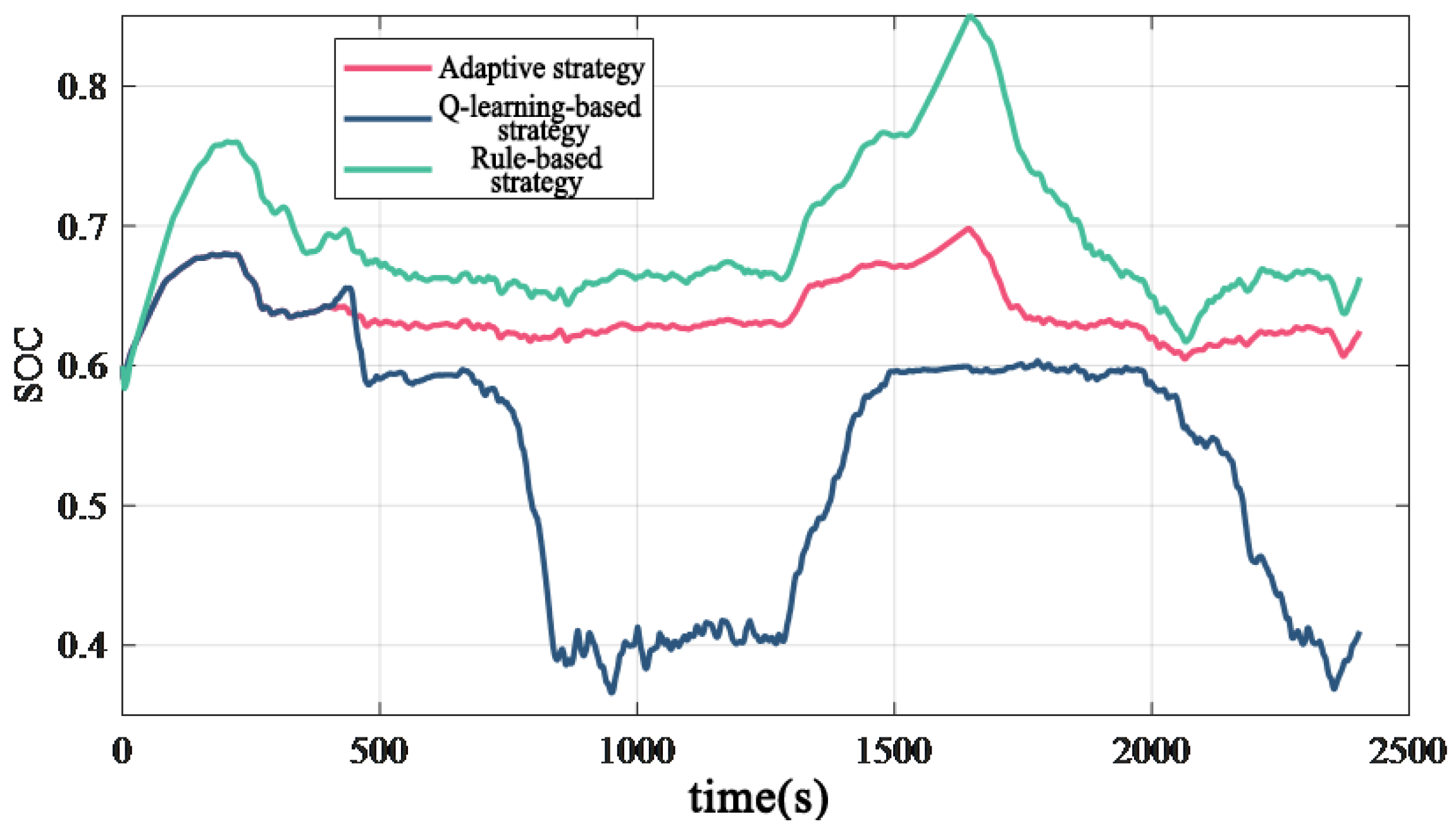
Strategy	Final SOC	Equivalent Fuel Consumption (L)	Relative Reduction (%)
adaptive strategy	0.625	62.32	100
Q-learning-based strategy	0.410	67.49	92.3
rule-based strategy	0.663	66.52	93.7

. It is evident that the online reinforcement learning method suggested in this study lowers the equivalent fuel consumption by 7.66% in comparison with the rule-based strategy and the traditional Q-learning-based strategy. It also shows improved control over the final SOC.

Future work will focus on the real-time application of the proposed strategy, including hardware-in-the-loop (HIL) testing and experimental validation, to further evaluate its performance under practical conditions.

5. Conclusions

In order to improve the RL-based energy management strategy’s adaptability while preserving real-time performance, this research proposes an adaptive energy management strategy appropriate for off-road conditions. The following are the particular conclusions:

(1) A model-based adaptive reinforcement learning algorithm is proposed. A high-order Markov chain model is utilized to characterize the power consumption in off-road conditions while taking the real-time requirement into account. Additionally, the strategy is conditionally updated online depending on the changes in the Markov chain as a criterion to increase its adaptability in off-road conditions.

(2) The suggested adaptive energy management strategy is contrasted and verified with the traditional Q-learning-based strategy and the rule-based strategy using simulation analysis conducted in off-road circumstances. In comparison with the conventional Q-learning approach, the results show that the adaptive energy management strategy can lower fuel consumption by 7.66% and better adjust to off-road conditions.

References

- Zhu, Y.; Li, X.; Liu, Q.; Li, S.; Xu, Y. Review article: A comprehensive review of energy management strategies for hybrid electric vehicles. Mech. Sci. 2022, 13, 147–188. [Google Scholar] [CrossRef]
- Ali, A.M.; Moulik, B.; Soffker, D. Intelligent Real-Time Power Management of Multi-Source HEVs Based on Driving State Recognition and Offline Optimization. IEEE Trans. Intell. Transp. Syst. 2023, 24, 247–257. [Google Scholar] [CrossRef]
- Maghfiroh, H.; Wahyunggoro, O.; Cahyadi, A.I. Energy Management in Hybrid Electric and Hybrid Energy Storage System Vehicles: A Fuzzy Logic Controller Review. IEEE Access 2024, 12, 56097–56109. [Google Scholar] [CrossRef]
- Jiang, F.; Yuan, X.; Hu, L.; Xie, G.; Zhang, Z.; Li, X.; Hu, J.; Wang, C.; Wang, H. A comprehensive review of energy storage technology development and application for pure electric vehicles. J. Energy Storage 2024, 86, 111159. [Google Scholar] [CrossRef]
- Nguyen, C.T.P.; Nguyen, B.H.; Trovao, J.P.F.; Ta, M.C. Optimal Energy Management Strategy Based on Driving Pattern Recognition for a Dual-Motor Dual-Source Electric Vehicle. IEEE Trans. Veh. Technol. 2024, 73, 4554–4566. [Google Scholar] [CrossRef]
- Xiao, R.; Liu, B.; Shen, J.; Guo, N.; Yan, W.; Chen, Z. Comparisons of energy management methods for a parallel plug-in hybrid electric vehicle between the convex optimization and dynamic programming. Appl. Sci. 2018, 8, 218. [Google Scholar] [CrossRef]
- Xu, N.; Kong, Y.; Yan, J.; Zhang, Y.; Sui, Y.; Ju, H.; Liu, H.; Xu, Z. Global optimization energy management for multi-energy source vehicles based on “Information layer—Physical layer—Energy layer—Dynamic programming” (IPE-DP). Appl. Energy 2022, 312, 118668. [Google Scholar] [CrossRef]
- Jinquan, G.; Hongwen, H.; Jianwei, L.; Qingwu, L. Real-time energy management of fuel cell hybrid electric buses: Fuel cell engines friendly intersection speed planning. Energy 2021, 226, 120440. [Google Scholar] [CrossRef]
- Li, Q.; Yang, H. Evaluation of two model predictive control schemes with different error compensation strategies for power management in fuel cell hybrid electric buses. J. Energy Storage 2023, 72, 108148. [Google Scholar] [CrossRef]
- Wu, W.; Luo, J.; Zou, T.; Liu, Y.; Yuan, S.; Xiao, B. Systematic design and power management of a novel parallel hybrid electric powertrain for heavy-duty vehicles. Energy 2022, 253, 124165. [Google Scholar] [CrossRef]
- Liu, T.; Wang, B.; Yang, C. Online Markov Chain-based energy management for a hybrid tracked vehicle with speedy Q-learning. Energy 2018, 160, 544–555. [Google Scholar] [CrossRef]
- Liu, R.; Wang, C.; Tang, A.; Zhang, Y.; Yu, Q. A twin delayed deep deterministic policy gradient-based energy management strategy for a battery-ultracapacitor electric vehicle considering driving condition recognition with learning vector quantization neural network. J. Energy Storage 2023, 71, 108147. [Google Scholar] [CrossRef]
- Wang, D.; Mei, L.; Xiao, F.; Song, C.; Qi, C.; Song, S. Energy management strategy for fuel cell electric vehicles based on scalable reinforcement learning in novel environment. Int. J. Hydrogen Energy 2024, 59, 668–678. [Google Scholar] [CrossRef]
- Ibrahim, M.; Jemei, S.; Wimmer, G.; Hissel, D. Nonlinear autoregressive neural network in an energy management strategy for battery/ultra-capacitor hybrid electrical vehicles. Electr. Power Syst. Res. 2016, 136, 262–269. [Google Scholar] [CrossRef]
- Lu, Z.; Tian, H.; Sun, Y.; Li, R.; Tian, G. Neural network energy management strategy with optimal input features for plug-in hybrid electric vehicles. Energy 2023, 285, 129399. [Google Scholar] [CrossRef]
- Huo, D.; Meckl, P. Power Management of a Plug-in Hybrid Electric Vehicle Using Neural Networks with Comparison to Other Approaches. Energies 2022, 15, 5735. [Google Scholar] [CrossRef]
- Sun, H.; Fu, Z.; Tao, F.; Zhu, L.; Si, P. Data-driven reinforcement-learning-based hierarchical energy management strategy for fuel cell/battery/ultracapacitor hybrid electric vehicles. J. Power Sources 2020, 455, 227964. [Google Scholar] [CrossRef]
- Lian, R.; Peng, J.; Wu, Y.; Tan, H.; Zhang, H. Rule-interposing deep reinforcement learning based energy management strategy for power-split hybrid electric vehicle. Energy 2020, 197, 117297. [Google Scholar] [CrossRef]
- Xu, B.; Rathod, D.; Zhang, D.; Yebi, A.; Zhang, X.; Li, X.; Filipi, Z. Parametric study on reinforcement learning optimized energy management strategy for a hybrid electric vehicle. Appl. Energy 2020, 259, 114200. [Google Scholar] [CrossRef]
- Liu, T.; Zou, Y.; Liu, D.; Sun, F. Reinforcement learning-based energy management strategy for a hybrid electric tracked vehicle. Energies 2015, 8, 7243–7260. [Google Scholar] [CrossRef]
- Sutton, R.; Barto, A. Reinforcement Learning: An Introduction; MIT Press: Cambridge, MA, USA, 1998. [Google Scholar]