Abstract
The targets for reducing greenhouse gas emissions, combined with increased electrification and the increased use of intermittent renewable energy sources, create significant challenges in matching supply and demand within distribution grid constraints. Demand response (DR) can shift electricity demand to align with constraints, reducing peak loads and increasing the utilisation of renewable generation. In countries like Aotearoa (New Zealand), peak loads are driven primarily by the residential sector, which is a prime candidate for DR. However, traditional deterministic and stochastic models do not account for the important variability in behavioural-driven residential demand and thus cannot be used to design or optimise DR. This paper presents a behavioural agent-based model (ABM) of residential electricity demand, which is validated using real electricity demand data from residential distribution transformers owned by Powerco, an electricity distributor in Aotearoa (New Zealand). The model accurately predicts demand in three neighbourhoods and matches the changes caused by seasonal variation, as well as the effects of COVID-19 lockdowns. The Pearson correlation coefficients between the median modelled and real demand are above 0.8 in 83% of cases, and the total median energy use variation is typically within 1–4%. Thus, this model provides a robust platform for network planning, scenario analysis, and DR program design or optimisation.
1. Introduction
Energy systems around the world are changing in response to climate change [1,2]. Electricity generation from renewable sources is increasing [3,4,5] and fossil-fuel-heavy sectors are being electrified [6]. For example, electricity demand in Aotearoa (New Zealand) is expected to increase by as much as 100% by 2050 [7]. Currently, renewable generation contributes 88% of Aotearoa’s (New Zealand’s) electricity, 68% of which (60% of total) is from hydroelectric power stations [8]. The additional generation required to meet this demand is expected to be primarily provided by geothermal energy and “new renewables” [9], such as wind and solar, which are predicted to constitute between 50% and 70% of the country’s energy generation by 2025 [7,10].
While considered cornerstones of the energy transition [11,12], these changes will bring challenges [13]. Increasing electrification will increase the overall electricity demand, requiring the expansion of transmission and distribution networks. Projected electrification is also expected to disproportionately increase peak demand [14,15,16], which can further reduce the lifetime of already constrained network components [17,18]. Thus, the high rate of electrification will necessitate unprecedented investment to upgrade and repair transmission and distribution infrastructure [19]. For example, Aotearoa’s (New Zealand’s) increasing electricity demand is expected to require NZD 35 billion of power system investment per decade, of which more than 60% is for distribution infrastructure [20]. Without intervention, this spending could increase consumer energy prices and energy poverty [21,22]. Additionally, new renewables are expected to increase the issue of matching supply and demand, as generation from wind and solar is more intermittent and less dispatchable than fossil-fuel- and hydroelectric-based generation [23].
Demand response (DR, also referred to as “demand flexibility”) is the practice of consumers voluntarily adjusting their electricity demand in response to signals [24], such as increasing demand to match high supply or decreasing demand to reduce peak loads. DR is particularly important in electricity systems without external connections, which is the case for Aotearoa (New Zealand) and other islands [25]. The successful implementation of DR can increase the utilisation of intermittent renewable energy sources [26,27,28] and reduce peak demands [29,30,31], reducing energy system emissions and increasing the lifetime of network components, which can reduce infrastructure expenditure as well as increase energy security and system adequacy [32,33,34].
Residential demand is typically the largest contributor to peak electricity loads in Aotearoa (New Zealand) [35] and is considered a prime candidate for DR [36,37]. However, residential energy demand is driven largely by human desires and constrained by variable human behaviour, which is inherently unpredictable and varies with dwelling type, occupancy, and appliance characteristics [38]. Thus, successful residential DR requires an accurate understanding of occupant behaviour and the desires driving it, which inform the magnitude and nature of DR potential [39]. For example, residential energy use is influenced by economic, environmental, and energy security considerations [40,41], whose importance varies across socioeconomic and cultural factors [42,43,44]. Thus, DR programs also risk entrenching existing inequalities [45,46,47], like the unequal distribution of burdens and benefits in credit card reward programs [48].
Traditional models of energy demand employ either deterministic or stochastic models of behaviour [49,50]. Deterministic models use fixed models of behaviour, which can be directly measured or inferred from aggregate data. Deterministic methods are used to model a wide range of behaviour, including transport demand [51,52,53], household appliance use [54,55,56], and building occupancy [57,58,59]. Stochastic models randomly generate behaviour from statistical distributions, which can themselves be determined from directly measured or aggregate data. Stochastic models are also widely used, such as for appliance use [60,61,62], hot water demand [63,64,65,66], electric vehicle charging [67,68], and other residential activity patterns [69,70,71].
Both deterministic and stochastic methods are well suited to modelling large groups, where aggregate group behaviour approaches the population average from which the behaviour profiles or distributions are determined. For example, electricity demand predictions at the city or national scale often use deterministic models for long-term forecasts [72,73,74] and stochastic models for shorter-term forecasts [75,76]. However, in smaller groups, individual variability is a more important factor in defining aggregate behaviour and is not captured by either deterministic or stochastic models. More importantly, neither deterministic nor stochastic models consider the desires driving these behaviours or the other ways in which these desires can be met, so they are not well suited to modelling scenarios involving behavioural changes [39].
Conversely, agent-based models (ABMs) simulate the actions of individual agents, which are determined by behavioural distributions [77]. These behavioural distributions describe how agents act and interact as well as the variability in these behaviours, with group behaviour emerging from the aggregation of all constituent agents’ behaviour. ABMs have been used to model behaviour in financial markets [78,79,80], energy markets [81,82,83,84], electric vehicle charging [85,86,87], urban driving [88], and consumer energy and technology choices [89,90,91,92]. Additionally, their versatility allows ABMs to incorporate accurate models of a range of behaviours, influenced by their underlying drivers, making them well suited for comprehensive energy demand modelling, including accounting for variations in the factors driving energy use [39], i.e., ABMs can better incorporate individual consumers’ preferences and the variability in those preferences into their predictions of behaviour, thus facilitating a more complete understanding of the factors influencing electricity demand and offering a better method of designing DR programs to suit both electricity companies and a range of consumers.
ABMs have also been used to model residential DR. To date, these models have primarily focused on participation in electricity markets, with agents representing the market decisions made by an aggregator or smart home rather than the behaviour of individual consumers [82,84,93,94]. Other research has used ABMs to optimise the charging/discharging of residential storage systems for DR, with agents representing the decisions made by the storage systems [95]. ABMs have also been used in a small number of studies to represent the behaviour of individual consumers [96,97]. However, the energy consumption behaviour in these models is based on fixed distributions, limiting their abilities to account for sources of interpersonal variability, such as socioeconomic status and geographical location, and to model changes in behaviour.
This work presents a generalisable ABM of residential electricity demand, employing a model of occupant behaviour to predict demand in a neighbourhood, defined here as the households (typically 30–100) served by a single low-voltage distribution transformer. The modelled demand is compared with real demand in three different neighbourhoods, in two stages of validation: (i) seasonal variation between summer and winter and (ii) behavioural variation during and after lockdown restrictions in Aotearoa (New Zealand) during the COVID-19 pandemic. Energy use and behaviour are informed by demographic data from the modelled neighbourhood, ensuring the model is readily generalisable to any region for which similar data are available. Thus, the model provides a robust platform to inform network planning and assess potential DR programs, facilitating an equitable, mutually beneficial energy transition.
2. Methods
Variables are assigned to households, comprising a house and its occupants (agents). Agent decisions are made according to statistical distributions of behaviour, and agents can be in one of three states: away from home, asleep, or active (awake and at home). A flowchart describing the modelling logic is shown in Figure 1.
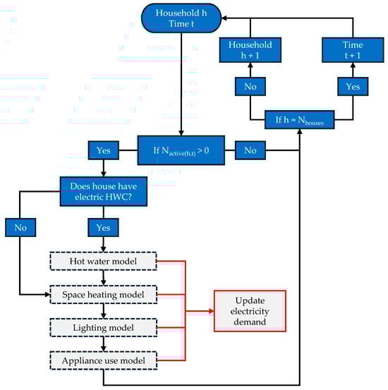
Figure 1.
Flowchart showing model logic (black arrows) and electricity information (red arrows). Nhouses is the total number of modelled households, and Nactive(h,t) is the number of active agents in house h at time t. Lighting and appliance use models are described in Section 2.2, and hot water and space heating models are described in Section 2.3.
2.1. Socioeconomic Variables
Agent incomes are assigned from a normal distribution matching NZ Census data for the modelled area [98]. Wealth coefficient of household i (WCi), a proxy of spending power, is defined:
where Ihouse,i [NZD] and Noccupants,i are the income and number of occupants of house i, and Iavg is the average individual income in Aotearoa (New Zealand) [NZD].
2.2. Behaviour, Appliances, and Lighting
Each day, agents rise from bed at twake and sleep at tsleep, both of which are generated from normal distributions matching average times in Aotearoa (New Zealand) [99,100]. Travel behaviour is modelled with four variables: number of trips per day (Ntrips), distance travelled per trip (dist), and the start and end times of each trip (tleave and tarrive), as in previous work [101]. Some agents remain at home all day and are denoted as “working from home”, the proportion of which was assumed to be 10% in this work. When working from home, agents remain in bed for an average of 1 h longer than those leaving the house during the day. These variables have been shown to be partially independent in other countries [67], but data on their interdependence in Aotearoa (New Zealand) are not available, so they were generated in this work from independent normal distributions matching travel patterns in Aotearoa (New Zealand) [102,103]. However, these methods are fully generalisable to other distributions where more refined data are available.
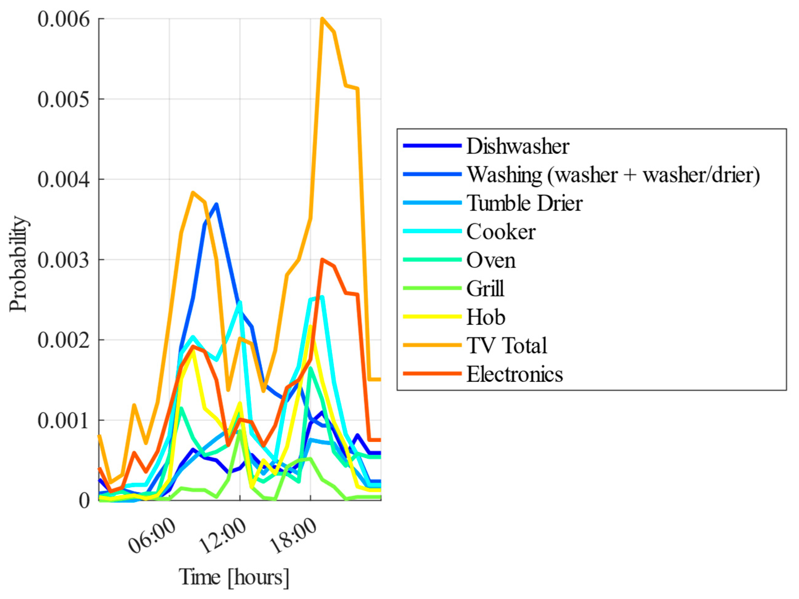
When active, agents interact with their household surroundings, using appliances according to the probability distributions in Figure 2, from profiles measured in the United Kingdom [104,105] and adjusted according to data from Aotearoa (New Zealand) [106]. Whenever agents use an appliance, the appliance draws electricity for the duration of its runtime (chosen from a normal distribution, with the average shown in Table 1). Standby (“Baseline”) loads are always running. The probability of appliance use is typically higher in winter, which is modelled with an average 20% seasonal variation (highest in June and lowest in January, for Southern Hemisphere seasons). The average electrical power and runtime for appliances are shown in Table 1.
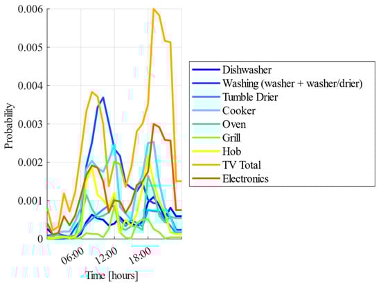
Figure 2.
Probability distributions of appliance use (baseline appliance use data from [104,105], adapted to use patterns in Aotearoa (New Zealand) according to [106]).

Table 1.
Mean appliance electrical power and runtime (from [105,106,107]). “Baseline” represents standby loads, and “Cooker” includes miscellaneous kitchen appliances.
Active agents use lighting according to outside irradiance and the number of lightbulbs in their house, with lighting use increasing with the number of active agents in a household. Lighting electricity demand for household i is generated for each timestep from the uniform distribution in the interval [0 Plight,max], where Plight,max is defined as
where Nactive,i is the number of active agents in household i, Llight is the current irradiance [Wm−2], Llight,max,i is the maximum annual irradiance in location i [Wm−2], Pbulb,i is the average power per lightbulb in household i [W], and Nbulbs,i is the number of lightbulbs in household i.
Plight,max = (Nactive,i/Noccupants,i) (1 − (Llight/Llight,max,i)) Pbulb,i Nbulbs,i
Agents can use a maximum of one appliance each minute, with independent probabilities (shown in Figure 2) for each appliance across the 24 h of a day. However, the appliances they use can continue to draw power once the agent has begun another activity, so multiple appliances can run at the same time due to the actions of a single agent. For example, an agent could switch on the hob for 30 min at 6:30 a.m and then switch on the grill for 15 min at 6:45 a.m. In such a situation, both the hob and grill would draw power until 7:00 a.m. Additionally, appliances can continue to run after agents have left their house. For example, the agent could turn on their washing machine for 60 min at 7:15 a.m. If they then leave the house at 7:45 a.m, the washing machine continues to run for 30 min after their departure.
2.3. Space and Water Heating
Details for the modelled buildings were not available, so the buildings in this work were characterised by floor area, number of floors, average insulation levels, and average window-to-wall ratios, which matches the typical approaches for large-scale models without specific data [58,108,109,110]. Ages, sizes, and window-to-wall ratios were assigned from normal distributions with averages matching the modelled population, and insulation levels were assigned according to the minimum insulation requirements of the house’s build year, as shown in Table 2. However, this modelling process is fully generalisable to changes in insulation requirements and/or the distribution of insulation in houses, such as resulting from efforts to reduce peak energy demand [111].
Table 2.
Minimum insulation requirements by build year [Wm−2K−1] from the New Zealand Building Codes 1978–2021 [112]. Zones are based on climate data and territorial authority boundaries, with higher zones indicating colder climates.
The building loss coefficient for each house is defined:
where BLC is the building loss coefficient [WK−1], and Ai [m2] and Ri [Wm−2K−1] are the surface area and R value of element i, respectively. Comfort bounds for each agent are assigned at the beginning of each simulation, and household occupants randomly select a collective comfort range within individual bounds. The “heating temperature” for household i (Theat,i [K], the temperature below which occupants of household i turn on heating) is then calculated according to the wealth coefficient:
where Tmin,i [K] is the minimum preferred temperature of household i, and Theat,min [K] is the minimum temperature below which all agents turn on heating, which varies with location [106].
BLC = (Afloor/Rfloor) + (Awalls/Rwalls) + (Aroof/Rroof) + (Awindows/Rwindows)
Theat,i = Theat,min + (Tmin,i − Theat,min)WCi
Agents turn on the heater at time t if at least one occupant is active and the inside temperature (Thouse,t [K]) is below the household heating temperature. The opposite is also true for houses with an air conditioner: air conditioning is activated if at least one occupant is active and the inside temperature is above the maximum preferred temperature. Indoor temperature is then calculated according to
where Ṫhouse is the rate of change in the inside temperature [K/s], Thouse is the inside temperature [K], Pheater is the power output from internal heating [W], Toutside is the external temperature at time t [K], and HCi is the interior heat capacity of house i [J/K].
Ṫhouse = (−(Thouse − Toutside) × BLC + Pheater)/HCi
Hot water cylinders (HWCs) are the dominant form of water heating in Aotearoa (New Zealand), with 86% of houses using an electric HWC [106], though this proportion varies between neighbourhoods. For houses with an electric HWC, its size is signed according to industry-standard recommendations based on number of occupants [113]. Hot water demand profiles w generated from DHWcalc [114], with average daily demand of 50 L per person [115,116]. HWC temperatures are calculated according to a model presented in previous work [117,118]:
where THWC is the temperature of water in the HWC [K], PHWC is the power supplied by the heater element [W], QDHW is the heat loss from hot water use [W], Qloss is the heat loss from standing losses [W], ρ is the density of water [kgm−3], Cp is the specific heat of water [Jkg−1K−1], Tin is the inlet water temperature, Thouse,i,t is the internal temperature of house i at time t [K], Kloss is an empirically tuned coefficient to a first-order approximation of the thermal losses [W/K], and Kmix is a factor to account for a thermostatic valve, defined as
where Tout is the water outlet temperature [K].
THWC = (PHWC − QDHW − Qloss)/(Cp × VHWC)
QDHW = Kmix × V × Cp × ρ (THWC − Tin)
Qloss = Kloss (THWC − Thouse,i,t)
2.4. Implementation: Neighbourhoods and Validation Cases
Modelling was conducted in MATLAB R2022b. Neighbourhoods were represented with data from the relevant mesh block, representing the highest level of granularity available from Aotearoa’s (New Zealand’s) census [98]. Three neighbourhoods connected to the electricity distribution networks of Powerco (Powerco Inc., New Plymouth, Taranaki, New Zealand) were modelled. There was one neighbourhood in Ōakura, a township of 1700 residents in Taranaki, and two in Tauranga, a city of 155,000 residents in the Bay of Plenty. The neighbourhood-dependent variables are shown in Table 3, including the New Zealand Index of Socioeconomic Deprivation (NZDep), which was used with income to provide a further evaluation of socioeconomic status [119], and all model inputs are summarised in Table 4.
2.4.1. Seasonal Variation
Each neighbourhood was modelled in summer and winter (January and June, respectively). These two months represent the peak seasonal (summer and winter) temperatures and demands. The model results were compared with real loading data from Powerco’s low-voltage electricity distribution transformers in those neighbourhoods.
Each neighbourhood was simulated for each day of each month. These results provided 31 (January) and 30 (June) daily profiles of total electricity demand. Electricity demand profiles for the median, quartiles, and 90% spread (5–95%) were plotted over a single day, showing the variation across days due to meteorological conditions, temperature, and other factors. These results were compared with real demand from Powerco’s low-voltage distribution transformers in a similar 90% range (5–95%). The median actual and modelled demands were compared with Pearson correlation coefficients to assess their similarity in shape. Finally, the total median daily consumptions were also compared for each month and neighbourhood. These metrics captured the model’s ability to represent total load, typical variability, and the trajectory over a day of electricity consumption, all three of which are a minimum requirement for such a model.
2.4.2. Lockdown Variation
On 18 August 2021, Aotearoa (New Zealand) entered Alert Level 4, the nation’s highest level of pandemic restriction, and remained there for two weeks; during this period, people were required to stay at home at all times, except those required to travel for work in essential services, such as supermarkets and healthcare facilities [120]. All neighbourhoods were modelled during the 2021 lockdown period, with 100% of the agents working from home, and during the same period in 2022, during which no COVID-19 restrictions were in place. The resulting total modelled electricity demands for each neighbourhood in each period were compared with the real transformer loads in the same way as for seasonal modelling.
Table 3.
Inputs for the modelled neighbourhoods, where income deciles are calculated from the New Zealand 2018 Household Economic Survey [121], and NZDep is the New Zealand Index of Socioeconomic Deprivation, where a higher value indicates higher deprivation [119]. The proportion of residential ICPs denotes the proportion of installation control points (ICPs) connected to a transformer that are classified as “residential”.
| Neighbourhood A | Neighbourhood B | Neighbourhood C | |
|---|---|---|---|
| Number of houses Nhouses | 68 | 34 | 69 |
| Proportion residential ICPs | 94% | 97% | 100% |
| Proportion electric HWC | 72% | 46% | 72% |
| Location | Tauranga | Ōakura | Tauranga |
| Average gross income [NZD/person/year] | 23,200 (3rd decile) | 46,000 (7th decile) | 40,900 (7th decile) |
| NZDep | 8 | 4 | 5 |
| Median age | 39 years | 40 years | 51 years |
Table 4.
Summary of model inputs.
Table 4.
Summary of model inputs.
| Variable | Value | Source |
|---|---|---|
| Average annual income | , see Table 3 | |
| Number of houses | , see Table 3 | |
| Average occupant age | , see Table 3 | |
| Appliance use profiles | , see Figure 2 | |
| Appliance characteristics | , see Table 1 | |
| Mean heater power | , 5000 W | [106] |
| Proportion of houses with heat pumps | , 19% | [122,123] |
| Mean preferred temperature (max) | , 24 °C | Estimated from [106] |
| Mean preferred temperature (min) | , 16 °C | Estimated from [106] |
| Mean house age | , 40 years | [124] |
| Mean house size | , 150 m2 | [125,126] |
| Mean number of floors | , 1.5 | [125,126] |
| Story height | , 2.4 m | [125,126] |
| Mean window–wall ratio | , 0.22 | [58] |
| House insulation level | , see Table 2 | |
| Mean trips/person/day (Ntrips) | , 0.8 | [67] |
| Mean wake time (twake) | , 0700 h | [99,100] |
| Mean sleep time (tsleep) | , 2200 h | [99,100] |
| Departure and arrival time (tleave, tarrive) | , varies | [67,103] |
| Proportion working from home | , 10% (100% in lockdown) | |
| Proportion of electric HWCs | , see Table 3 | |
| Average HWC temperature setpoint (Tset) | , 62 °C | [106] |
| HWC inlet temperature (Tin) | , 15 °C | [117,118] |
| HWC outlet temperature (Tout) | , 40 °C | |
| Average HWC heater power (PHWC) | , 1500 W | [106] |
| Average HWC volume | , 150 L | [113] |
| Average hot water demand | , 50 L/person/day | [115,118] |
| Kloss | , 0.854 WK−1 | [106,117,118] |
| Timestep (dt) | , 60 s |
3. Results
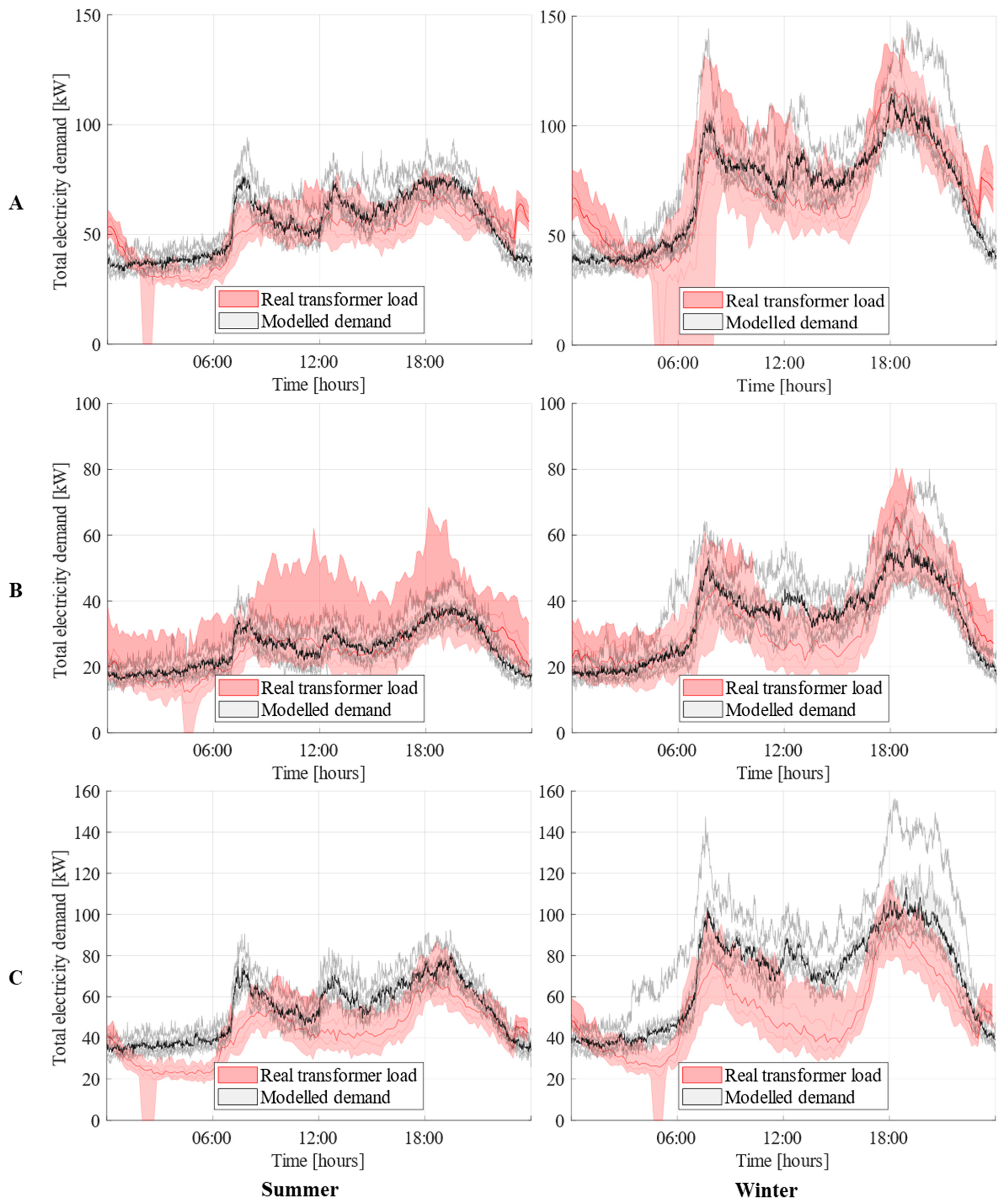
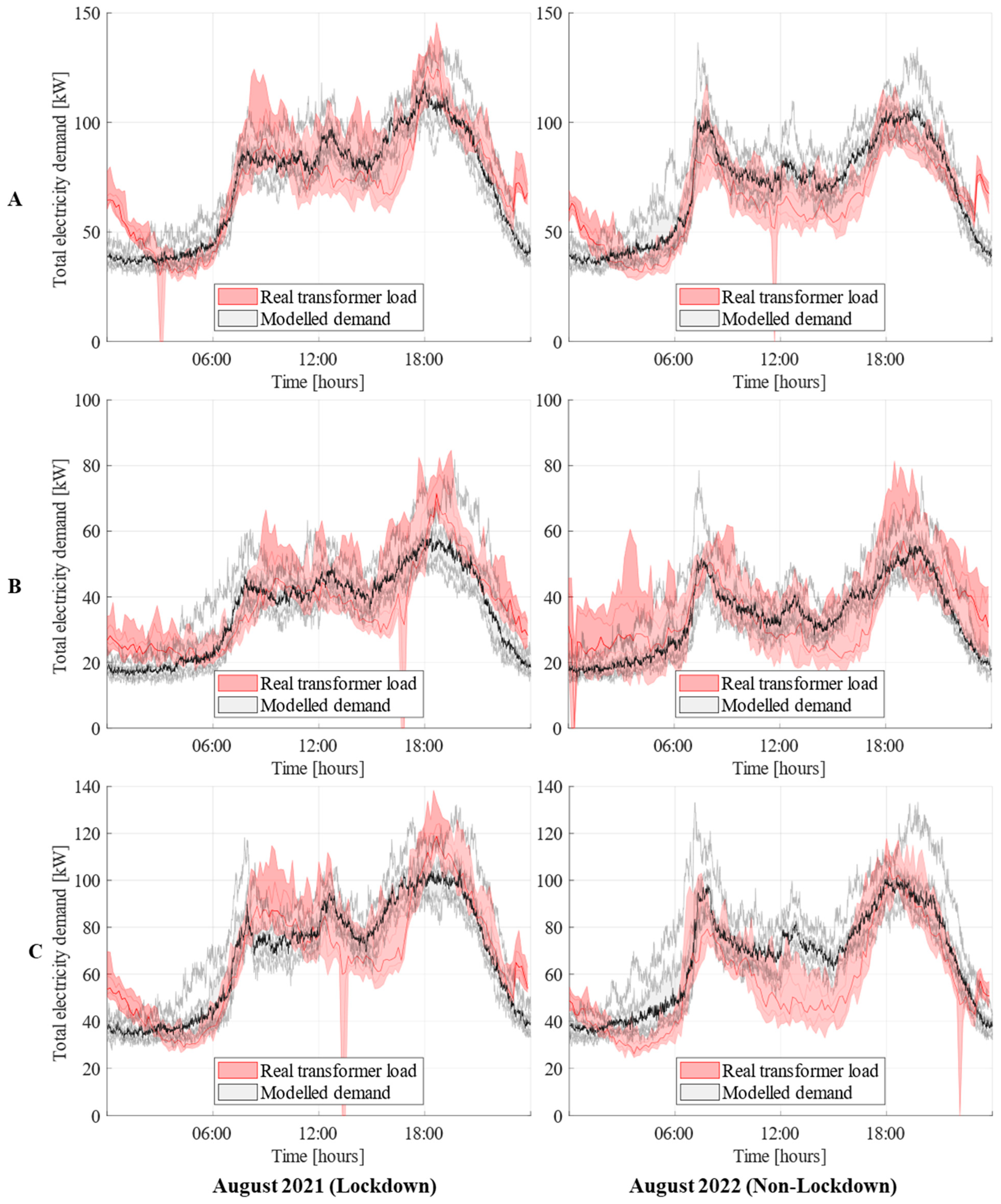
The median, quartiles, and 90% spread of the modelled demand and real transformer loading for Neighbourhoods A, B, and C during summer and winter are shown in Figure 3, and the Pearson correlation coefficients and total energy for the median demand during those periods are shown in Table 5 and Table 6, respectively. The profiles of the modelled demand and real transformer loading for Neighbourhoods A, B, and C during Aotearoa’s (New Zealand’s) August 2021 lockdown and during the same period in 2022 are shown in Figure 4, and the Pearson correlation coefficients and total energy for the median demand during those periods are shown in Table 7 and Table 8, respectively. The modelled demand had a timestep of 60 s, and real transformer loading data were provided in 10 min intervals. Zero values in the 90% spread of the transformer loading correspond to blank values for the transformer data, indicating measurement anomalies rather than real periods with no load.
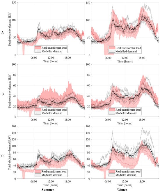
Figure 3.
Median, quartiles, and 90% spread of modelled demand (grey) and real transformer load (red) for Neighbourhoods (A–C) during summer (left) and winter (right).
Table 5.
Pearson correlation coefficients between median modelled demand and median real transformer load during summer and winter.
Table 6.
Total daily energy consumption for median modelled demand and median real transformer load during summer and winter.
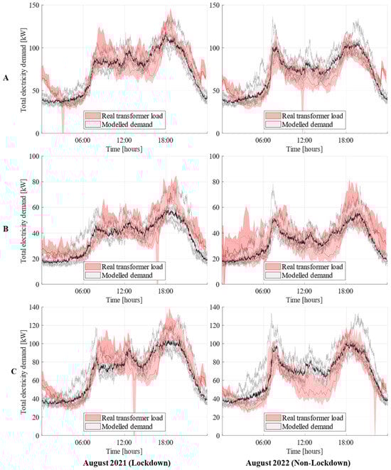
Figure 4.
Median, quartiles, and 90% spread of modelled demand (grey) and real transformer load for Neighbourhoods (A–C) during Aotearoa’s (New Zealand’s) August 2021 lockdown (left) and during the same period in 2022 (right).
Table 7.
Pearson correlation coefficients between median modelled demand and median real transformer load during Aotearoa’s (New Zealand’s) August 2021 COVID-19 lockdown and during the same period in 2022.
Table 8.
Total daily energy consumption for median modelled demand and median real transformer load during Aotearoa’s (New Zealand’s) August 2021 COVID-19 lockdown and the same period in 2022 [kWh].
4. Discussion
The presented model accurately simulated the electricity demand in all three neighbourhoods, matching the differences across seasons and due to the COVID-19 lockdowns, as shown in Figure 3 and Figure 4. The profiles of the modelled demand and real transformer load matched across all neighbourhoods and scenarios, with Pearson correlation coefficients of the median demand being between 0.66 and 0.87, as shown in Table 5 and Table 7. In all but 2 cases (of 12 total), the Pearson correlation coefficients for median electricity demand were above 0.80. Additionally, the overall energy use agreed, with a typical variation of 1–4%, between the modelled and real median energy use, as shown in Table 6 and Table 8. In all but two cases (two different cases from those for the correlation coefficient), the variation between the modelled and real median energy use was below 5%.
While the medians and quartiles of modelled and real demand were close in all cases, the 90% spread was larger for the real transformer load at lower levels of aggregation, indicating greater variability in the real world than in the model. Neighbourhood B, with only 34 houses, had a larger 90% spread in summer than Neighbourhoods A or C, as shown in Figure 3. This larger spread highlights the increased importance of individual variability in driving the aggregate behaviour of smaller groups and may reflect unmodelled behavioural changes in summer, such as vacations and seasonal celebrations. Future work would require higher-granularity data down to the household level to understand these variations and to better match the spread of the demand at lower levels of aggregation. While other models can predict electricity demand at the city or national scale, often to high levels of accuracy [67,74,76], most previous papers have not reported specific values for predictions at the neighbourhood scale, as presented in this work.
Variations in the electricity demand during Aotearoa’s (New Zealand’s) August 2021 lockdown and during the same period in 2022 were accurately captured by this model, as shown in Figure 4 and Table 7 and Table 8. By changing the proportion of agents working from home from an average of 10% to 100% to simulate the effect of travel restrictions, the model accurately matched the changes in aggregate demand for all three neighbourhoods. While data on the nature of any energy use changes during lockdown periods, or on the proportion of each neighbourhood working in essential services, are unavailable, these results suggest that such granularity is not required to represent the aggregate effects of such behavioural changes. Equally, aside from another independent validation, these results show the ability of the model to accurately capture, with no change to the model structure, the impacts of a major shift in population electricity use, which could be equal to or greater than changes resulting from a DR program.
In general, the electricity demand in summer is lower than that in winter. This seasonal variation was exhibited in all three neighbourhoods, as shown in Figure 3. The electricity demand in Aotearoa (New Zealand) is typically highest in winter, driven by increased heating loads and increased building occupancy [127,128,129]. In this model, these seasonal variations are captured in three ways: (i) higher outdoor temperatures in summer mean agents use less heating; (ii) the hot water demand profiles from DHWcalc are generated to account for 10% seasonal variation; and (iii) the profiles of appliance use probability change depending on time of year, with 20% seasonal variation between summer and winter. Thus, the assessment of seasonal variation provides a second validation of the model’s ability to account for behavioural changes.
The real transformer load data for Neighbourhoods A and C show steep increased in electricity demand around 11 p.m, which were not matched in the modelled demand, as shown in Figure 3 and Figure 4. The steepness of these increases suggests these changes may be the result of residents with time-varying electricity pricing plans, such as the cheaper overnight (11 p.m.–7 a.m.) rates offered by several electricity retail companies in Aotearoa (New Zealand), such as Octopus Energy [130], Electric Kiwi [131], and Powershop [132], to encourage the off-peak use of hot water cylinders, electric vehicles, and other appliances with deferrable loads. Thus, if this interpretation is correct, these results indicate time-varying electricity pricing plans may already be affecting demand at the low-voltage transformer level, and accounting for these effects would further increase the model’s accuracy for present-day predictions. However, the purpose of this model is to provide a platform for testing the effects of DR (in which such time-varying prices are considered), so these effects are not included in the “baseline” model presented here.
Overall, the results of this validation process suggest this model is fit for its purpose. While previous work has accurately predicted the electricity demand for large numbers of residential households, such as at the city [133,134] or national level [135], accurate neighbourhood-level modelling has previously been limited to machine learning techniques requiring previous electricity demand as an input, such as in [134,136,137]. Thus, the bottom-up nature of this modelling approach and the accuracy of the modelled demand compared with real transformer loads suggest that the approach adopted here is more versatile than current modelling techniques with similar accuracy. Furthermore, the consideration of individual behaviour and the drivers of its variability, including socioeconomic factors, means the approach presented in this work is generalisable to a range of different residential electricity consumers.
The modelling framework is also capable of incorporating alternative behavioural profiles, where data are available, and alternative technologies, such as electric vehicles, which could meet the same needs in different ways and have been the subject of previous work using a similar modelling approach [101]. Thus, this model provides a robust platform for (i) network planning, including improved demand forecasting, which could be used for “greenfield” developments for which no historical electricity demand data are available; (ii) scenario planning, such as using a travel model to assess the effects of a transition to electric vehicles, or investigating the impacts on peak loads of increased distributed generation, such as from solar panels; and (iii) DR program design, including the likely effects on energy cost, indoor temperatures, and comfort levels for people in different socioeconomic situations.
Limitations and Future Work
Validation was all conducted using data from the transformers in Powerco’s low-voltage residential distribution networks in the Taranaki and Bay of Plenty regions, achieving New Zealand Index of Deprivation (NZDep) scores of 4–8 in Table 3. Model outputs were found to be accurate in these neighbourhoods, but the data limitations meant that the performance in other neighbourhoods with greater or lower socioeconomic status was not assessed. Future work should extend model validation to include neighbourhoods in other regions and with data from other electricity distribution companies and/or with residents further towards the extremes of the deprivation index.
Variability was tested at the aggregate (neighbourhood) level, with average demand over several days. Variability also occurs in inter-household demand, as well as due to intra-household behavioural changes and/or intra-household changes in agents (e.g., travel for work, vacation). As data availability was limited to transformer-level demand profiles for privacy reasons, the ability of this model to account for these effects could not be completely assessed in this work. However, future research could use data from individual smart meters [138] or in-home appliance monitoring [139,140], among other reliable data sources, to better address these uncertainties.
As data on the building stock in each neighbourhood were not available, each neighbourhood was modelled with the same distribution of house age (mean 40 years, standard deviation 10 years). While privately rented houses are typically older and less well-insulated than those belonging to owner-occupiers in Aotearoa (New Zealand) [141], the relationships between income and house age or insulation were not quantified. However, the net effects on the electricity demand of insulation and house size, both of which decrease with decreasing income, may each other cancel out. The results presented in this work suggest that the quantification of these relationships would be beneficial for future energy modelling.
Behavioural distributions in this model are were to follow known profiles, which were derived from behaviour within wider societal constraints. For example, evening peak demands are largely the result of working hours, which restrict typical cooking times to roughly 5–8 p.m., and can be further restricted for families with young children [142]. Thus, this model should not be considered an accurate predictive tool for situations in which these wider constraints are changed or removed. For example, the model may not be able to accurately predict evening peaks if constraints around work and/or school times are considerably changed, which would impact the times during which people are home and could change the timing of different energy uses. Additionally, this model does not account for abrupt changes in behaviour, such as a shift in the heating mode [143] or the installation of distributed electricity generation [144]. Future work could thus investigate the generalisability of this model (or other agent-based approaches) to represent the behaviour of those with different constraints, such as retired people and shift workers, and assess what data are required to accurately model these changes, which could require more detailed population statistics and demographic trends [145].
Additionally, the behavioural models were derived from studies of self-reported data and directly measured appliance electricity consumption. While the sampling in these studies was intended to remove bias as much as possible, they were unlikely to include households with illicit electricity use, such as loads bypassing the electricity meter, which the occupants would not want recorded. Unaccounted-for electricity in Aotearoa (New Zealand) is typically below 3% of the total electricity use at the national level [146], but these data are not available at the low-voltage network level. Thus, discrepancies between model results and real transformer load could occur in neighbourhoods with high proportions of illicit electricity use.
The presence of distributed generation, such as behind-the-meter solar photovoltaics, was not considered in this work. While distributed generation can affect both household electricity demand and the load of the entire distribution network, the neighbourhoods used for validation in this model had very low or no distributed generation capacity. Additionally, distributed generation in Aotearoa (New Zealand) is low, with residential solar panels installed in less than 2% of households and constituting under 1% of the total electricity generation [147]. However, the modelling approach presented in this work is fully generalisable to neighbourhoods with distributed generation, and the potential impacts of solar photovoltaic uptake on residential electricity demand and distribution network loading is the subject of intended future work.
The model presented here was developed using aggregate data rather than highly granular consultation with, or surveys of, specific electricity consumers in the modelled neighbourhoods. While outside the scope of this work, future work could include such consultation with electricity consumers in a range of geographic and socioeconomic settings, which could both improve model accuracy and ensure the model is fit for purpose in its representations of the drivers of occupant behaviour and energy use. This consultation could ensure that the views and priorities of all stakeholders are represented, increasing the robustness of this modelling approach as a platform for informing future scenarios, including planning for the future modernisation of local distribution networks to better account for changing demographics and radically different energy use patterns as well as contributing to a just, equitable energy transition [148,149].
5. Conclusions
The agent-based model (ABM) presented in this work accurately captures seasonal variations in and the impact of COVID-19 lockdowns on electricity demand, with modelled demand validated with the real demand in three neighbourhoods in Aotearoa (New Zealand). With Pearson correlation coefficients for the median demand of between 0.66 and 0.87 as well as median total energy use variations typically within 1–4%, the model effectively predicts real-world demand patterns in a range of cases. The model’s ability to incorporate individual behaviour and socioeconomic factors makes it well suited for energy demand modelling and means it can be adapted to a range of geographic and socioeconomic settings as well as extended to include new technologies and behavioural changes. This generalisable model thus improves upon existing models and provides a robust platform for generating electricity demand under a range of loading scenarios, incorporating realistic energy use behaviour and the desires driving this behaviour. As such, this model can incorporate realistic behaviour and better address consumer preferences, improving network planning, scenario analysis, and demand response (DR) program design and facilitating a just, equitable energy transition. As the model’s accuracy was currently validated only for specific regions and socioeconomic contexts, future work could expand validation to other areas and incorporate more granular data, such as individual-household- or appliance-level monitoring, to enhance the model’s precision. Additionally, active engagement with electricity consumers through surveys or consultations could improve the model’s representation of behavioural drivers and ensure it incorporates the priorities and needs of a full range of electricity system stakeholders, including generators, distributors, and consumers.
Author Contributions
Conceptualisation, B.L.M.W. and J.G.C.; methodology, B.L.M.W., R.J.H., D.G. and J.G.C.; validation, B.L.M.W.; formal analysis, B.L.M.W.; investigation, B.L.M.W.; writing—original draft preparation, B.L.M.W.; writing—review and editing, B.L.M.W., R.J.H., D.G. and J.G.C.; visualisation, B.L.M.W.; supervision, R.J.H. and J.G.C. All authors have read and agreed to the published version of the manuscript.
Funding
This research received no external funding.
Data Availability Statement
Restrictions apply to the availability of the transformer loading data used for validation, which were obtained from Powerco New Zealand, and are available from the authors with the permission of Powerco. All other data in this work are available on request from the authors.
Acknowledgments
The authors would like to thank Powerco for their provision of electricity demand data to validate the models presented in this work.
Conflicts of Interest
Author R. J. Hooper was a director and employee of the company Maidstone Associates Ltd. The remaining authors declare that the research was conducted in the absence of any commercial or financial relationships that could be construed as a potential conflict of interest.
Abbreviations
The following abbreviations, variables, and subscripts are used in this manuscript:
| Abbreviation | Description | |
| ABM | Agent-based model | |
| BLC | Building loss coefficient | |
| DR | Demand response | |
| HWC | Hot water cylinder | |
| ICP | Installation control point | |
| NZDep | New Zealand Index of Socioeconomic Deprivation | |
| WC | Wealth coefficient | |
| Variable | Unit | Description |
| A | m2 | Surface area |
| BLC | WK−1 | Rate of heat loss according to temperature difference |
| Cp | Jkg−1K−1 | Specific heat of water |
| dist | m | Distance travelled per trip |
| HC | JK−1 | Internal heat capacity of house |
| I | NZD | Income |
| Kloss | WK−1 | Thermal loss coefficient from hot water cylinder |
| Kmix | Thermostatic valve mixing factor | |
| Llight | Wm−2 | Irradiance |
| Nactive | Number of active agents | |
| Nbulbs | Number of lightbulbs | |
| Nhouses | Number of houses | |
| Noccupants | Number of occupants | |
| Ntrips | Number of trips away from home per day | |
| P | W | Power |
| QDHW | W | Heat loss from hot water use |
| Qloss | W | Heat loss from HWC standing losses |
| R | Wm−2K−1 | Insulation rating |
| Theat | K | Temperature below which agents use heating |
| Thouse | K | Temperature inside house |
| THWC | K | Hot water cylinder tank temperature |
| Tin | K | Hot water cylinder inlet temperature |
| Tmax | K | Maximum preferred comfort temperature |
| Tmin | K | Minimum preferred comfort temperature |
| Tout | K | Hot water cylinder outlet temperature |
| Toutside | K | Outside ambient temperature |
| tarrive | s | Time agent arrives home |
| tleave | s | Time agent leaves home |
| twake | s | Time agent rises from bed |
| tsleep | s | Time agent goes to sleep |
| WC | Wealth coefficient | |
| ρ | kgm−3 | Density of water |
| Subscript | Description | |
| avg | Average | |
| HWC | Hot water cylinder | |
| i | House (i = 1: Nhouses) | |
| max | Maximum | |
| min | Minimum | |
| t | Time | |
References
- Cevik, S. Climate Change and Energy Security: The Dilemma or Opportunity of the Century? Environmental Economics and Policy Studies; IMF: Washington, DC, USA, 2024; pp. 1–20. [Google Scholar]
- Tarroja, B.; Mulvaney, D.; Peer, R.A.M.; Grubert, E. Evaluating the Effectiveness of Cost-Minimal Planning of Decarbonized Electricity Systems in Reducing Life Cycle Greenhouse Gas Emissions. Environ. Res. Energy 2025, 2, 015008. [Google Scholar] [CrossRef]
- Viviescas, C.; Lima, L.; Diuana, F.A.; Vasquez, E.; Ludovique, C.; Silva, G.N.; Huback, V.; Magalar, L.; Szklo, A.; Lucena, A.F.P. Contribution of Variable Renewable Energy to Increase Energy Security in Latin America: Complementarity and Climate Change Impacts on Wind and Solar Resources. Renew. Sustain. Energy Rev. 2019, 113, 109232. [Google Scholar] [CrossRef]
- Lehmann, P.; Creutzig, F.; Ehlers, M.-H.; Friedrichsen, N.; Heuson, C.; Hirth, L.; Pietzcker, R. Carbon Lock-out: Advancing Renewable Energy Policy in Europe. Energies 2012, 5, 323–354. [Google Scholar] [CrossRef]
- Olabi, A.G.; Abdelkareem, M.A. Renewable Energy and Climate Change. Renew. Sustain. Energy Rev. 2022, 158, 112111. [Google Scholar] [CrossRef]
- Sugiyama, M. Climate Change Mitigation and Electrification. Energy Policy 2012, 44, 464–468. [Google Scholar] [CrossRef]
- Ministry of Business Innovation and Employment. Electricity Demand and Generation Scenarios (EDGS); Ministry of Business Innovation and Employment: Wellington, New Zealand, 2024. [Google Scholar]
- Ministry of Business Innovation & Employment. Electricity Statistics; Ministry of Business Innovation and Employment: Wellington, New Zealand, 2023. [Google Scholar]
- Smil, V. How the World Really Works: The Science Behind How We Got Here and Where We’re Going; Viking: New York, NY, USA, 2022; ISBN 978-0593297063. [Google Scholar]
- Pimentel Pincelli, I.; Brent, A.C.; Hinkley, J.T.; Sutherland, R. Scaling up Solar and Wind Electricity: Empirical Modelling and a Disruptive Scenario for Their Deployments in Aotearoa New Zealand. J. R. Soc. N. Z. 2024, 1–23. [Google Scholar] [CrossRef]
- Haluti, I.J.; MSM, S.I.S.; Mayasri, A. Renewable Energy: A Cornerstone in The Transition Toward a Sustainable Future. JKA 2024, 1, 2. [Google Scholar] [CrossRef]
- Egerer, J.; Oei, P.-Y.; Lorenz, C. Renewable Energy Sources as the Cornerstone of the German Energiewende. In Energiewende “Made in Germany”: Low Carbon Electricity Sector Reform in the European Context; Springer Nature: Cham, Switzerland, 2018; pp. 141–172. [Google Scholar]
- Grubert, E.; Hastings-Simon, S. Designing the Mid-transition: A Review of Medium-term Challenges for Coordinated Decarbonization in the United States. Wiley Interdiscip. Rev. Clim. Change 2022, 13, e768. [Google Scholar] [CrossRef]
- Deb, S.; Tammi, K.; Kalita, K.; Mahanta, P. Impact of Electric Vehicle Charging Station Load on Distribution Network. Energies 2018, 11, 178. [Google Scholar] [CrossRef]
- Wei, M.; McMillan, C.A.; de la Rue du Can, S. Electrification of Industry: Potential, Challenges and Outlook. Curr. Sustain./Renew. Energy Rep. 2019, 6, 140–148. [Google Scholar] [CrossRef]
- Baruah, P.J.; Eyre, N.; Qadrdan, M.; Chaudry, M.; Blainey, S.; Hall, J.W.; Jenkins, N.; Tran, M. Energy System Impacts from Heat and Transport Electrification. Proc. Inst. Civ. Eng. Energy 2014, 167, 139–151. [Google Scholar] [CrossRef]
- Kwasinski, A. Quantitative Model and Metrics of Electrical Grids’ Resilience Evaluated at a Power Distribution Level. Energies 2016, 9, 93. [Google Scholar] [CrossRef]
- Susa, D.; Lehtonen, M.; Nordman, H. Dynamic Thermal Modeling of Distribution Transformers. IEEE Trans. Power Deliv. 2005, 20, 1919–1929. [Google Scholar] [CrossRef]
- IRENA. Global Energy Transformation: A Roadmap to 2050, 2019 ed.; IRENA: Abu Dhabi, United Arab Emirates, 2019. [Google Scholar]
- Boston Consulting Group. Climate Change in New Zealand: The Future Is Electric; Boston Consulting Group: Sydney, Australia, 2022. [Google Scholar]
- Faiella, I.; Lavecchia, L.; Miniaci, R.; Valbonesi, P. Household Energy Poverty and the “Just Transition”. In Handbook of Labor, Human Resources and Population Economics; Zimmermann, K.F., Ed.; Springer International Publishing: Cham, Switzerland, 2020; pp. 1–16. ISBN 978-3-319-57365-6. [Google Scholar]
- Biswas, S.; Echevarria, A.; Irshad, N.; Rivera-Matos, Y.; Richter, J.; Chhetri, N.; Parmentier, M.J.; Miller, C.A. Ending the Energy-Poverty Nexus: An Ethical Imperative for Just Transitions. Sci. Eng. Ethics 2022, 28, 36. [Google Scholar] [CrossRef]
- Joskow, P.L. Challenges for Wholesale Electricity Markets with Intermittent Renewable Generation at Scale: The US Experience. Oxf. Rev. Econ. Policy 2019, 35, 291–331. [Google Scholar] [CrossRef]
- Mathieu, J.L.; Verbič, G.; Morstyn, T.; Almassalkhi, M.; Baker, K.; Braslavsky, J.; Bruninx, K.; Dvorkin, Y.; Ledva, G.S.; Mahdavi, N. A New Definition of Demand Response in the Distributed Energy Resource Era. arXiv 2024, arXiv:2410.18768. [Google Scholar]
- Handique, A.J.; Peer, R.A.M.; Haas, J. Understanding the Challenges for Modelling Islands’ Energy Systems and How to Solve Them. Curr. Sustain./Renew. Energy Rep. 2024, 11, 95–104. [Google Scholar] [CrossRef]
- Mohseni, S.; Brent, A.C.; Kelly, S.; Browne, W.N. Demand Response-Integrated Investment and Operational Planning of Renewable and Sustainable Energy Systems Considering Forecast Uncertainties: A Systematic Review. Renew. Sustain. Energy Rev. 2022, 158, 112095. [Google Scholar] [CrossRef]
- Kirkerud, J.G.; Nagel, N.O.; Bolkesjø, T.F. The Role of Demand Response in the Future Renewable Northern European Energy System. Energy 2021, 235, 121336. [Google Scholar] [CrossRef]
- Meschede, H. Increased Utilisation of Renewable Energies through Demand Response in the Water Supply Sector—A Case Study. Energy 2019, 175, 810–817. [Google Scholar] [CrossRef]
- Rasheed, M.; Javaid, N.; Awais, M.; Khan, Z.; Qasim, U.; Alrajeh, N.; Iqbal, Z.; Javaid, Q. Real Time Information Based Energy Management Using Customer Preferences and Dynamic Pricing in Smart Homes. Energies 2016, 9, 542. [Google Scholar] [CrossRef]
- Ahmed, M.; Mohamed, A.; Homod, R.; Shareef, H. Hybrid LSA-ANN Based Home Energy Management Scheduling Controller for Residential Demand Response Strategy. Energies 2016, 9, 716. [Google Scholar] [CrossRef]
- Oprea, S.-V.; Bâra, A.; Uță, A.I.; Pîrjan, A.; Căruțașu, G. Analyses of Distributed Generation and Storage Effect on the Electricity Consumption Curve in the Smart Grid Context. Sustainability 2018, 10, 2264. [Google Scholar] [CrossRef]
- Varne, A.R.; Blouin, S.; Williams, B.L.M.; Denkenberger, D. The Impact of Abrupt Sunlight Reduction Scenarios on Renewable Energy Production. Energies 2024, 17, 5147. [Google Scholar] [CrossRef]
- Clastres, C. Smart Grids: Another Step towards Competition, Energy Security and Climate Change Objectives. Energy Policy 2011, 39, 5399–5408. [Google Scholar] [CrossRef]
- Prehoda, E.W.; Schelly, C.; Pearce, J.M. US Strategic Solar Photovoltaic-Powered Microgrid Deployment for Enhanced National Security. Renew. Sustain. Energy Rev. 2017, 78, 167–175. [Google Scholar] [CrossRef]
- Williams, B.; Bishop, D. Flexible Futures: The Potential for Electrical Energy Demand Response in New Zealand. Energy Policy 2024, 195, 114387. [Google Scholar] [CrossRef]
- Haider, H.T.; See, O.H.; Elmenreich, W. A Review of Residential Demand Response of Smart Grid. Renew. Sustain. Energy Rev. 2016, 59, 166–178. [Google Scholar] [CrossRef]
- Stephenson, J.; Ford, R.; Nair, N.-K.; Watson, N.; Wood, A.; Miller, A. Smart Grid Research in New Zealand—A Review from the GREEN Grid Research Programme. Renew. Sustain. Energy Rev. 2018, 82, 1636–1645. [Google Scholar] [CrossRef]
- Jones, R.V.; Fuertes, A.; Lomas, K.J. The Socio-Economic, Dwelling and Appliance Related Factors Affecting Electricity Consumption in Domestic Buildings. Renew. Sustain. Energy Rev. 2015, 43, 901–917. [Google Scholar] [CrossRef]
- Williams, B.; Bishop, D.; Gallardo, P.; Chase, J.G. Demand Side Management in Industrial, Commercial, and Residential Sectors: A Review of Constraints and Considerations. Energies 2023, 16, 5155. [Google Scholar] [CrossRef]
- Gyamfi, S.; Krumdieck, S. Price, Environment and Security: Exploring Multi-Modal Motivation in Voluntary Residential Peak Demand Response. Energy Policy 2011, 39, 2993–3004. [Google Scholar] [CrossRef]
- Howden-Chapman, P.; Viggers, H.; Chapman, R.; O’Dea, D.; Free, S.; O’Sullivan, K. Warm Homes: Drivers of the Demand for Heating in the Residential Sector in New Zealand. Energy Policy 2009, 37, 3387–3399. [Google Scholar] [CrossRef]
- Ruoso, A.C.; Ribeiro, J.L.D. The Influence of Countries’ Socioeconomic Characteristics on the Adoption of Electric Vehicle. Energy Sustain. Dev. 2022, 71, 251–262. [Google Scholar] [CrossRef]
- Karatasou, S.; Santamouris, M. Socio-Economic Status and Residential Energy Consumption: A Latent Variable Approach. Energy Build. 2019, 198, 100–105. [Google Scholar] [CrossRef]
- Dogan, B.; Trabelsi, N.; Khalfaoui, R.; Ghosh, S.; Shahzad, U. Role of Ethnic Diversity, Temperature Changes, and Socio-Economic Conditions for Residential Energy Use and Energy Expenditures: Evidence from the United States. Energy Build. 2022, 276, 112529. [Google Scholar] [CrossRef]
- Losi, A.; Mancarella, P.; Vicino, A. Socioeconomic Aspects of Demand Response. In Integration of Demand Response into the Electricity Chain; Wiley: Hoboken, NJ, USA, 2015; pp. 215–239. [Google Scholar]
- Brown, M.A.; Chapman, O. The Size, Causes, and Equity Implications of the Demand-Response Gap. Energy Policy 2021, 158, 112533. [Google Scholar] [CrossRef]
- Vahabi, A.R.; Latify, M.A.; Rahimiyan, M.; Yousefi, G.R. An Equitable and Efficient Energy Management Approach for a Cluster of Interconnected Price Responsive Demands. Appl. Energy 2018, 219, 276–289. [Google Scholar] [CrossRef]
- The Economist. What Donald Trump and Bernie Sanders Get Wrong about Credit Cards. The Economist, 21 November 2024.
- Herraiz-Cañete, Á.; Ribó-Pérez, D.; Bastida-Molina, P.; Gómez-Navarro, T. Forecasting Energy Demand in Isolated Rural Communities: A Comparison between Deterministic and Stochastic Approaches. Energy Sustain. Dev. 2022, 66, 101–116. [Google Scholar] [CrossRef]
- Happle, G.; Fonseca, J.A.; Schlueter, A. A Review on Occupant Behavior in Urban Building Energy Models. Energy Build. 2018, 174, 276–292. [Google Scholar] [CrossRef]
- Williams, B.; Gallardo, P.; Bishop, D.; Chase, J.G. Impacts of Electric Vehicle Policy on the New Zealand Energy System: A Retro-Analysis. Energy Rep. 2023, 9, 3871. [Google Scholar] [CrossRef]
- de Hoog, J.; Thomas, D.A.; Muenzel, V.; Jayasuriya, D.C.; Alpcan, T.; Brazil, M.; Mareels, I. Electric Vehicle Charging and Grid Constraints: Comparing Distributed and Centralized Approaches. In Proceedings of the 2013 IEEE Power & Energy Society General Meeting, Vancouver, BC, Canada, 21–25 July 2013; pp. 1–5. [Google Scholar]
- Dupont, B.; Dietrich, K.; De Jonghe, C.; Ramos, A.; Belmans, R. Impact of Residential Demand Response on Power System Operation: A Belgian Case Study. Appl. Energy 2014, 122, 1–10. [Google Scholar] [CrossRef]
- Setlhaolo, D.; Xia, X. Optimal Scheduling of Household Appliances with a Battery Storage System and Coordination. Energy Build. 2015, 94, 61–70. [Google Scholar] [CrossRef]
- Setlhaolo, D.; Xia, X. Combined Residential Demand Side Management Strategies with Coordination and Economic Analysis. Int. J. Electr. Power Energy Syst. 2016, 79, 150–160. [Google Scholar] [CrossRef]
- Luthander, R.; Widén, J.; Munkhammar, J.; Lingfors, D. Self-Consumption Enhancement and Peak Shaving of Residential Photovoltaics Using Storage and Curtailment. Energy 2016, 112, 221–231. [Google Scholar] [CrossRef]
- Hu, M.; Xiao, F. Price-Responsive Model-Based Optimal Demand Response Control of Inverter Air Conditioners Using Genetic Algorithm. Appl. Energy 2018, 219, 151–164. [Google Scholar] [CrossRef]
- Bishop, D.; Mohkam, M.; Williams, B.L.M.; Wu, W.; Bellamy, L. The Impact of Building Level of Detail Modelling Strategies: Insights into Building and Urban Energy Modelling. Eng 2024, 5, 2280–2299. [Google Scholar] [CrossRef]
- Haldi, F.; Robinson, D. The Impact of Occupants’ Behaviour on Building Energy Demand. J. Build. Perform. Simul. 2011, 4, 323–338. [Google Scholar] [CrossRef]
- Vahedipour-Dahraie, M.; Rashidizadeh-Kermani, H.; Anvari-Moghaddam, A.; Siano, P.; Catalao, J.P.S. Short-Term Reliability and Economic Evaluation of Resilient Microgrids under Incentive-Based Demand Response Programs. Int. J. Electr. Power Energy Syst. 2022, 138, 107918. [Google Scholar] [CrossRef]
- Yu, D.; Wang, J.; Li, D.; Jermsittiparsert, K.; Nojavan, S. Risk-Averse Stochastic Operation of a Power System Integrated with Hydrogen Storage System and Wind Generation in the Presence of Demand Response Program. Int. J. Hydrogen Energy 2019, 44, 31204–31215. [Google Scholar] [CrossRef]
- Yao, E.; Samadi, P.; Wong, V.W.S.; Schober, R. Residential Demand Side Management under High Penetration of Rooftop Photovoltaic Units. IEEE Trans. Smart Grid 2015, 7, 1597–1608. [Google Scholar] [CrossRef]
- Kepplinger, P.; Huber, G.; Petrasch, J. Autonomous Optimal Control for Demand Side Management with Resistive Domestic Hot Water Heaters Using Linear Optimization. Energy Build. 2015, 100, 50–55. [Google Scholar] [CrossRef]
- Kepplinger, P.; Huber, G.; Petrasch, J. Demand Side Management via Autonomous Control-Optimization and Unidirectional Communication with Application to Resistive Hot Water Heaters; ENOVA: Eisenstadt, Austria, 2014; 8p. [Google Scholar]
- Good, N.; Karangelos, E.; Navarro-Espinosa, A.; Mancarella, P. Optimization under Uncertainty of Thermal Storage-Based Flexible Demand Response with Quantification of Residential Users’ Discomfort. IEEE Trans. Smart Grid 2015, 6, 2333–2342. [Google Scholar] [CrossRef]
- Braas, H.; Jordan, U.; Best, I.; Orozaliev, J.; Vajen, K. District Heating Load Profiles for Domestic Hot Water Preparation with Realistic Simultaneity Using DHWcalc and TRNSYS. Energy 2020, 201, 117552. [Google Scholar] [CrossRef]
- Lojowska, A.; Kurowicka, D.; Papaefthymiou, G.; Van Der Sluis, L. Stochastic Modeling of Power Demand Due to EVs Using Copula. IEEE Trans. Power Syst. 2012, 27, 1960–1968. [Google Scholar] [CrossRef]
- Guo, Z.; Afifah, F.; Qi, J.; Baghali, S. A Stochastic Multiagent Optimization Framework for Interdependent Transportation and Power System Analyses. IEEE Trans. Transp. Electrif. 2021, 7, 1088–1098. [Google Scholar] [CrossRef]
- Widén, J.; Wäckelgård, E. A High-Resolution Stochastic Model of Domestic Activity Patterns and Electricity Demand. Appl. Energy 2010, 87, 1880–1892. [Google Scholar] [CrossRef]
- Vellei, M.; Martinez, S.; Le Dréau, J. Agent-Based Stochastic Model of Thermostat Adjustments: A Demand Response Application. Energy Build. 2021, 238, 110846. [Google Scholar] [CrossRef]
- Carlucci, S.; Causone, F.; Biandrate, S.; Ferrando, M.; Moazami, A.; Erba, S. On the Impact of Stochastic Modeling of Occupant Behavior on the Energy Use of Office Buildings. Energy Build. 2021, 246, 111049. [Google Scholar] [CrossRef]
- Schweizer, V.J.; Morgan, M.G. Bounding US Electricity Demand in 2050. Technol. Forecast. Soc. Change 2016, 105, 215–223. [Google Scholar] [CrossRef]
- Inglesi, R. Aggregate Electricity Demand in South Africa: Conditional Forecasts to 2030. Appl. Energy 2010, 87, 197–204. [Google Scholar] [CrossRef]
- Mirjat, N.H.; Uqaili, M.A.; Harijan, K.; Das Walasai, G.; Mondal, M.A.H.; Sahin, H. Long-Term Electricity Demand Forecast and Supply Side Scenarios for Pakistan (2015–2050): A LEAP Model Application for Policy Analysis. Energy 2018, 165, 512–526. [Google Scholar] [CrossRef]
- Alizadeh, M.; Scaglione, A.; Davies, J.; Kurani, K.S. A Scalable Stochastic Model for the Electricity Demand of Electric and Plug-In Hybrid Vehicles. IEEE Trans. Smart Grid 2014, 5, 848–860. [Google Scholar] [CrossRef]
- Trotter, I.M.; Bolkesjø, T.F.; Féres, J.G.; Hollanda, L. Climate Change and Electricity Demand in Brazil: A Stochastic Approach. Energy 2016, 102, 596–604. [Google Scholar] [CrossRef]
- de Marchi, S.; Page, S.E. Agent-Based Models. Annu. Rev. Political Sci. 2014, 17, 1–20. [Google Scholar] [CrossRef]
- Samanidou, E.; Zschischang, E.; Stauffer, D.; Lux, T. Agent-Based Models of Financial Markets. Rep. Prog. Phys. 2007, 70, 409. [Google Scholar] [CrossRef]
- Wang, L.; Ahn, K.; Kim, C.; Ha, C. Agent-Based Models in Financial Market Studies. J. Phys. Conf. Ser. 2018, 1039, 012022. [Google Scholar] [CrossRef]
- Lye, R.; Tan, J.P.L.; Cheong, S.A. Understanding Agent-Based Models of Financial Markets: A Bottom–up Approach Based on Order Parameters and Phase Diagrams. Phys. A Stat. Mech. Its Appl. 2012, 391, 5521–5531. [Google Scholar] [CrossRef]
- Shinde, P.; Amelin, M. Agent-Based Models in Electricity Markets: A Literature Review. In Proceedings of the 2019 IEEE Innovative Smart Grid Technologies—Asia (ISGT Asia), Chengdu, China, 21–24 May 2019; pp. 3026–3031. [Google Scholar]
- Dehghanpour, K.; Nehrir, M.H.; Sheppard, J.W.; Kelly, N.C. Agent-Based Modeling of Retail Electrical Energy Markets with Demand Response. IEEE Trans. Smart Grid 2016, 9, 3465–3475. [Google Scholar] [CrossRef]
- Zhou, Z.; Zhao, F.; Wang, J. Agent-Based Electricity Market Simulation with Demand Response from Commercial Buildings. IEEE Trans. Smart Grid 2011, 2, 580–588. [Google Scholar] [CrossRef]
- Xu, S.; Chen, X.; Xie, J.; Rahman, S.; Wang, J.; Hui, H.; Chen, T. Agent-Based Modeling and Simulation for the Electricity Market with Residential Demand Response. CSEE J. Power Energy Syst. 2020, 7, 368–380. [Google Scholar]
- Latifi, M.; Rastegarnia, A.; Khalili, A.; Sanei, S. Agent-Based Decentralized Optimal Charging Strategy for Plug-in Electric Vehicles. IEEE Trans. Ind. Electron. 2018, 66, 3668–3680. [Google Scholar] [CrossRef]
- Van Der Kam, M.; Peters, A.; Van Sark, W.; Alkemade, F. Agent-Based Modelling of Charging Behaviour of Electric Vehicle Drivers. J. Artif. Soc. Soc. Simul. 2019, 22, 7. [Google Scholar] [CrossRef]
- Olivella-Rosell, P.; Villafafila-Robles, R.; Sumper, A.; Bergas-Jané, J. Probabilistic Agent-Based Model of Electric Vehicle Charging Demand to Analyse the Impact on Distribution Networks. Energies 2015, 8, 4160–4187. [Google Scholar] [CrossRef]
- Benenson, I.; Martens, K.; Birfir, S. PARKAGENT: An Agent-Based Model of Parking in the City. Comput. Environ. Urban. Syst. 2008, 32, 431–439. [Google Scholar] [CrossRef]
- Rai, V.; Henry, A.D. Agent-Based Modelling of Consumer Energy Choices. Nat. Clim. Change 2016, 6, 556–562. [Google Scholar] [CrossRef]
- Hesselink, L.X.W.; Chappin, E.J.L. Adoption of Energy Efficient Technologies by Households—Barriers, Policies and Agent-Based Modelling Studies. Renew. Sustain. Energy Rev. 2019, 99, 29–41. [Google Scholar] [CrossRef]
- Rai, V.; Robinson, S.A. Agent-Based Modeling of Energy Technology Adoption: Empirical Integration of Social, Behavioral, Economic, and Environmental Factors. Environ. Model. Softw. 2015, 70, 163–177. [Google Scholar] [CrossRef]
- Silvia, C.; Krause, R.M. Assessing the Impact of Policy Interventions on the Adoption of Plug-in Electric Vehicles: An Agent-Based Model. Energy Policy 2016, 96, 105–118. [Google Scholar] [CrossRef]
- Wang, Z.; Paranjape, R. Agent-Based Simulation of Home Energy Management System in Residential Demand Response. In Proceedings of the 2014 IEEE 27th Canadian Conference on Electrical and Computer Engineering (CCECE), Toronto, ON, Canada, 4–7 May 2014; pp. 1–6. [Google Scholar]
- Golmohamadi, H.; Keypour, R.; Bak-Jensen, B.; Pillai, J.R. A Multi-Agent Based Optimization of Residential and Industrial Demand Response Aggregators. Int. J. Electr. Power Energy Syst. 2019, 107, 472–485. [Google Scholar] [CrossRef]
- Zheng, M.; Meinrenken, C.J.; Lackner, K.S. Agent-Based Model for Electricity Consumption and Storage to Evaluate Economic Viability of Tariff Arbitrage for Residential Sector Demand Response. Appl. Energy 2014, 126, 297–306. [Google Scholar] [CrossRef]
- Zhang, Z.; Jing, R.; Lin, J.; Wang, X.; van Dam, K.H.; Wang, M.; Meng, C.; Xie, S.; Zhao, Y. Combining Agent-Based Residential Demand Modeling with Design Optimization for Integrated Energy Systems Planning and Operation. Appl. Energy 2020, 263, 114623. [Google Scholar] [CrossRef]
- Wang, Y.; Lin, H.; Liu, Y.; Wennersten, R.; Sun, Q. Agent-Based Modeling of High-Resolution Household Electricity Demand Profiles: A Novel Tool for Policy Evaluating. In Proceedings of the 2017 IEEE Conference on Energy Internet and Energy System Integration (EI2), Beijing, China, 26–28 November 2017; pp. 1–6. [Google Scholar]
- Statistics New Zealand. New Zealand Census of Population and Dwellings; Statistics New Zealand: Wellington, New Zealand, 2018. [Google Scholar]
- Dorofaeff, T.F.; Denny, S. Sleep and Adolescence. Do New Zealand Teenagers Get Enough? J. Paediatr. Child. Health 2006, 42, 515–520. [Google Scholar] [CrossRef]
- Galland, B.C.; De Wilde, T.; Taylor, R.W.; Smith, C. Sleep and Pre-Bedtime Activities in New Zealand Adolescents: Differences by Ethnicity. Sleep. Health 2020, 6, 23–31. [Google Scholar] [CrossRef]
- Williams, B.; Bishop, D.; Hooper, G.; Chase, J.G. Driving Change: Electric Vehicle Charging Behavior and Peak Loading. Renew. Sustain. Energy Rev. 2024, 189, 113953. [Google Scholar] [CrossRef]
- Ministry of Transport. Vehicle Km Travelled (VKT). Available online: https://www.transport.govt.nz/statistics-and-insights/fleet-statistics/sheet/vehicle-kms-travelled-vkt-2 (accessed on 11 July 2022).
- Anderson, B.; Parker, R.; Myall, D.; Moller, H.; Jack, M. Will Flipping the Fleet F** k the Grid? In Proceedings of the 7th IAEE Asia-Oceania Conference 2020: Energy in Transition, Auckland, New Zealand, 12–15 February 2020. [Google Scholar]
- Yilmaz, S.; Firth, S.K.; Allinson, D. Occupant Behaviour Modelling in Domestic Buildings: The Case of Household Electrical Appliances. J. Build. Perform. Simul. 2017, 10, 582–600. [Google Scholar] [CrossRef]
- Kelly, J.; Knottenbelt, W. The UK-DALE Dataset, Domestic Appliance-Level Electricity Demand and Whole-House Demand from Five UK Homes. Sci. Data 2015, 2, 150007. [Google Scholar] [CrossRef]
- Isaacs, N.; Camilleri, M.; Burrough, L.; Pollard, A.; Saville-Smith, K.; Fraser, R.; Rossouw, P.; Jowett, J. Energy Use in New Zealand Households: Final Report on the Household Energy End-Use Project (Heep); BRANZ Study Report: Porirua, New Zealand, 2010; Volume 221, pp. 15–21. [Google Scholar]
- Bizzozero, F.; Gruosso, G.; Vezzini, N. A Time-of-Use-Based Residential Electricity Demand Model for Smart Grid Applications. In Proceedings of the 2016 IEEE 16th International Conference on Environment and Electrical Engineering (EEEIC), Florence, Italy, 7–10 June 2016; pp. 1–6. [Google Scholar]
- Battini, F.; Pernigotto, G.; Gasparella, A. A Shoeboxing Algorithm for Urban Building Energy Modeling: Validation for Stand-Alone Buildings. Sustain. Cities Soc. 2023, 89, 104305. [Google Scholar] [CrossRef]
- Battini, F.; Pernigotto, G.; Gasparella, A. District-Level Validation of a Shoeboxing Simplification Algorithm to Speed-up Urban Building Energy Modeling Simulations. Appl. Energy 2023, 349, 121570. [Google Scholar] [CrossRef]
- Bishop, D.; Gallardo, P.; Williams, B.L.M. A Review of Multi-Domain Urban Energy Modelling Data. Clean. Energy Sustain. 2023, 2, 10016. [Google Scholar] [CrossRef]
- Maxim, A.; Grubert, E. Highly Energy Efficient Housing Can Reduce Peak Load and Increase Safety under Beneficial Electrification. Environ. Res. Lett. 2023, 19, 014036. [Google Scholar] [CrossRef]
- Ministry of Business Innovation and Employment. New Zealand Building Code H1 Energy Efficiency Acceptable Solution H1/AS1: Energy Efficiency for All Housing, and Buildings Up to 300 M2; Ministry of Business Innovation and Employment: Wellington, New Zealand, 2021. [Google Scholar]
- HeatingForce. What Size Hot Water Cylinder Do I Need? Available online: https://heatingforce.co.uk/blog/what-size-cylinder-do-i-need/ (accessed on 11 November 2021).
- Jordan, U.; Vajen, K. DHWcalc: Program to Generate Domestic Hot Water Profiles with Statistical Means for User Defined Conditions. In Proceedings of the ISES Solar World Congress, Orlando, FL, USA, 6–12 August 2005; pp. 8–12. [Google Scholar]
- Basson, J. The Heating of Residential Sanitary Water (in Afrikaans); National Building Research Institute: Pretoria, South Africa, 1983. [Google Scholar]
- Parker, D.S.; Fairey, P.W.; Lutz, J.D. Estimating Daily Domestic Hot-Water Use in North American Homes. ASHRAE Trans. 2015, 121, 258–270. [Google Scholar]
- Bishop, D.; Nankivell, T.; Williams, B. Peak Loads vs. Cold Showers: The Impact of Existing and Emerging Hot Water Controllers on Load Management. J. R. Soc. N. Z. 2023, 1–26. [Google Scholar] [CrossRef]
- Williams, B.; Bishop, D.; Docherty, P. Assessing the Energy Storage Potential of Electric Hot Water Cylinders with Stochastic Model-Based Control. J. R. Soc. N. Z. 2023, 1–17. [Google Scholar]
- Atkinson, J.; Salmond, C.; Crampton, P.; Viggers, H.; Lacey, K. NZDep2023 Index of Socioeconomic Deprivation: Research Report; University of Otago: Wellington, New Zealand, 2024. [Google Scholar]
- Ministry of Health. Aotearoa New Zealand’s COVID-19 Elimination Strategy: An Overview; Ministry of Health: Wellington, New Zealand, 2021. [Google Scholar]
- Statistics New Zealand. Household Economic Survey (Income) 2018; Statistics New Zealand: Wellington, New Zealand, 2018. [Google Scholar]
- French, L.J. Active Cooling and Heat Pump Use in New Zealand: Survey Results; BRANZ: Porirua, New Zealand, 2008. [Google Scholar]
- Buckett, N.R. National Impacts of the Widespread Adoption of Heat Pumps in New Zealand; BRANZ: Porirua, New Zealand, 2007. [Google Scholar]
- Stats, N.Z. Housing in Aotearoa: 2020; NZ Government: Wellington, New Zealand, 2020. [Google Scholar]
- Khajehzadeh, I.; Vale, B. How House Size Impacts Type, Combination and Size of Rooms: A Floor Plan Study of New Zealand Houses. Archit. Eng. Des. Manag. 2017, 13, 291–307. [Google Scholar] [CrossRef]
- Khajehzadeh, I.; Vale, B. Large Housing in New Zealand: Are Bedroom and Room Standards Still Good Definitions of New Zealand House Size. In Proceedings of the the 9th Australasian Housing Researchers Conference, Auckland, New Zealand, 17 February 2016; The University of Auckland: Auckland, New Zealand; 2016; pp. 17–19. [Google Scholar]
- Dortans, C.; Jack, M.W.; Anderson, B.; Stephenson, J. Lightening the Load: Quantifying the Potential for Energy-Efficient Lighting to Reduce Peaks in Electricity Demand. Energy Effic. 2020, 13, 1105–1118. [Google Scholar] [CrossRef]
- Renwick, J.; Mladenov, P.; Purdie, J.; McKerchar, A.; Jamieson, D. The Effects of Climate Variability and Change upon Renewable Electricity in New Zealand. In Climate Change Adaptation in New Zealand: Future Scenarios and Some Sectoral Perspectives; New Zealand Climate Change Centre: Wellington, New Zealand, 2010; pp. 70–81. [Google Scholar]
- Dortans, C.; Anderson, B.; Jack, M. NZ GREEN Grid Household Electricity Demand Data: EECA Data Analysis (Part B) Report v2. 1; University of Otago: Dunedin, New Zealand, 2019. [Google Scholar]
- Octopus Energy. Use Your Power Wisely—The Lowdown on Our Off-Peak and Night Rates. Available online: https://octopusenergy.nz/blog/the-lowdown-on-our-off-peak-and-night-rates (accessed on 23 December 2024).
- Electric Kiwi. Power Plans. Available online: https://www.electrickiwi.co.nz/power/plans (accessed on 23 December 2024).
- Powershop. Get Shifty (Time of Use). Available online: https://www.powershop.co.nz/help/get-shifty-time-of-use/ (accessed on 23 December 2024).
- Porteiro, R.; Hernández-Callejo, L.; Nesmachnow, S. Electricity Demand Forecasting in Industrial and Residential Facilities Using Ensemble Machine Learning. Rev. Fac. Ing. Univ. Antioq. 2022, 102, 9–25. [Google Scholar] [CrossRef]
- Cai, H.; Shen, S.; Lin, Q.; Li, X.; Xiao, H. Predicting the Energy Consumption of Residential Buildings for Regional Electricity Supply-Side and Demand-Side Management. IEEE Access 2019, 7, 30386–30397. [Google Scholar] [CrossRef]
- Dilaver, Z.; Hunt, L.C. Modelling and Forecasting Turkish Residential Electricity Demand. Energy Policy 2011, 39, 3117–3127. [Google Scholar] [CrossRef]
- Jiang, Q.; Huang, C.; Wu, Z.; Yao, J.; Wang, J.; Liu, X.; Qiao, R. Predicting Building Energy Consumption in Urban Neighborhoods Using Machine Learning Algorithms. Front. Urban Rural Plan. 2024, 2, 6. [Google Scholar] [CrossRef]
- Gao, S.; Zhang, X.; Gao, L.; Zhou, Y.; Wu, T. A Novel Residential Electricity Load Prediction Algorithm Based on Hybrid Seasonal Decomposition and Deep Learning Models. SSRN 2024. [Google Scholar] [CrossRef]
- Wijaya, T.K.; Vasirani, M.; Humeau, S.; Aberer, K. Cluster-Based Aggregate Forecasting for Residential Electricity Demand Using Smart Meter Data. In Proceedings of the 2015 IEEE International Conference on Big Data (Big Data), Santa Clara, CA, USA, 29 October–1 November 2015; pp. 879–887. [Google Scholar]
- Pipattanasomporn, M.; Kuzlu, M.; Rahman, S.; Teklu, Y. Load Profiles of Selected Major Household Appliances and Their Demand Response Opportunities. IEEE Trans. Smart Grid 2013, 5, 742–750. [Google Scholar] [CrossRef]
- Cetin, K.S.; Tabares-Velasco, P.C.; Novoselac, A. Appliance Daily Energy Use in New Residential Buildings: Use Profiles and Variation in Time-of-Use. Energy Build. 2014, 84, 716–726. [Google Scholar] [CrossRef]
- Howden-Chapman, P.; Crane, J.; Keall, M.; Pierse, N.; Baker, M.G.; Cunningham, C.; Amore, K.; Aspinall, C.; Bennett, J.; Bierre, S. He Kāinga Oranga: Reflections on 25 Years of Measuring the Improved Health, Wellbeing and Sustainability of Healthier Housing. J. R. Soc. N. Z. 2024, 54, 290–315. [Google Scholar] [CrossRef]
- Nicholls, L.; Strengers, Y. Peak Demand and the ‘Family Peak’ Period in Australia: Understanding Practice (in)Flexibility in Households with Children. Energy Res. Soc. Sci. 2015, 9, 116–124. [Google Scholar] [CrossRef]
- Jose, L.; Raxworthy, M.; Williams, B.L.M.; Denkenberger, D. Be Clever or Be Cold: Repurposed Ovens for Space Heating Following Global Catastrophic Infrastructure Loss. EarthArXiv 2024. [Google Scholar] [CrossRef]
- Williams, B.; Croft, H.; Hunt, J.; Viloria, J.; Sherman, N.; Oliver, J.; Green, B.; Turchin, A.; García Martínez, J.; Pearce, J.; et al. Wood Gasification in Catastrophes: Electricity Production from Light Duty Vehicles. EarthArXiv 2025. [Google Scholar] [CrossRef]
- Cook, L. Illuminating the Intergenerational Value of Regular Population Censuses Whilst Amidst a Population Storm; Economic Policy Centre: Auckland, New Zealand, 2024. [Google Scholar]
- Electricity Authority. Unaccounted for Electricity. Available online: https://www.emi.ea.govt.nz/All/Reports/CPMJNV (accessed on 24 January 2025).
- Energy Efficiency and Conservation Authority. Solar Energy in New Zealand. Available online: https://www.eeca.govt.nz/insights/energy-in-new-zealand/renewable-energy/solar/ (accessed on 9 February 2025).
- Wang, X.; Lo, K. Just Transition: A Conceptual Review. Energy Res. Soc. Sci. 2021, 82, 102291. [Google Scholar] [CrossRef]
- Newell, P.; Mulvaney, D. The Political Economy of the ‘Just Transition’. Geogr. J. 2013, 179, 132–140. [Google Scholar] [CrossRef]

Disclaimer/Publisher’s Note: The statements, opinions and data contained in all publications are solely those of the individual author(s) and contributor(s) and not of MDPI and/or the editor(s). MDPI and/or the editor(s) disclaim responsibility for any injury to people or property resulting from any ideas, methods, instructions or products referred to in the content. |
© 2025 by the authors. Licensee MDPI, Basel, Switzerland. This article is an open access article distributed under the terms and conditions of the Creative Commons Attribution (CC BY) license (https://creativecommons.org/licenses/by/4.0/).