Gas−Hydro Coordinated Peaking Considering Source-Load Uncertainty and Deep Peaking

Abstract

Considering the power demand in high-altitude special environmental areas and the peak-regulation issues in the power system caused by the uncertainties associated with wind and photovoltaic power as well as load, a gas–hydro coordinated peak-shaving method that considers source-load uncertainty is proposed. Firstly, based on the regulation-related characteristics of hydropower and gas power, a gas−hydro coordinated operation mode is proposed. Secondly, the system operational risk caused by source-load uncertainty is quantified based on the Conditional Value-at-Risk theory. Then, the cost of deep peak shaving in connection with gas-fired power generation is estimated, and a gas−hydro coordinated peak-shaving model considering risk constraints and deep peak shaving is established. Finally, a specific example verifies that the proposed gas−hydro coordinated peak-regulation model can effectively improve the economy of the system. The total system profit increased by 36.03%, indicating that this method enhances the total system profit and achieves better peak-shaving effects.

1. Introduction

The rate of energy-structure transformation is accelerating against the background of ‘dual carbon’ targets [1]. In the face of the new market demand, in some high-altitude environmental areas, there are many problems, such as a relatively weak regional economy and industrial base, insufficient infrastructure, and high requirements for environmental protection [2]. In such special environmental areas, the lack of safe, green, sustainable, and affordable energy has been a problem hindering their development, and the construction of clean, low-carbon energy stations is a high priority, with remote areas being developed to generate electric power to allow for further development [3]. However, with the increase in the proportion of energy generated by wind and the solar grid, the uncertainties associated with wind and photovoltaic power, as well as load, place higher demands on the peak-shaving ability of the power system [4,5,6,7]. Therefore, this paper proposes a gas−hydro coordinated peaking model considering source-load uncertainty and further proposes mobilizing the initiative for gas−electric peak regulation through a deep peak-regulation compensation price mechanism, alleviating the system-peaking dilemma associated with a grid-connected wind-energy system, improving the system’s operational economy and robustness, and providing technical support for the development of new energy resources in Tibet and other special environmental areas.

To address the uncertainties associated with wind and PV-containing systems, a large number of experts have conducted research on operational risk, stochastic optimization, and robust optimization [8,9,10,11]. The impact of the hydropower output on residual load variability and system operational risk under different hydrometeorological conditions has been analyzed in the literature [12]. A multi-objective optimal scheduling model for hydro, wind, and PV has been developed and published in the literature [13]; it considers the operational risks of curtailment and outage and uses gradient hydropower to reduce the risks associated with uncertainty in wind and PV systems. A hydro−fire−optical short-term peaking multi-objective optimization model was constructed based on the risk avoidance and opportunity-seeking strategies employed in information-gap decision techniques, using hydropower as the dominant force to reduce the uncertainty associated with wind and light, and published in the literature [14]. A two-stage distributional robust optimization model for hydro–wind PV has also been developed and published in the literature [15]; this model can effectively respond to the stochasticity and instability of renewable energy sources. Monte Carlo and the roulette wheel mechanism have been used in the literature to build a multi-objective scheduling model for hydro–fire–wind PV [16], and the ε constraint method was adopted to select the Pareto solution. However, the hydropower output drops sharply under extreme drought and disaster-level weather conditions, and the uncertainty of the source load poses a more serious challenge to system operation, which requires low-carbon, flexible gas power to provide strong support; however, there has been little research on the coordination of gas and hydropower to cope with the operational risk of the system. The question of how to fully leverage the peak-shaving advantage of gas and electricity and coordinate the operation of hydropower to preserve the energy supply needs to be explored in depth.

To date, a large number of experts have studied the peak-regulation dispatching of the power system, and a peak-regulation cost distribution mechanism considering the peak-regulation demand is established in the literature [17]. It has been verified that the mechanism can reflect the different load costs and reduce the load pressure of the thermal power unit. A short-term peak-regulation model of hydropower stations is proposed in the literature [18], which can effectively improve the decision-making ability in cascade hydropower dispatching, solve the uncertainty of wind power and photovoltaics, and support the stable operation of the power grid. Considering the long-term water distribution and short-term peak-regulation demand of cascade hydropower stations, a capacity planning method has been established to help reasonably plan the capacity of renewable energy power plants [19]. In order to improve the peak-regulation capacity of the system and consider the relationship between supply and demand, a peak-regulation compensation mechanism is proposed in the literature [20], which effectively promotes joint peak regulation and wind power consumption. Demand response resources were considered to establish the combined mixed-integer linear planning (MILP) model in [21], and the example given verifies that the use of demand response means is conducive to the joint peak-regulation operation of water, fire, and electricity. Most of the above studies use hydropower or thermal power. However, the output of hydropower decreases during the dry season, and thermal power’s environmental pollution is serious, its start–stop is slow, and its climbing performance is weak; plus, it does not adapt to the “double carbon” energy scenario in China, which requires low-carbon, high-quality transformation of the situation. The gas–electric unit has low carbon emissions, fast climbing, and start and stop speed. It can coordinate with the cascade hydropower with a huge power reserve to meet the balance of power supply and demand, has cascade hydraulic coupling characteristics, and can flexibly regulate gas and electricity.

Based on the above, this paper establishes a gas–hydro coordinated peaking model considering source-load uncertainty. The main contributions are summarized as follows:

• This paper analyzes the joint operation mode of a gas–hydro coordinated model based on the regulating characteristics of gas power and hydropower;
• In this paper, we propose a method to quantify the risk of system operation caused by source-load uncertainty based on CVaR theory;
• This paper considers the model of deep peak regulation to manage source-load uncertainty and reduce abandoned water;
• Based on 1 and 2, a gas–hydro coordinated peaking model is proposed, aiming at maximizing the net profit of peak shaving with the CVaR theory and the cost of deep peak shaving, and this paper use linearization methods to manage the mixed-integer nonlinear programming model.

The organization of this paper is as follows. Section 1 introduces the gas–hydro coordinated operation model. Section 2 describes the operation risk. Section 3 describes the deep peaking of gas turbines. In Section 4, the gas–hydro coordinated peak-shaving model considering deep peak-shaving compensation for gas turbines is proposed. Section 5 reports the case study results. Section 6 concludes the paper.

2. Gas–Hydro Coordinated Operation Model

In this paper, hydropower is coordinated with gas power to implement gas–hydro coordinated peak shaving to ensure a system supply–demand balance and achieve economic operation of the system. In order to improve the rate of new energy consumption, wind power and photovoltaic are prioritized for grid-connected power generation, and the remaining load demand is met through gas–hydro coordinated peaking [22]. If the traditional scheduling method of hydropower taking the base load and gas power taking the peak load task are adopted, this will inevitably cause frequent starting and stopping of gas power units, which affects the system economy. Therefore, this paper proposes the following scheduling strategy: set the base load to be borne by gas power and hydropower in the low load time, increase reservoir storage with hydropower with seasonal regulation capability, and reduce hydropower output. In the load peak time, increase the hydropower output in response to load fluctuations by releasing water from reservoirs, smoothing the gas power output in the full cycle and reducing the frequency of gas power units starting and stopping; at the same time, due to the wind–PV and load prediction error, when the system faces a shortage of up-peaking or down-peaking, the rotating reserve capacity is reserved with gas power units with fast climbing ability, to cope with the uncertainty on both sides of the source and load and satisfy the balance of supply and demand in the power system. Through the implementation of the above scheduling strategy, hydropower and gas power are fully mobilized for coordinated peaking, which in turn matches the net load characteristics. Especially when the system is faced with extreme drought and disaster weather, the hydropower output falls sharply, which exacerbates the system’s dependence on a stable peaking power source; however, gas power can avoid the power deficit caused by the fall of the hydropower output, by responding to the system’s peaking demand and generating electricity on the grid quickly, which reduces the amount of coal power generation, improves the economy and environmental protection of the system, reduces the risk of system operation, and ensures the safe and stable operation of the system.

3. System Operation Risk Analysis

3.1. System Uncertainty Analysis

The uncertainty of the system is mainly caused by the random fluctuations of wind power, PV, and the load, and the uncertainty on both sides of the source and load can be attributed to the uncertainty of the net load after the system consumes the wind and solar output [23].

3.1.1. Load Uncertainty

The prediction error of the net load can be expressed as Equation (1).

$${\xi }_{\mathrm{L},t}=P{L}_{\mathrm{real},t}-P{L}_{f,t}$$

(1)

where $P{L}_{\mathrm{real},t}$ and $P{L}_{f,t}$ are the actual and predicted values of load at time t, respectively.

It is assumed that the short-term load forecast error follows a normal distribution with a mean of 0, and the standard deviation ${\delta }_{\mathrm{L},t}$ is taken as a percentage of the load forecast value ${\theta }_{L,t}$ [24].

3.1.2. Wind–Photovoltaic Joint Uncertainty

The prediction error of the wind power output at time period t can be expressed by the following equation:

$${\xi }_{W,t}=P{W}_{\mathrm{real},t}-P{W}_{f,t}$$

(2)

where $P{W}_{\mathrm{real},t}$ and $P{W}_{f,t}$ are the actual and predicted values of the wind power output in time period t, respectively.

Assuming that the wind power output prediction error obeys a normal distribution with mean 0, the standard deviation ${\delta }_{\mathrm{W},t}$ can be determined by the following equation:

$${\delta }_{\mathrm{W},t}=a_{\mathrm{W}}P{W}_{f,t}+b_{\mathrm{W}}P{W}_{\mathrm{N}}$$

(3)

where $P{W}_N$ is the total installed capacity of wind power; and $a_W$ and $b_W$ are the output allocation factor and the installed capacity allocation factor, respectively.

The prediction error of PV output at time period t can be expressed by the following equation:

$${\xi }_{\mathrm{V},t}=P{V}_{\mathrm{real},t}-P{V}_{f,t}$$

(4)

where $P{V}_{\mathrm{real},t}$ and $P{V}_{f,t}$ are the actual and predicted values of PV output in time period t, respectively.

Assuming that the PV output prediction error obeys a normal distribution with mean 0, the standard deviation ${\delta }_{V,t}$ can be determined by the following equation:

$${\delta }_{\mathrm{V},t}=a_{\mathrm{V}}P{V}_{f,t}+b_{\mathrm{V}}P{V}_{\mathrm{N}}$$

(5)

where $P{V}_N$ is the total installed capacity of PV; and $a_{\mathrm{V}}$ and $b_{\mathrm{V}}$ are the output allocation factor and the installed capacity allocation factor, respectively.

We define the linear combination of wind power and PV output prediction error as the wind power and PV joint prediction error, and according to the basic nature of the normal distribution, this has a normal distribution. The joint wind–PV prediction error is shown in the following equation:

$${\xi }_{un,t}={\xi }_{\mathrm{W},t}+{\xi }_{\mathrm{V},t}$$

(6)

The standard deviation of the joint wind–PV prediction error is as follows:

$${\delta }_{un,t}=\sqrt{{\delta }_{\mathrm{W},t}^2+{\delta }_{\mathrm{V},t}^2+2\mathrm{\Psi }{\delta }_{\mathrm{W},t}{\delta }_{\mathrm{V},t}}$$

(7)

where $\mathrm{\Psi }$ is Spearman’s correlation coefficient for the joint wind–PV prediction error [25], which is taken as −0.37 and −0.2 in summer and winter, respectively.

3.1.3. Net Load Uncertainty

The prediction error of the net load can be expressed by the following equation:

$${\xi }_{L,t}^{\mathrm{net}}=P{L}_{\mathrm{real},t}^{\mathrm{net}}-P{L}_{f,t}^{\mathrm{net}}$$

(8)

where $P{L}_{\mathrm{real},t}^{\mathrm{net}}$ and $P{L}_{f,t}^{\mathrm{net}}$ are the actual and predicted values of the net load for period t, respectively.

The uncertainty of the system is mainly caused by wind power, PV, and random load fluctuations. When the system consumes wind and PV power, the uncertainty on both sides of the power load can be attributed to the uncertainty of the net load [23]. The predicted values of the net load can be expressed as Equation (9).

$$P{L}_{f,t}^{\mathrm{net}}=P{L}_{f,t}-P{W}_{f,t}-P{V}_{f,t}$$

(9)

Assuming that the net load forecasting error follows a normal distribution with an expectation of zero, the standard deviation can be expressed as Equation (10).

$${\delta }_{\mathrm{L},t}^{\mathrm{net}}=\sqrt{({\delta }_{\mathrm{L},t}^2+{\delta }_{un,t}^2)}$$

(10)

3.2. CVaR-Based Quantification of System Operational Risk

Due to the uncertainty of net load, the system may face the risk of being urgently loaded due to insufficient up-peaking capacity, and the risk of being forced to abandon water in the event of a shortage of down-peaking capacity. In this paper, we quantify the risk arising from net load fluctuations using CVaR, which is the conditional mean value of losses over Value-at-Risk (VaR), able to reflect the average loss when losses exceed the VaR threshold [26].

The net load fluctuation risk is taken as the cost of load cutting and water abandonment resulting from the expectation that the net load forecast error exceeds the bounds of its permissible error interval, as shown in the following equation:

$$\begin{array}{l}{C}_{\mathrm{CVaR},\mathrm{L}}^{\mathrm{net}}={\displaystyle \sum _{t=1}^{\mathrm{T}}{\epsilon }^u[{\displaystyle {\int }_{{\xi }_{\mathrm{L},t}^{\mathrm{net},u}}^{{\xi }_{\mathrm{L},t}^{\mathrm{net},\max }}(x-{\xi }_{\mathrm{L},t}^{\mathrm{net},u})f(x)dx}}+\\ \begin{array}{c}{\epsilon }^l{\displaystyle {\int }_{{\xi }_{\mathrm{L},t}^{\mathrm{net},\min }}^{{\xi }_{\mathrm{L},t}^{\mathrm{net},l}}({\xi }_{\mathrm{L},t}^{\mathrm{net},l}-}\end{array}x)f(x)dx]\end{array}$$

(11)

where ${\epsilon }^u$ and ${\epsilon }^l$ are the risk cost coefficients for load shedding and water abandonment, respectively. T is the dispatch period. ${\xi }_{\mathrm{L},t}^{\mathrm{net},\max }$ and ${\xi }_{\mathrm{L},t}^{\mathrm{net},\min }$ are the upper and lower limits of the net load forecast error in period t, taken as ${\omega }_j^{\max }-{\omega }_{j,t}$ and $-{\omega }_{j,t}$, respectively. ${\xi }_{\mathrm{L},t}^{\mathrm{net},u}$ and ${\xi }_{\mathrm{L},t}^{\mathrm{net},l}$ are the upper and lower bounds of the net load tolerance interval in period t. $f(x)$ is the probability density function of the net load forecast error in period t.

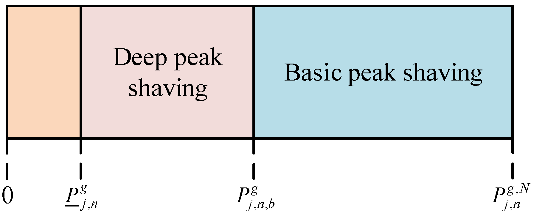
4. Analysis of Deep Peaking of Gas Turbines

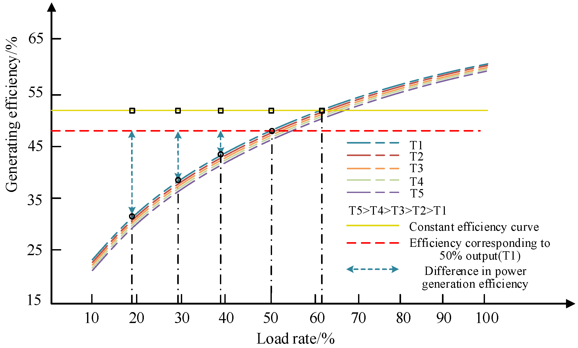
4.1. Load-Efficiency Characteristics of Gas Turbines at Variable Temperatures

This paper analyzes the relationship between the power generation efficiency of gas turbines and the ambient temperature and load factor, constructs the load-efficiency characteristic relationship of gas power generation under variable temperature, and calculates the deep-peaking energy loss cost of gas-generating units and the life loss cost of units.

Figure 1 shows the relationship of power generation efficiency of a typical F GTCC unit in a non-heating period with the load rate and temperature. T1–T5 indicate different ambient temperatures. In general, the efficiency difference due to different ambient temperatures during the low load rate phase can be neglected. The efficiency of GTCC units as a function of load rate and temperature can be expressed by the following equation:

$$\eta =\left\{\begin{array}{l}a\ln 100\phi +b\\ \phi \in [10,100]\end{array}\right.$$

(12)

where $\varphi$ is the GTCC unit load factor; and a and b are coefficients indicating the load factor-efficiency curves at different ambient temperatures.

4.2. Deep Peaking Cost Analysis

The participation of GTCC units in power system peaking can be divided into two modes: basic peak shaving and deep peak shaving, as shown in Figure 2. The reduction in power generation efficiency of GTCC units under low load rate operation causes part of the energy loss; at the same time, the deep-peaking operation of GTCC units will lead to a reduction in the unit’s service life and increase in the wear and tear costs. In order to accurately reflect the cost of deep-peaking operation, it is necessary to consider the energy loss and lifetime loss of GTCC units under deep peaking.

4.2.1. Cost of Lost Energy for Deep Peak Shaving of Units

The partial energy loss due to the reduced load factor during deep peak shaving of the GTCC unit, reduced gas initial temperature and compressor pressure ratio, and reduced generation efficiency can be expressed as follows:

$$C_{\mathrm{en}}={\displaystyle \frac{c({\eta }_{j,n,b}{P}_{j,n,t}^g-{\eta }_{j,n,t}{P}_{j,n,t}^g)}{P_{j,n,b}^g-P_{j,n,t}^g}}$$

(13)

where $c$ is the GTCC deep-peaking energy loss cost factor; ${\eta }_{j,n,b}$ and ${\eta }_{j,n,t}$ are the corresponding efficiencies with the basic peaking minimum output and deep peaking for unit n of gas-fired power station j, respectively; and $P_{j,n,t}^g$ and $P_{j,n,b}^g$ are the t-time output and the basic-peaking minimum output of unit n of gas-fired power station j, respectively.

4.2.2. Unit Life Wear and Tear Cost

In the deep-peaking operation mode, GTCC units are subjected to strain forces, high temperatures, and continuous loading forces, and the turbine rotor will produce certain losses due to low circumferential fatigue and creep, which shortens the unit life [27]. The rotor’s fracture perihelion N can be expressed by the Langer equation:

$$N={\left({\displaystyle \frac{R\ln 1/(1-\theta )}{4({\sigma }_a-{\sigma }_b)}}\right)}^2$$

(14)

In the formula, $R$ is the modulus of elasticity of a material; $\theta$ is the material section shrinkage factor; ${\sigma }_b$ is the limit value of the fatigue degree of the material; and ${\sigma }_a$ is the stress at the point of calculation. The calculation method is as follows: the receiving end load prediction error is used as a fuzzy parameter to portray the uncertainty of the receiving end load, as shown in the following equation:

$${\sigma }_a={\displaystyle \frac{Rm\mathrm{\Phi }{\alpha }^2}{8(1-\gamma )\varpi }}$$

(15)

In the formula, m is the coefficient of expansion of the rotor material; $\gamma$ is Poisson’s ratio; $\mathrm{\Phi }$ is the temperature rise rate; $\alpha$ is the thickness of the metal at the radius of the rotor; and $\varpi$ is the coefficient of thermal conductivity of the material.

The life loss rate $d$ due to the participation of GTCC units in deep peaking is as follows:

$$d={\displaystyle \frac{1}{N}}$$

(16)

The life loss rate caused by a unit with a capacity of 200 MW is 0.0006% per participation in deep variable load regulation [28]. The average cost of deep-peaking life loss for different classes of GTCC units can be estimated by the above method, as shown in the following equation:

$$C_{\mathrm{loss}}={\displaystyle \frac{{\displaystyle \sum _{e\in E}{C}_{e,\mathrm{unit}}}}{E\cdot N}}$$

(17)

In the formula, $C_{e,\mathrm{unit}}$ is the price of a GTCC unit with an e rating; and $E$ is the total number of types of units.

5. Gas–Hydro Coordinated Peaking Model Considering Source-Load Uncertainty and Deep Peaking

This section, based on the modeling of the hydroelectric power output and gas-fired power generation output, establishes the gas–hydro coordinated peak-shaving model, considering the source and load uncertainty of the system and the deep peak regulation of the gas-electric unit, and addresses the nonlinear part of the model by linearization methods.

5.1. Model Building

To establish the gas–hydro coordinated peak-shaving model considering source-load uncertainty and deep peaking, this section first establishes the hydroelectric power output model and gas-fired power generation output model, and then analyzes the system operation risk caused by source-load uncertainty. Finally, this section proposes the gas–hydro coordinated peaking model, which considers source-load uncertainty and deep peaking with the goal of maximizing the net profit of peak shaving.

5.1.1. Hydroelectric Power Output Modeling

The hydroelectric power plant output is determined by the head and the flow rate of the generating water, as shown in the following equation:

$$P_{i,m,t}^h=f_{i,m}^{phq}(H_{i,m,t},A_{i,m,t})$$

(18)

In the formula, $f_{i,m}^{phq}(•)$ is the power characteristic curve of unit m of hydropower station i. For hydropower stations with large reservoirs that have more than a daily regulation capacity, the head of the reservoir does not change significantly during the scheduling period, the effect of the head change on the power generation is generally not taken into account, and the unit output is in a two-dimensional nonlinear relationship with the flow rate. For the hydropower station with only a daily regulation capability, the head changes significantly during system peak shifting, leading to a three-dimensional nonlinear relationship between the hydropower station output, the head, and the flow rate. To reach a solution, this paper linearizes these relationships in the following sections.

5.1.2. Gas-Fired Power Generation Output Modeling

The generation output and gas consumption of a gas-fired generating set can be expressed by the following equation after considering the change in efficiency:

$$P_{j,n,t}^g=G_{j,n,t}\cdot LHV\cdot {\eta }_{j,n,t}^g$$

(19)

In the formula, $G_{j,n,t}$ is the gas consumption corresponding to the output of unit n of gas-fired power station j at time t $P_{j,n,t}^g$; $LHV$ is the low calorific value of natural gas; and ${\eta }_{j,n,t}^g$ is the generation efficiency of unit n of gas-fired power station j at time t.

5.1.3. Objective Function

$$\max I=I_1-I_2-I_3-I_4-I_5$$

(20)

The formula can be used to calculate the operating profit of gas–hydro coordinated peaking; $I_1$ is the operating revenue of gas–hydro coordinated power generation; $I_2$ is the operating cost of gas–hydro coordinated peaking; $I_3$ is the deep peaking losses for gas turbines; $I_4$ is the system standby cost; and $I_5$ is the cost of load shedding and water abandonment risk. The formula for calculating each benefit and cost is as follows:

(1)

Operational benefits of coordinated gas–hydro power generation

$$I_1={\displaystyle \sum _{t=1}^T({\displaystyle \sum _{i=1}^{N_I}{\displaystyle \sum _{m=1}^{N{H}_m}{C}_h\cdot P_{i,m,t}^h}+{\displaystyle \sum _{j=1}^{N_J}{\displaystyle \sum _{n=1}^{N{G}_n}{C}_g\cdot P_{j,n,t}^g)\cdot \mathrm{\Delta }t}}}}$$

(21)

In the formula, $N_I$ is the total number of hydroelectric power stations; $C_h$ is the feed-in tariff for hydropower; $P_{i,m,t}^h$ is the output of unit m of hydropower plant i at time t; $T$ is the scheduling run cycle; $N_J$ is the total number of gas-fired power stations; $C_g$ is the feed-in tariff for gas electricity; and $P_{j,n,t}^g$ is the output of unit n of gas-fired power station j at time t.

(2)

Operating costs of gas–hydro coordinated power generation

$$\begin{array}{ll}{I}_2=& {\displaystyle \sum _{t=1}^{\mathrm{T}}({\displaystyle \sum _{i=1}^{N_I}{\displaystyle \sum _{m=1}^{N{H}_m}{P}_{i,m,t}^h}\cdot C_{i,m,t}^h\cdot \mathrm{\Delta }t}}+{\displaystyle \sum _{j=1}^{N_J}{\displaystyle \sum _{n=1}^{N{G}_n}[K\cdot \frac{P_{j,n,t}^g}{{\eta }_{j,n}^g\cdot LHV}\cdot }}\mathrm{\Delta }t\\ & +z_{j,n,t}\cdot (1-z_{j,n,t-1})\cdot v_{j,n}])\end{array}$$

(22)

In the formula, $C_{i,m,t}^h$ is the unit price of electricity generated by unit m of hydropower plant i; $K$ is the price of natural gas; $z_{j,n,t}$ is the start–stop state 0–1 variable of unit n of gas-fired power station j in time period t (if it is 1, it means on; otherwise, it means off); and ${\nu }_{j,n}$ is the start-up cost of unit n of gas-fired power station j.

(3)

Deep peaking losses for gas turbines

$$I_3=\left\{\begin{array}{l}{\displaystyle \sum _{t=1}^{\mathrm{T}}{\displaystyle \sum _{j=1}^{N_J}{\displaystyle \sum _{n=1}^{N{G}_n}k(P_{j,n,k}^g-P_{j,n,t}^g)}}}\hfill \\ k=0,P_{j,n,k}^g={\overline{P}}_{j,n}^g,if(P_{j,n,b}^g\le P_{j,n,t}^g\le {\overline{P}}_{j,n}^g)\hfill \\ k=C_{loss}+C_{en},P_{j,n,k}^g=P_{j,n,b}^g,if({\underset{¯}{P}}_{j,n}^g\le P_{j,n,t}^g\le P_{j,n,b}^g)\hfill \end{array}\right.$$

(23)

In the formula, $P_{j,n,b}^g$ is the basic peaking minimum technical output of unit n of gas-fired power station j; and $k$ is the unit’s peaking cost variable, where a value of 0 indicates that the unit does not participate in peaking.

(4)

System Standby Costs

$$I_4={\displaystyle \sum _{t=1}^{\mathrm{T}}{\displaystyle \sum _{j=1}^{N_J}{\displaystyle \sum _{n=1}^{N{G}_n}(C_{j,n}^{up}{R}_{j,n,t}^{up}}+C_{j,n}^{dw}{R}_{j,n,t}^{dw})}}$$

(24)

In the formula, $C_{j,n}^{up}$ and $C_{j,n}^{dw}$ are the prices for the upper and lower standby capacities provided by GTCC unit n, respectively; and $R_{j,n,t}^{up}$ and $R_{j,n,t}^{dw}$ are the upper and lower standby capacities provided by GTCC unit n, respectively. Since hydropower basically operates at full capacity during the wet season, and it is difficult to provide sufficient standby capacity during the dry season due to the influence of incoming water, this paper only considers GTCC units with superior peak-regulating performance levels as the providers of system standby capacity.

(5)

Cost of Load Shedding and Abandonment Risks

$$I_5=C_{\mathrm{CVaR},\mathrm{L}}^{\mathrm{net}}$$

(25)

5.1.4. Restrictive Condition

(1)

System power balance constraints

$${\displaystyle \sum _{i=1}^{N_I}{\displaystyle \sum _{m=1}^{N{H}_m}{P}_{i,m,t}^h+{\displaystyle \sum _{j=1}^{N_J}{\displaystyle \sum _{n=1}^{N{G}_n}{P}_{j,m,t}^g}}}}=P{L}_{f,t}^{net}$$

(26)

(2)

Inter-reservoir hydraulic linkages

$$A_{i,t}^{in}=A_{i-1,t-\tau }+S_{i-1,t-\tau }+{\delta }_{i,t}$$

(27)

In the formula, $A_{i,t}^{in}$ is the incoming flow of hydropower plant i in time period t, m³/s; $A_{i-1,t-\tau }$ is hydroelectric power plant i − 1 in $t-\tau$ flow of electricity generation during the time period, m³/s; $S_{i-1,t-\tau }$ is the i − 1st hydropower plant in $t-\tau$ water discarded during the time period, m³/s; $\tau$ is the water flow lag time h between hydroelectric plant i − 1 and hydroelectric plant i; and ${\delta }_{i,t}$ is the interval flow between hydroelectric plant i − 1 and hydroelectric plant i at time t, m³/s.

(3)

Water balance constraints

$$V_{i,t}=V_{i,t-1}+3600\mathrm{\Delta }t(A_{i,t}^{in}-A_{i,t}-S_{i,t})$$

(28)

In the formula, $V_{i,t}$ is the reservoir capacity of hydropower plant i at the end of time period t, m³; $Q_{i,t}$ is the generation flow of hydropower plant i in time period t; and $S_{i,t}$ is the abandoned water flow rate of hydropower plant i in time period t, m³/s.

(4)

Reservoir capacity constraints

$${\underset{¯}{V}}_i\le V_{i,t}\le {\overline{V}}_i$$

(29)

In the formula, ${\underset{¯}{V}}_i$ and ${\overline{V}}_i$ are the lower and upper limits of the reservoir capacity of hydropower plant i in time period t, respectively; and $V_{i,t}$ is the reservoir capacity of hydropower plant i in time period t, m³.

(5)

Reservoir opening and closing capacity constraints

$$V_{i,0}=V_{i,begin}$$

(30)

$$V_{i,T}=V_{i,end}$$

(31)

In the formula, $V_{i,0}$ and $V_{i,T}$ are the reservoir capacities of hydropower plant i at the beginning and end of the scheduling period, respectively; and $V_{i,begin}$ and $V_{i,end}$ are the initial and final reservoir capacities of the hydropower plant, respectively.

(6)

Hydroelectric power plant outflow constraints

$${\underset{¯}{A}}_{i,t}\le A_{i,t}+S_{i,t}\le {\overline{A}}_{i,t}$$

(32)

where ${\underset{¯}{A}}_{i,t}$ and ${\overline{A}}_{i,t}$ are the lower and upper limits of the outflow flow of hydropower station i during time period t, respectively, m³/s.

(7)

Power plant unit output constraints

$$\left\{\begin{array}{l}{z}_{i,m,t}\cdot {\underset{¯}{P}}_{i,m}^h\le P_{i,m,t}^h\le z_{i,m,t}\cdot {\overline{P}}_{i,m}^h\hfill \\ z_{i,m,t}\in \left\{0,1\right\}\hfill \end{array}\right.$$

(33)

In the formula, ${\underset{¯}{P}}_{i,m}^h$ and ${\overline{P}}_{i,m}^h$ are the lower and upper limits of the output of unit m of hydropower station i, respectively; and $z_{i,m,t}$ is the operating state variable of unit m of hydropower plant i in time period t. If the unit is in operation, then $z_{i,m,t}=1$; if it is in its shutdown state, it is 0.

(8)

Hydroelectric power plant unit generation flow constraints

$$\left\{\begin{array}{l}{A}_{i,m}\le A_{i,m,t}\le {\overline{A}}_{i,m}\\ {\displaystyle \sum _{m=1}^{NHm}{A}_{i,m,t}=A_{i,t}}\end{array}\right.$$

(34)

In the formula, ${\underset{¯}{A}}_{i,m}$ and ${\overline{A}}_{i,m}$ are the lower and upper limits of the generation flow of unit m of hydropower plant i, respectively.

(9)

Hydroelectric power plant unit climbing rate constraints

$$-\mathrm{\Delta }{\overline{P}}_{i,m}^h\mathrm{\Delta }t\le P_{i,m,t+1}^h-P_{i,m,t}^h\le \mathrm{\Delta }{\overline{P}}_{i,m}^h\mathrm{\Delta }t$$

(35)

In the formula, $\mathrm{\Delta }{\overline{P}}_{i,m}^h$ is the rate of climb constraint for unit m of hydropower plant i, MW/h.

(10)

Hydroelectric power plant unit start-up and shutdown duration constraints

$$\left\{\begin{array}{l}{\displaystyle \sum _{d=t}^{\min (\mathrm{T},t+T{S}_{i,m}^h-1)}{z}_{i,m,d}\ge T{S}_{i,m}^h\cdot (z_{i,m,t}-z_{i,m,t-1})}\hfill \\ {\displaystyle \sum _{d=t}^{\min (\mathrm{T},t+T{C}_{i,m}^h-1)}(1-z_{i,m,d})\ge T{C}_{i,m}^h\cdot (z_{i,m,t-1}-z_{i,m,t})}\hfill \\ z_{i,m,t}\in \left\{0,1\right\}\hfill \end{array}\right.$$

(36)

In the formula, $T{S}_{i,m}^h$ and $T{C}_{i,m}^h$ are the minimum start and stop times for unit m of hydropower plant i, respectively.

(11)

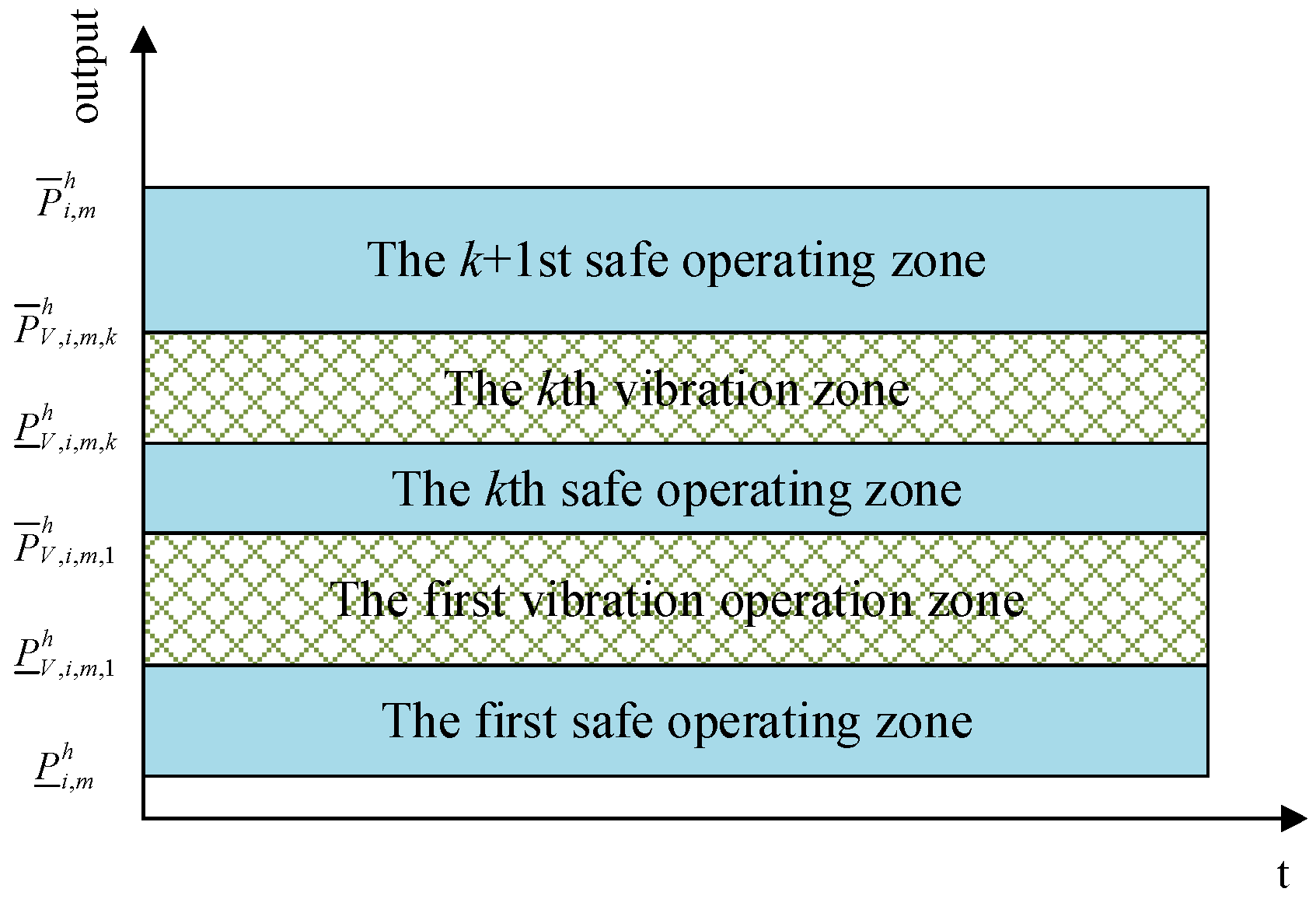
Hydroelectric power plant unit vibration zone constraints

$$(P_{i,m,t}^h-{\overline{P}}_{V,i,m,k}^h)(P_{i,m,t}^h-{\underset{¯}{P}}_{V,i,m,k}^h)\ge 0$$

(37)

In the formula, ${\overline{P}}_{V,i,m,k}^h$ and ${\underset{¯}{P}}_{V,i,m,k}^h$ are the upper and lower limits of the output of unit m of hydropower plant i in the kth vibration zone, respectively.

(12)

GTCC unit output constraints

$$\left\{\begin{array}{l}\begin{array}{l}{P}_{j,n,t}^g+R_{j,n,t}^{up}\le u_{j,n,t}\cdot {\overline{P}}_{j,n}^g\\ P_{j,n,t}^g-R_{j,n,t}^{dw}\ge u_{j,n,t}\cdot {\underset{¯}{P}}_{j,n}^g\end{array}\hfill \\ z_{j,n,t}\in \left\{0,1\right\}\hfill \end{array}\right.$$

(38)

In the formula, ${\underset{¯}{P}}_{j,n}^g$ and ${\overline{P}}_{j,n}^g$ are the lower and upper limits of unit output for gas-fired power plant j, respectively; the minimum steady-state output for GTCC units is 30% of the rated output; and $z_{j,n,t}$ is the operating state variable of unit n of gas-fired power station j in time period t (if unit n is in operation, then $z_{j,n,t}=1$; if it is in the shutdown state, it is ${\mathrm{z}}_{j,n,t}=0$).

(13)

GTCC unit climbing rate constraints

$$(P_{j,n,t}^g+R_{j,n,t}^{up})-(P_{j,n,t-1}^g-R_{j,n,t-1}^{dw})\le \mathrm{\Delta }{\overline{P}}_{j,n}^g\mathrm{\Delta }t(1-e_{j,n,t})+{\underset{¯}{P}}_{j,n}^g{e}_{j,n,t}$$

(39)

$$(P_{j,n,t-1}^g+R_{j,n,t-1}^{up})-(P_{j,n,t}^g-R_{j,n,t}^{dw})\le \mathrm{\Delta }{\underset{¯}{P}}_{j,n}^g\mathrm{\Delta }t(1-q_{j,n,t})+{\underset{¯}{P}}_{j,n}^g{q}_{j,n,t}$$

(40)

$$e_{j,n,t}-q_{j,n,t}=z_{j,n,t}-z_{j,n,t-1}$$

(41)

$$e_{j,n,t}+q_{j,n,t}\le 1$$

(42)

In the formula, $\mathrm{\Delta }{\overline{P}}_{j,n}^g$ and $\mathrm{\Delta }{\overline{P}}_{j,n}^g$ are the upward and downward climb rates, MW/h, respectively, for unit n of gas-fired power plant j; and $e_{j,n,t}$ and $q_{j,n,t}$ are the auxiliary variables for the start and stop of unit n of gas-fired power station j at time t, respectively.

(14)

System standby capacity constraints

$${\displaystyle \sum _{j=1}^{N_J}{\displaystyle \sum _{n=1}^{N{G}_n}{R}_{j,n,t}^{\mathrm{up}}\ge {\xi }_{L,t}^{net,u}}}$$

(43)

$${\displaystyle \sum _{j=1}^{N_J}{\displaystyle \sum _{n=1}^{N{G}_n}{R}_{j,n,t}^{\mathrm{dw}}\ge -{\xi }_{L,t}^{net,l}}}$$

(44)

$$0\le R_{j,n,t}^{\mathrm{up}}\le \mathrm{\Delta }{\overline{P}}_{j,n}^g\mathrm{\Delta }t$$

(45)

$$0\le R_{j,n,t}^{\mathrm{dw}}\le \mathrm{\Delta }{\underset{¯}{P}}_{j,n}^g\mathrm{\Delta }t$$

(46)

The system power balance is ensured in any case within the net load tolerance error interval by arranging the standby capacity to cope with the uncertainty of the net load. Since the amount of net load fluctuation is balanced by Equation (1), the effect of net load fluctuation can be disregarded in the system power balance constraint.

(15)

Transmission corridor capacity constraints

$${\underset{¯}{S}}_{l,t}\le {\displaystyle \sum _{i=1}^{NI}{\displaystyle \sum _{m=1}^{NHm}{P}_{i,m,t}^h}}+{\displaystyle \sum _{j=1}^{NJ}{\displaystyle \sum _{n=1}^{NGj}{P}_{j,n,t}^g}}\le {\overline{S}}_{l,t}$$

(47)

In the formula, ${\underset{¯}{S}}_{l,t}$ and ${\overline{S}}_{l,t}$ are the lower and upper limits of the transmission channel capacity, respectively.

5.2. Model Solution

The model constructed in Section 3.1 is essentially a MINLP model, where the nonlinear factors in the model are linearized and thus transformed into a MILP model to improve the efficiency of the solution.

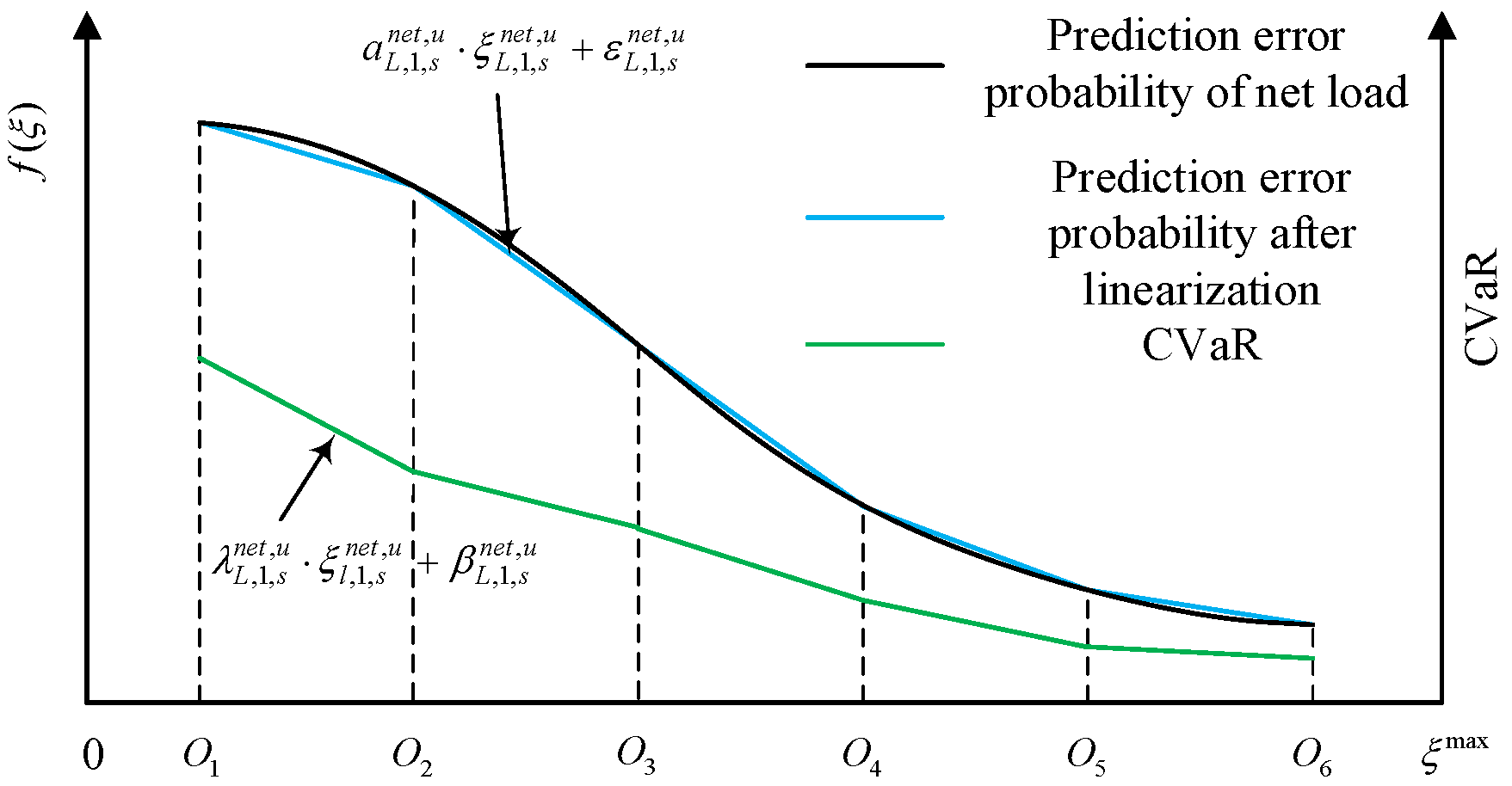
5.2.1. CVaR Segment Linearization

In the equation for $C_{\mathrm{CVaR},\mathrm{L}}^{\mathrm{net}}$, due to the increased computational complexity and time required for complex nonlinear and nonconvex functions, the solution difficulty is relatively high. Therefore, this paper is based on the piecewise linear approximation method. We linearize the integral term in the equation. The integral terms in the equation are, respectively,$E_{\mathrm{L},t}^{\mathrm{net},u}$ and $E_{\mathrm{L},t}^{\mathrm{net},l}$. The linearization method is shown in Figure 3.

The specific methods are as follows:

$$\begin{array}{l}{E}_{\mathrm{L},t}^{\mathrm{net},u}({\xi }_{\mathrm{L},t}^{\mathrm{net},u})={\displaystyle {\int }_{{\xi }_{\mathrm{L},t}^{\mathrm{net},u}}^{{\xi }_{\mathrm{L},t}^{\mathrm{net},\max }}(x}-{\xi }_{\mathrm{L},t}^{\mathrm{net},u})f(x)dx\\ ={\displaystyle \sum _{s=1}^{n_s}({\lambda }_{\mathrm{L},t,s}^{\mathrm{net},u}{\xi }_{\mathrm{L},t,s}^{\mathrm{net},u}+{\beta }_{\mathrm{L},t,s}^{\mathrm{net},u}{\rho }_{\mathrm{L},t,s}^{\mathrm{net},u})}\end{array}$$

(48)

$${\displaystyle \sum _{s=1}^{n_s}{\xi }_{\mathrm{L},t,s}^{\mathrm{net},u}=}{\xi }_{\mathrm{L},t}^{\mathrm{net},u}$$

(49)

$${\displaystyle \sum _{s=1}^{n_s}{\rho }_{\mathrm{L},t,s}^{\mathrm{net},u}=}1$$

(50)

$$O_{\mathrm{L},t,s}^{\mathrm{net},u}{\rho }_{\mathrm{L},t,s}^{\mathrm{net},u}\le {\xi }_{\mathrm{L},t,s}^{\mathrm{net},u}\le O_{\mathrm{L},t,s+1}^{\mathrm{net},u}{\rho }_{\mathrm{L},t,s}^{\mathrm{net},u}$$

(51)

In the formula, $n_s$ is the total number of subparagraphs; ${\xi }_{\mathrm{L},t,s}^{\mathrm{net},u}$ and ${\rho }_{\mathrm{L},t,s}^{\mathrm{net},u}$ are the values and 0–1 variables, respectively, for which the net load prediction error at time t is located in the s-th subsection; ${\lambda }_{\mathrm{L},t,s}^{\mathrm{net},u}$ and ${\beta }_{\mathrm{L},t,s}^{\mathrm{net},u}$ are the slope and intercept of the s-th segment of the prediction error of the net load at time t, respectively; and $O_{\mathrm{L},t,s}^{\mathrm{net},u}$ is the s-th segmentation point of the net load forecast error in time period t.

The same linearization process is applied to another integral term, and the final result is as follows:

$$\begin{array}{c}{C}_{\mathrm{CVaR},\mathrm{L}}^{\mathrm{net}}={\displaystyle \sum _{t=1}^{\mathrm{T}}{\epsilon }^u[{\displaystyle \sum _{s=1}^{n_s}({\lambda }_{\mathrm{L},t,s}^{\mathrm{net},u}{\xi }_{\mathrm{L},t,s}^{\mathrm{net},u}+{\beta }_{\mathrm{L},t,s}^{\mathrm{net},u}{\rho }_{\mathrm{L},t,s}^{\mathrm{net},u})}}+\\ {\epsilon }^{\mathrm{l}}{\displaystyle \sum _{s=1}^{n_s}({\lambda }_{\mathrm{L},t,s}^{\mathrm{net},l}{\xi }_{\mathrm{L},t,s}^{\mathrm{net},l}+{\beta }_{\mathrm{L},t,s}^{\mathrm{net},l}{\rho }_{\mathrm{L},t,s}^{\mathrm{net},l})}]\end{array}$$

(52)

5.2.2. Linearization of Hydroelectric Output Characteristics

(1)

Linearization of the head of a daily regulated hydroelectric power station

We set the head interval of a hydropower plant i with daily regulation performance as $\left[{\underset{¯}{H}}_{i,m},{\overline{H}}_{i,m}\right]$. This is divided into three subintervals, as shown in Figure 4. The generating head of hydro unit m in time period t must be located in one of the subintervals:

$${\displaystyle \sum _{l=1}^3{\partial }_{i,m,t}^l{H}_{i,m}^{l-1}\le H_{i,m,t}\le {\displaystyle \sum _{l=1}^3{\partial }_{i,m,t}^l{H}_{i,m}^l}}$$

(53)

$${\displaystyle \sum _{l=1}^3{\partial }_{i,m,t}^l=1},{\partial }_{i,m,t}^l\in [0,1]$$

(54)

$$H_{i,m}^0={\underset{¯}{H}}_{i,m}$$

(55)

$$H_{i,m}^3={\overline{H}}_{i,m}$$

(56)

In the formula, ${\partial }_{i,m,t}^l$ is the head discrete interval 0–1 variable, and a value of 1 indicates that the head of unit m of hydropower plant i is located in the l-th interval.

A set of characteristic curves is selected as the unit power characteristic curves in each subinterval, the head will take a fixed value, and the unit output will only be related to the generation flow. Among the three subintervals, curves 1, 2, and 3 are selected as representatives of each subinterval.

Thus, the correlation between the unit output characteristic curve and the head can be expressed as follows:

$$-{\overline{P}}_{i,m}^h(1-{\partial }_{i,m,t}^1)\le P_{i,m,t}^h-f_{i,m}^1(A_{i,m,t})\le {\overline{P}}_{i,m}^h(1-{\partial }_{i,m,t}^1)$$

(57)

$$-{\overline{P}}_{i,m}^h(1-{\partial }_{i,m,t}^2)\le P_{i,m,t}^h-f_{i,m}^2(A_{i,m,t})\le {\overline{P}}_{i,m}^h(1-{\partial }_{i,m,t}^2)$$

(58)

$$-{\overline{P}}_{i,m}^h(1-{\partial }_{i,m,t}^3)\le P_{i,m,t}^h-f_{i,m}^3(A_{i,m,t})\le {\overline{P}}_{i,m}^h(1-{\partial }_{i,m,t}^3)$$

(59)

In the formula, $f_{i,m}^l(A_{i,m,t})$ is the characteristic function of unit m output and generation flow of hydropower plant i in the 1st sub-interval, which can be considered a two-dimensional relationship between output and generation flow at the representative head of the respective interval. The unified constraint on the relaxation and the specific curve is determined by the above-mentioned equations, for which the specific procedure can be found in the literature [29].

(2)

Linearization of unit power characteristic curve

For the power characteristic function of unit m of hydropower unit i at a specific head, the generation flow of unit m of hydropower plant i is discretized into V intervals.

$$\left\{\begin{array}{l}{\underset{¯}{A}}_{i,m}=A_{i,m}^0<A_{i,m}^1<\cdots <A_{i,m}^v<A_{i,m}^V\hfill \\ P_{i,m}^{h,v}=f(A_{i,m}^v)\hfill \\ n_{i,m,t}^v{A}_{i,m}^{v-1}\le A_{i,m,t}^v\le n_{i,m,t}^v{A}_{i,m}^v\hfill \\ {\displaystyle \sum _{v=1}^V{A}_{i,m,t}^v=A_{i,m,t}}\hfill \\ {\displaystyle \sum _{v=1}^V{n}_{i,m,t}^v=1}\hfill \end{array}\right.$$

(60)

In the formula, $A_{i,m}^v$ and $P_{i,m}^{h,v}$ are the generation flow and its corresponding output at the vth interpolation point, respectively; $A_{i,m,t}^v$ is the value of the generation flow of unit m of hydropower plant i in the vth flow interval of time period t; and $n_{i,m,t}^v$ is 0–1 variables. When ${\displaystyle \sum _{v=1}^V{n}_{i,m,t}^v=1}$, it is guaranteed that the generation flow of unit m of hydropower plant i in time period t is located in a unique partition. Therefore, the hydroelectric unit output can be expressed as follows:

$$P_{i,m}^h={\displaystyle \sum _{v=1}^V[n_{i,m,t}^v{A}_{i,m}^{v-1}+\frac{P_{i,m}^{h,v}-P_{i,m}^{h,v-1}}{A_{i,m}^v-A_{i,m}^{v-1}}(A_{i,m,t}^v-n_{i,m,t}^v{A}_{i,m}^{v-1})]}$$

(61)

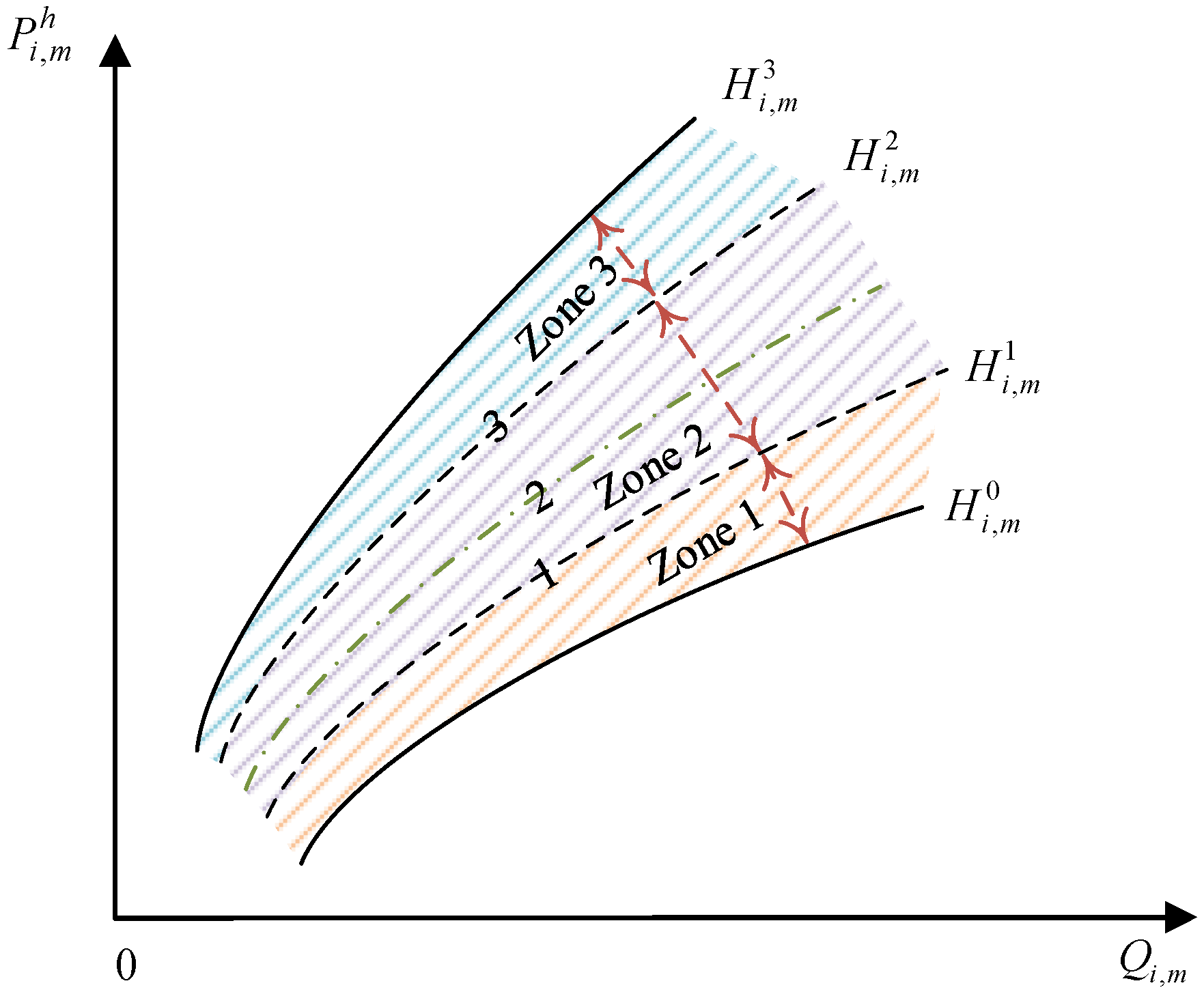
5.2.3. Constrained Linearization of Vibration Zones in Hydroelectric Units

The hydroelectric power plant unit vibration zone constraint condition equation is a nonlinear constraint, which can split the hydroelectric power unit output into discrete intervals, as shown in Figure 5.

The specific methods are as follows:

$${\displaystyle \sum _{k=1}^{K+1}{r}_{i,m,t}^k=z_{i,m,t}},r_{i,m,t}^k\in \left\{0,1\right\}$$

(62)

$${\displaystyle \sum _{k=1}^{K+1}{r}_{i,m,t}^k{\underset{¯}{P}}_{i,m,k}^h\le P_{i,m,t}^h\le {\displaystyle \sum _{k=1}^{K+1}{r}_{i,m,t}^k}{\overline{P}}_{i,m,k}^h}$$

(63)

In the formula, $r_{i,m,t}^k$ represents discretized auxiliary variables. When $r_{i,m,t}^k=1$, the unit m output of hydropower plant i is located in the safe operating zone k; and ${\underset{¯}{P}}_{i,m,k}^h$ and ${\overline{P}}_{i,m,k}^h$ denote the lower and upper limits of safety zone k for unit m output of hydropower plant i, respectively, which must satisfy the following constraints:

$${\underset{¯}{P}}_{i,m,1}^h={\underset{¯}{P}}_{i,m}^h{\overline{P}}_{V,i,m,k}^h={\underset{¯}{P}}_{i,m,k+1}^h$$

(64)

$${\overline{P}}_{i,m,k}^h={\underset{¯}{P}}_{V,i,m,k}^h$$

(65)

$${\overline{P}}_{i,m,k+1}^h={\overline{P}}_{i,m}^h$$

(66)

5.2.4. Linearization of the Objective Function

The start–stop cost model for GTCC units is nonlinear. In the following, by introducing the variable $y_{j,n,t}$, we linearize it:

$$\left\{\begin{array}{l}{y}_{j,n,t}\le l\cdot z_{j,n,t}\hfill \\ y_{j,n,t}\le z_{j,n,t-1}\hfill \\ y_{j,n,t}\ge z_{j,n,t-1}-l\cdot (1-z_{j,n,t})\hfill \\ y_{j,n,t}\in [0,l]\hfill \end{array}\right.$$

(67)

In the formula, l is the upper limit of $u_{j,n,t-1}$.

Through the above methodology, we used the MATLAB compilation environment combined with the YALMIP toolkit (developed by Johan Löfberg, Linköping University, Linköping, Sweden) to invoke the commercial solver IBM ILOG CPLEX (12.8.0.) in order to solve the model. The main computing environment was an Intel Core i5, octa-core CPU with 2.7 GHz and 16 GB of RAM.

6. Case Study

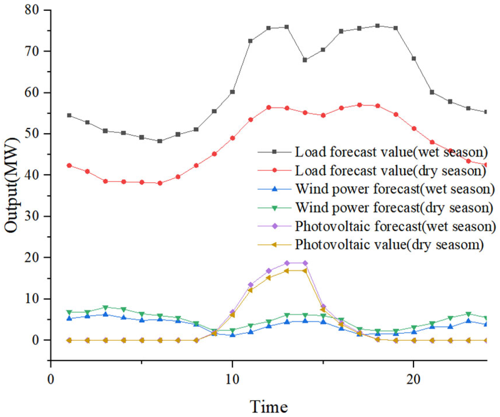
6.1. Basic Parameters

The calculation example in this paper includes four gas-fired generating units, four hydroelectric units, wind farms with a planned installed capacity of 11,500 kW, a photovoltaic installed capacity of 18,700 kW, and gas-fired generating units with a total installed capacity of 41,500 kW. We selected 27 August in the 2021 wet season and 20 December in the dry period as two typical cases of the wet season and dry periods, respectively. The risk cost coefficient of load cutting and the risk cost coefficient of water abandonment are 300 USD/MWh and 200 USD/MWh, respectively.

The forecast data for the load as well as wind and PV are shown in Figure 6.

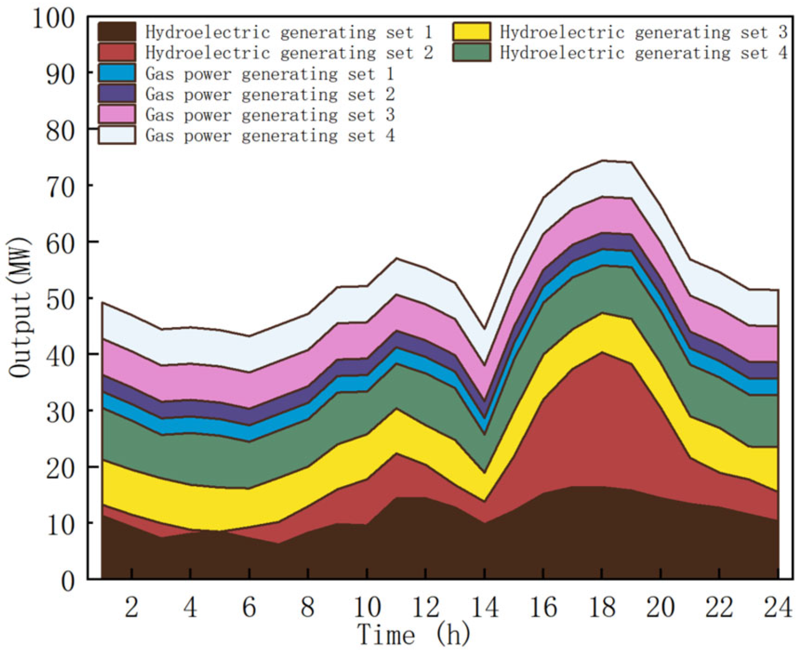
6.2. Analysis of Example Simulation Results

In order to verify the effectiveness of the peaking methods that take into account the system operation risk, the following four strategies were set up for comparison, respectively:

Case 1: The system operational risk and standby capacity of gas-fired generation are not taken into account;

Case 2: Taking into account the system operational risk;

Case 3: Taking into account the system operational risk and standby capacity of gas-fired generations;

Case 4: Considering 2% of the net load forecast as a static standby to address system operational risk, and considering 5% of the net load forecast as a static standby to address system operational risk.

The operating economic indicators under the four cases are shown in Figure 7.

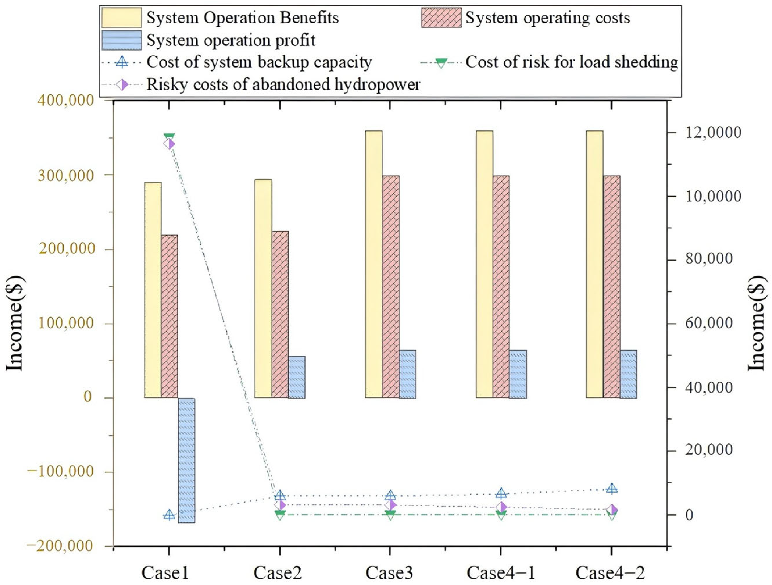
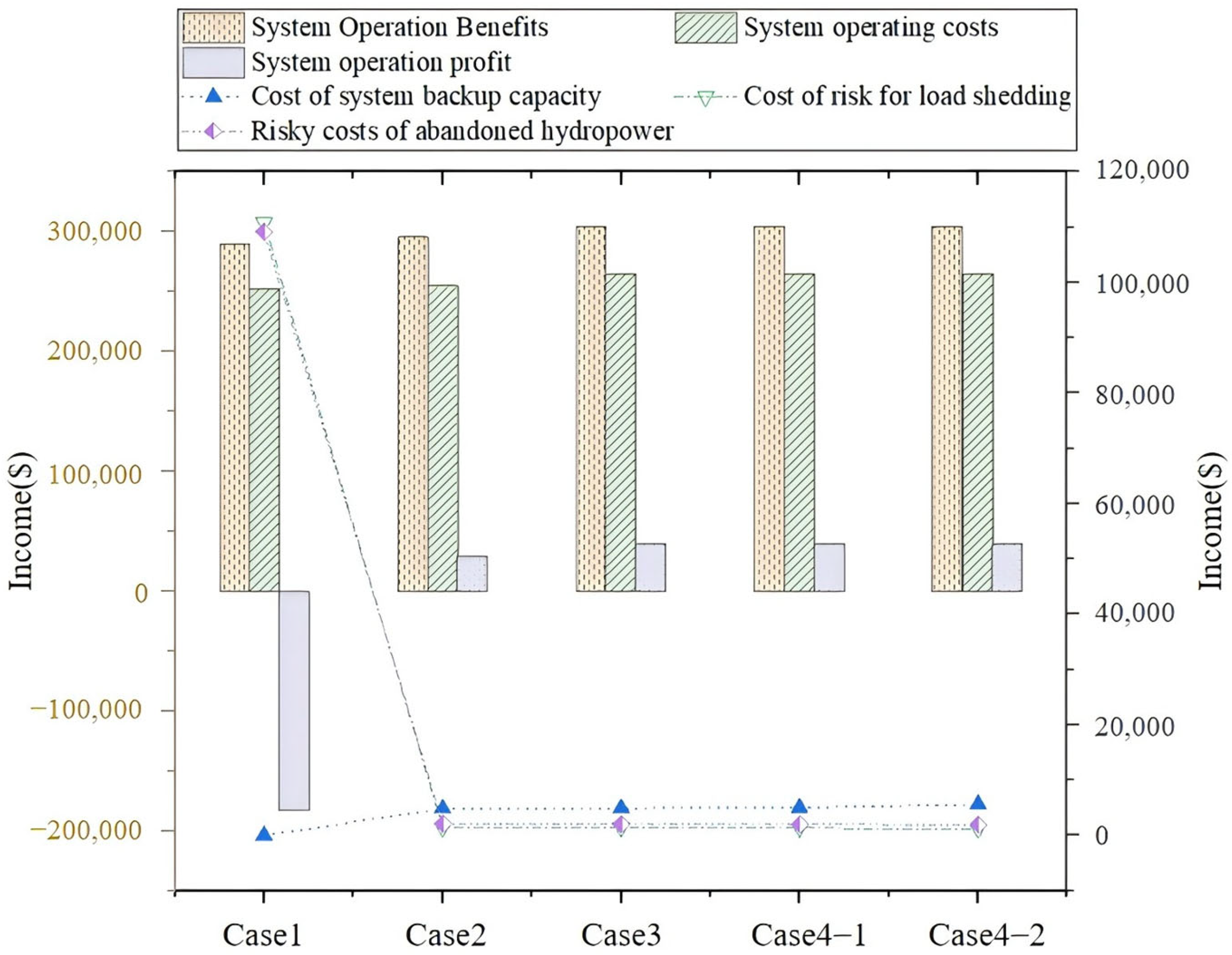
6.3. Analysis of the Results of the Calculation and System Operational Risk

The comparison of Case 1 and Case 2 in Figure 7 and Figure 8 shows that Case 1 has the lowest ability to cope with the system risk during the abundant and dry periods, and the system profits are −USD 167,500 and −USD 83,400 when the losses of the risks of load shedding and water abandonment are taken into account, respectively. Case 2 obtains profits of USD 56,800 and USD 29,800 during the abundant and dry periods, respectively. Case 3 optimizes the risks of load shedding and water abandonment through the provision of standby capacity by GTCC units, and the improvements in profit are about 12% and 36%, respectively, compared with Case 2.

When comparing Case 3 and 4 at the same time, taking the wet season as an example, the CVaR results of Cases 4–1 and 4–2 after considering the static standby are reduced by USD 640 and USD 1500, respectively, and the reserved standby costs are increased by USD 660 and USD 2200, respectively. In particular, the upper standby capacity of Case 4–2 is excessively large, meaning in the optimal solution tends to be conservative, and the overall profit of the system is reduced by USD 670. Therefore, although Case 4 can better weaken the risk of load cutting and water abandonment caused by source-load uncertainty, Case 3 takes into account the system economy and risk, and it achieves the purpose of dynamically and efficiently allocating the peaking resources, which provides certain ideas for the formulation of the peak-shaving scheme of the power system.

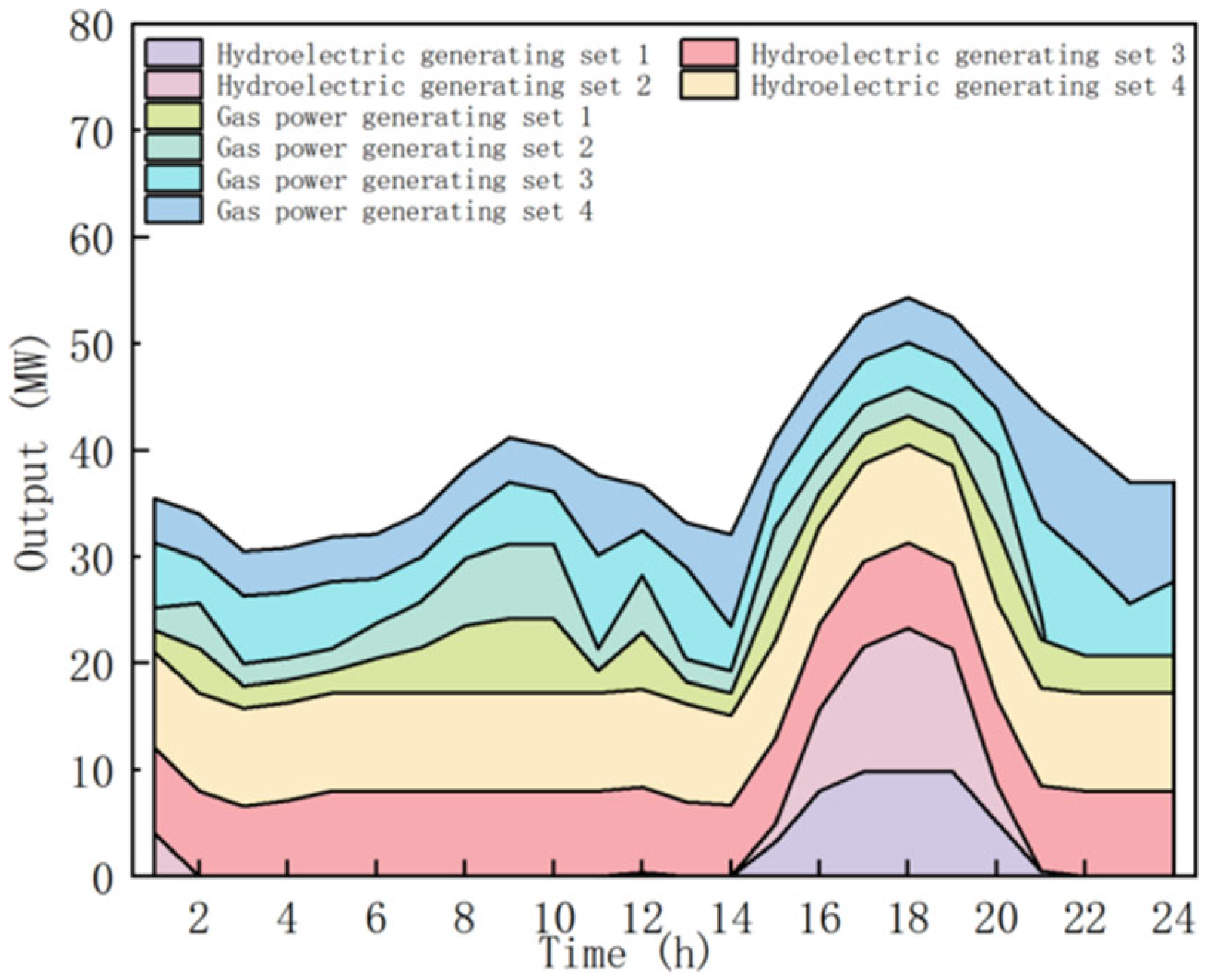
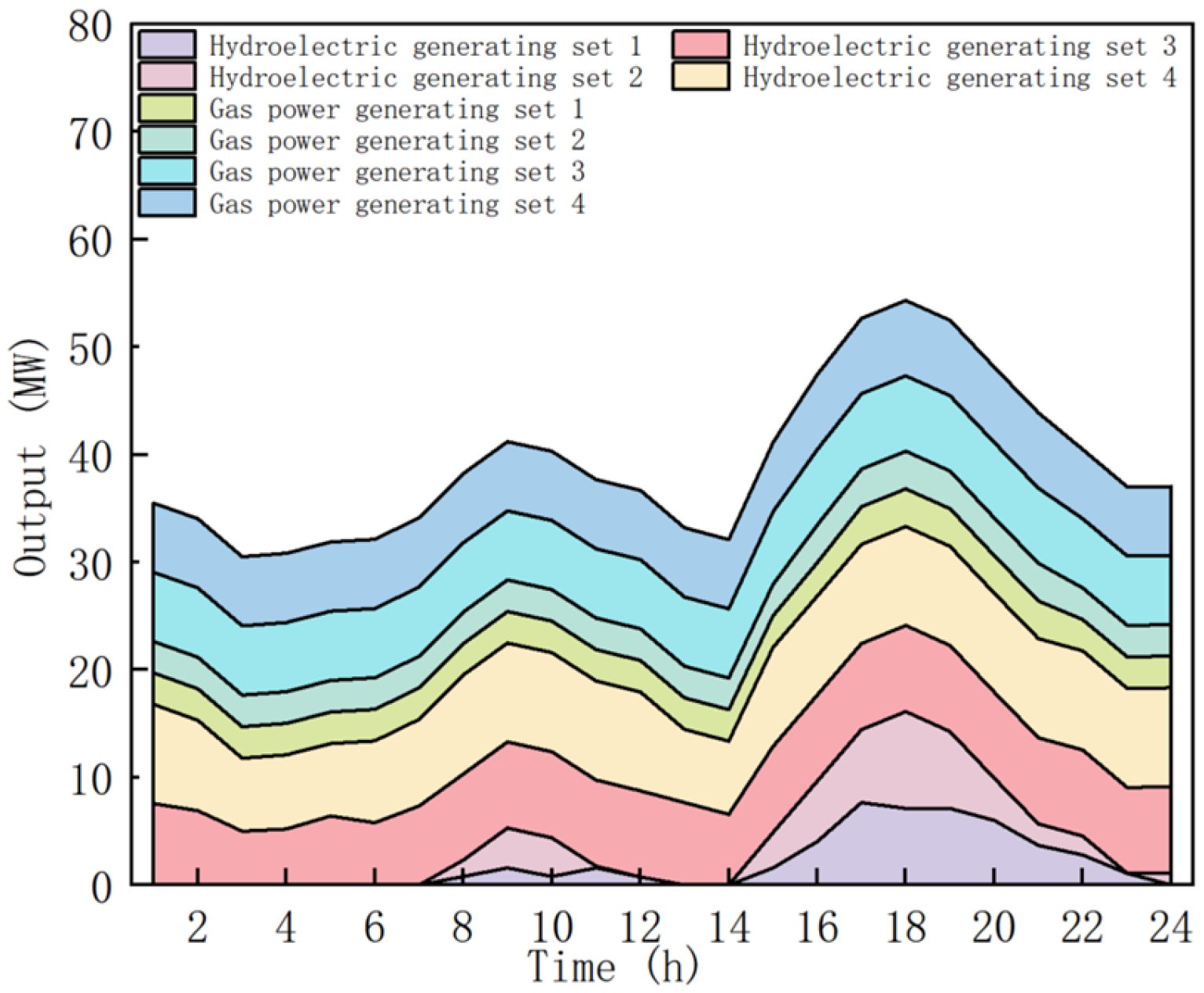
6.4. Analysis of the Results Considering Source-Load Uncertainty and Deep Peaking

• Analysis of the Results for Power Optimization

Figure 9, Figure 10, Figure 11 and Figure 12 present information on gas and hydroelectric power plant outputs under Cases 2 and 3 during periods of abundance and depletion.

As can be seen from Figure 9, Figure 10, Figure 11 and Figure 12, the output of the gas power station in Case 2 during the wet season fluctuates clearly, and the GTCC units start and stop more often, with the start and stop cost USD 1896 in the whole cycle; meanwhile, the output of the gas power station in Case 3 is more stable in the whole cycle, and the units in Case 3 have no downtime during the wet season. Moreover, the risk of load shedding is the same as that of water abandonment in the two cases. Case 3 improves the system profit by 14.45% after deep peak shaving.

For the dry season, the risk of system water abandonment increased by CNY 1040; in Case 3, the Hydro Unit 1 and Hydro Unit 2 stations increase their output during the net load peak period (Period 16–Period 21) to reduce the remaining load peak–valley difference. Simultaneously, the peaking compensation price is lowered during this period. Gas electric unit Nos. 2, 3, and 4 maintain the basic peaking minimum output, avoiding water abandonment loss of hydropower. Although the pollutant discharge management cost increases by USD 339, the system profit improves by 36.03%. Overall, the gas–hydropower plant responds to the net load-peaking demand by coordinating the output during the abundant period, fully leveraging the coupling characteristics of hydropower. Case 3 adopts the deep peak-regulation model to manage system operation risks, thereby enhancing system operational economy and flexibility while reducing operational risks. The power delivery method tracks load fluctuations at the receiving end, ensuring a more stable gas power unit output during the intra-day dispatch phase.

7. Conclusions

This paper first proposes a gas–hydro coordinated peak-shaving model. Then, it quantifies the operational risk caused by system source-load uncertainty using CVaR theory. Next, it proposes a strategy for gas-fired power generation deep peak shaving, and it establishes a gas–hydro coordinated peak-shaving model considering risk constraints and deep peak shaving. Finally, an optimization analysis is presented on the established gas–hydro coordinated peaking model with a specific arithmetic example, and the following conclusions can be drawn:

(1) In this paper, we propose a method to quantify the risk of system operation caused by source-load uncertainty using CVaR theory. We demonstrate that incorporating risk constraints can integrate the uncertainties on both the source and load sides of the system. By using gas turbines to provide spare capacity, we can reduce the operational risk associated with insufficient system peaking capacity. Additionally, setting appropriate risk cost coefficients allows us to balance the system's economy and robustness. (2) This paper considers the model of deep peak regulation to manage source-load uncertainty and reduce abandoned water. The proposed strategy for deep peak shifting of gas power generation can realize the smooth output of gas power, give full play to the coupling characteristics of hydropower, and reduce the amount of water discarded by hydropower during the wet season. At the same time, through the formulation of a reasonable, economic, robust scheduling plan, the optimal net load tolerance error interval can be obtained to achieve the effective consumption of wind power and reduce the risk of system load shedding. Compared to scheduling methods that only consider risk constraints, our approach increases total system profits by 12% and 36% during the wet and dry seasons, respectively, enhancing both the economy and flexibility of system operations. (3) The nonlinear factors in the model are addressed through linearization methods, effectively avoiding hydropower unit outputs falling into vibration zones. The number of segments in the PLA method is eight, and the model solution time is 759 s, which meets the timeliness requirements for day-ahead scheduling under complex constraints. This study mainly focuses on the coordinated operation mode of gas, electricity, and hydropower. Meanwhile, the role of other renewable energy sources (such as biomass energy, geothermal energy, etc.) in peak regulation is not fully considered. Future studies could explore how these renewable energy sources can be combined with gas–water coordinated peak-reduction strategies to build a more comprehensive and flexible energy management system. Additionally, although the conditional risk value theory is adopted to quantify the system operation risk caused by the source-load uncertainty, the design of the risk management strategy still needs to be further improved. Future work could focus on comparative studies of multiple risk assessment models and seek to optimize risk management strategies in different climate and market settings. In summary, further research in multi-energy complementarity and risk management could provide more comprehensive solutions for power system optimization in high-altitude environments.

References

1. Pingkuo, L.; Huan, P. What drives the green and low-carbon energy transition in China?: An empirical analysis based on a novel framework. Energy 2021, 239, 122450. [Google Scholar] [CrossRef]
2. Tian, C.; Huang, G.; Xie, Y. Systematic evaluation for hydropower exploitation rationality in hydro-dominant area: A case study of Sichuan Province, China. Renew. Energy 2020, 168, 1096–1111. [Google Scholar] [CrossRef]
3. Li, Y.; Zhao, K.; Zhang, F. Identification of key influencing factors to Chinese coal power enterprises transition in the context of carbon neutrality: A modified fuzzy DEMATEL approach. Energy 2022, 263, 125427. [Google Scholar] [CrossRef]
4. Ding, Y.; Hao, J.; Li, A.; Wang, X.; Zhang, X.; Liu, Y. Numerical Simulation of Combustion and Emission Characteristics during Gas Turbine Startup Procedure. Energies 2022, 15, 5444. [Google Scholar] [CrossRef]
5. Fan, G.; Lu, X.; Chen, K.; Zhang, Y.; Han, Z.; Yu, H.; Dai, Y. Comparative analysis on design and off-design performance of novel cascade CO2 combined cycles for gas turbine waste heat utilization. Energy 2022, 254, 124222. [Google Scholar] [CrossRef]
6. Wang, X.; Duan, L.; Zhu, Z. Peak regulation performance study of GTCC based CHP system with compressor inlet air heating method. Energy 2022, 262, 125366. [Google Scholar] [CrossRef]
7. Zheng, Z.; Zuo, Y.; Wen, H.; Zhang, J.; Zhou, G.; Xu, L.; Sun, H.; Yang, M.; Yan, K.; Zeng, J. Natural gas characteristics and gas-source comparisons of the lower triassic Jialingjiang formation, Eastern Sichuan basin. Geoenergy Sci. Eng. 2022, 221, 111165. [Google Scholar] [CrossRef]
8. Cheng, Q.; Luo, P.; Liu, P.; Li, X.; Ming, B.; Huang, K.; Xu, W.; Gong, Y. Stochastic short-term scheduling of a wind-solar-hydro complementary system considering both the day-ahead market bidding and bilateral contracts decomposition. Int. J. Electr. Power Energy Syst. 2022, 138, 107904. [Google Scholar] [CrossRef]
9. Huang, K.; Liu, P.; Ming, B.; Kim, J.-S.; Gong, Y. Economic operation of a wind-solar-hydro complementary system considering risks of output shortage, power curtailment and spilled water. Appl. Energy 2021, 290, 116805. [Google Scholar] [CrossRef]
10. Jin, X.; Liu, B.; Liao, S.; Cheng, C.; Yan, Z. A Wasserstein metric-based distributionally robust optimization approach for reliable-economic equilibrium operation of hydro-wind-solar energy systems. Renew. Energy 2022, 196, 204–219. [Google Scholar] [CrossRef]
11. Morillo, J.L.; Zephyr, L.; Pérez, J.F.; Cadena, A.; Anderson, C.L. Distribution-free chance-constrained load balance model for the operation planning of hydrothermal power systems coupled with multiple renewable energy sources. Int. J. Electr. Power Energy Syst. 2022, 142, 108319. [Google Scholar] [CrossRef]
12. Jiang, J.; Ming, B.; Liu, P.; Huang, Q.; Guo, Y.; Chang, J.; Zhang, W. Refining long-term operation of large hydro–photovoltaic–wind hybrid systems by nesting response functions. Renew. Energy 2023, 204, 359–371. [Google Scholar] [CrossRef]
13. Guo, Y.; Ming, B.; Huang, Q.; Wang, Y.; Zheng, X.; Zhang, W. Risk-averse day-ahead generation scheduling of hydro–wind–photovoltaic complementary systems considering the steady requirement of power delivery. Appl. Energy 2022, 309, 118467. [Google Scholar] [CrossRef]
14. Liao, S.; Liu, H.; Liu, B.; Zhao, H.; Wang, M. An information gap decision theory-based decision-making model for complementary operation of hydro-wind-solar system considering wind and solar output uncertainties. J. Clean. Prod. 2022, 348, 131382. [Google Scholar] [CrossRef]
15. Jin, X.; Liu, B.; Liao, S.; Cheng, C.; Zhang, Y.; Zhao, Z.; Lu, J. Wasserstein metric-based two-stage distributionally robust optimization model for optimal daily peak shaving dispatch of cascade hydroplants under renewable energy uncertainties. Energy 2022, 260, 125107. [Google Scholar] [CrossRef]
16. Behnamfar, M.R.; Barati, H.; Karami, M. Stochastic Multi-Objective Short-term Hydro-thermal Self-scheduling in Joint Energy and Reserve Markets Considering Wind-Photovoltaic Uncertainty and Small Hydro Units. J. Electr. Eng. Technol. 2021, 16, 1327–1347. [Google Scholar] [CrossRef]
17. Hong, Z.; Peihua, J.; Wei, P.; Peitong, H. Research on deep peaking costallocation mechanism considering peaking demand subject and thermal powerunit. Energy Rep. 2024, 12, 158–172. [Google Scholar] [CrossRef]
18. Wu, X.; Zhang, J.; Wei, X.; Cheng, C.; Cheng, R. Short-Term Hydro-Wind-PV peak shaving scheduling using approximate hydropower output characters. Renew. Energy 2024, 236, 121502. [Google Scholar] [CrossRef]
19. Zhang, J.; Guo, A.; Wang, Y.; Chang, J.; Wang, X.; Wang, Z.; Tian, Y.; Jing, Z.; Peng, Z. How to achieve optimal photovoltaic plant capacity in hydro-photovoltaic complementary systems: Fully coupling long-term and short-term operational modes of cascade hydropower plants. Energy 2024, 313, 134161. [Google Scholar] [CrossRef]
20. Wang, T.; Jiang, X.; Jin, Y.; Song, D.; Yang, M.; Zeng, Q. Peaking Compensation Mechanism for Thermal Units and Virtual Peaking Plants Union Promoting Curtailed Wind Power Integration. Energies 2019, 12, 3299. [Google Scholar] [CrossRef]
21. Nozarian, M.; Seifi, H.; Sheikh-El-Eslami, M.K.; Delkhosh, H. Hydro Thermal Unit Commitment involving Demand Response resources: A MILP formulation. Electr. Eng. 2022, 105, 175–192. [Google Scholar] [CrossRef]
22. Code for Design of Combined-Cycle Power Plant. 2020. Available online: https://d.wanfangdata.com.cn/standard/DL/T 5174-2020 (accessed on 23 October 2020).
23. Hou, J.; Yu, W.; Xu, Z.; Ge, Q.; Li, Z.; Meng, Y. Multi-time scale optimization scheduling of microgrid considering source and load uncertainty. Electr. Power Syst. Res. 2022, 216, 109037. [Google Scholar] [CrossRef]
24. Xu, Q.; Zhang, N.; Kang, C.; Xia, Q.; He, D.; Liu, C.; Huang, Y.; Cheng, L.; Bai, J. A Game Theoretical Pricing Mechanism for Multi-Area Spinning Reserve Trading Considering Wind Power Uncertainty. IEEE Trans. Power Syst. 2015, 31, 1084–1095. [Google Scholar] [CrossRef]
25. Ye, L.; Dai, B.; Li, Z.; Pei, M.; Zhao, Y.; Lu, P. An ensemble method for short-term wind power prediction considering error correction strategy. Appl. Energy 2022, 322, 119475. [Google Scholar] [CrossRef]
26. Rockafellar, R.T.; Uryasev, S. Optimization of conditional value-at-risk. J. Risk 2000, 2, 21–41. [Google Scholar] [CrossRef]
27. Zhou, D.; Jia, X.; Hao, J.; Wang, D.; Huang, D.; Wei, T. Study on Intelligent Control of Gas Turbines for Extending Service Life Based on Reinforcement Learning. J. Eng. Gas Turbines Power 2021, 143, 061001. [Google Scholar] [CrossRef]
28. Zhang, B. Low Cycle Fatigue and High Temperature Creep Damage of High Pressure Steam Turbine Rotors. J. North China Electr. Power Univ. 1982, 2, 1–14. [Google Scholar]
29. Cheng, C.; Wang, J.; Wu, X. Hydro Unit Commitment with a Head-Sensitive Reservoir and Multiple Vibration Zones Using MILP. IEEE Trans. Power Syst. 2016, 31, 4842–4852. [Google Scholar] [CrossRef]
Figure 1. Typical GTCC unit generation efficiency as a function of load rate and temperature variation.
Energies 18 01234 g001
Figure 2. Deep variable load peaking process of GTCC unit.
Energies 18 01234 g002
Figure 3. CVaR segmental linearization corresponding to net load forecast error.
Energies 18 01234 g003
Figure 4. Characteristic curve of unit output.
Energies 18 01234 g004
Figure 5. Discrete schematic diagram of the vibration zone of a hydropower unit.
Energies 18 01234 g005
Figure 6. Load, wind power, and photovoltaic power output forecast.
Energies 18 01234 g006
Figure 7. Costs and benefits of system operation for different cases during the wet season.
Energies 18 01234 g007
Figure 8. Costs and benefits of system operation for different cases during the dry season.
Energies 18 01234 g008
Figure 9. Case 2: Wet season.
Energies 18 01234 g009
Figure 10. Case 3: Wet season.
Energies 18 01234 g010
Figure 11. Case 2: Dry season.
Energies 18 01234 g011
Figure 12. Case 3: Dry season.
Energies 18 01234 g012
Disclaimer/Publisher’s Note: The statements, opinions and data contained in all publications are solely those of the individual author(s) and contributor(s) and not of MDPI and/or the editor(s). MDPI and/or the editor(s) disclaim responsibility for any injury to people or property resulting from any ideas, methods, instructions or products referred to in the content.