Abstract
Recently, fault detection has played a crucial role in ensuring the safety and reliability of inverter operation. Switch failures are primarily classified into Open-Circuit (OC) and short-circuit faults. While OC failures have limited negative impacts, prolonged system operation under such conditions may lead to further malfunctions. This paper demonstrates the effectiveness of employing Artificial Intelligence (AI) approaches for detecting single OC faults in a Packed E-Cell (PEC) inverter. Two promising strategies are considered: Random Forest Decision Tree (RFDT) and Feed-Forward Neural Network (FFNN). A comprehensive literature review of various fault detection approaches is first conducted. The PEC inverter’s modulation scheme and the significance of OC fault detection are highlighted. Next, the proposed methodology is introduced, followed by an evaluation based on five performance metrics, including an in-depth comparative analysis. This paper focuses on improving the robustness of fault detection strategies in PEC inverters using MATLAB/Simulink software. Simulation results show that the RFDT classifier achieved the highest accuracy of 93%, the lowest log loss value of 0.56, the highest number of correctly predicted estimations among the total samples, and nearly perfect ROC and PR curves, demonstrating exceptionally high discriminative ability across all fault categories.
1. Introduction
1.1. Background and Motivation
Countries are investigating innovative electricity generation techniques due to the constraints of energy supplies. In addition to the shortage of fossil fuels, conventional power generation poses environmental challenges, further driving the shift toward renewable energy sources. Given that Photovoltaic (PV) energy generation is free of contaminants, safe, noiseless, and completely free, it has gained significant attention in the transition to sustainable power solutions. Among PV systems, grid-connected configurations are evolving more rapidly than standalone systems.
PV panels operate in two stages: first, the PV array converts solar energy into direct current (DC), which is then converted into a sinusoidal waveform by an inverter for grid integration. The reliability of inverters is crucial for maintaining the efficiency and accuracy of PV system operations.
Although both PV arrays and inverters are susceptible to malfunctions, PV arrays are designed to last over 20 years, whereas inverters typically have a failure-free lifespan of only about two years. Initially, conventional two-level inverters produce a quasi-square voltage waveform. Later, multilevel inverters (MLIs) were developed to generate high-voltage sinusoidal waveforms that can be directly linked to the electrical grid. However, multilevel inverters (MLIs) were later developed to generate high-voltage sinusoidal waveforms that can be directly connected to the grid. Despite their advantages, MLIs require a large number of switches, which increases system complexity and cost. Additionally, the likelihood of switch failures rises with increased inverter complexity.
Studies on over 200 industrial devices from 80 industries indicate that inverter faults are primarily caused by defects in capacitors and semiconductor device modules. Specifically, capacitor faults account for 30%, while device module faults account for 60% of all failures in a converter system. Of these, 21% of faults occur in semiconductors, 13% in solders, and 26% in printed circuit boards [1].
Faults in capacitors arise slowly, initially as an alteration in functioning that can be detected before the complete malfunctioning. Therefore, early identification is achievable, and identification is not complicated. Therefore, recent research has focused on faults in power semiconductor switches, which, if undetected, can result in disastrous consequences.
Switch failures are primarily categorized into OC faults, short-circuit faults, and freewheeling diode OC faults. The latter are uncommon in multi-level inverters because they are caused by diode reverse recovery breakdowns and external breaking between power semiconductor modules and electrical load problems. The most typical and dangerous breakdown condition in MLIs is a switch short-circuit fault, as it results from either a continuous gate signal caused by a defect in a drive or control circuit or from an unusual rise in temperature caused by overvoltage or overcurrent leaking. Unfortunately, not only does short-circuit failure result in instantaneous breakdown of the system but also removing it is considered extremely challenging. Consequently, electronic safety systems, including relays, fuses, and circuit breakers, are frequently employed [2].
On the other hand, OC failures can be caused by various factors, such as gate signal failure, internal connection failure from overheating, bond wire lift off from thermal cycles, and interruption in external connections from disturbances. Although OC faults are less severe than short-circuit failures, they can still degrade system performance over time. If an OC fault persists, it may lead to further component failures, reduced power output, pulsating currents, increased harmonic distortion, system shutdown, and higher repair costs [3].
1.2. Literature Review and Research Gap
To ensure continuous functionality of the MLI, extensive research has been carried out regarding the recognition and evaluation of OC failures for different multilevel inverter architectures. These methods can be divided into two primary groups: hardware-based and system-based. Hardware-based methods, which mostly use sensors to gate drivers, offer quick identification; however, they can frequently lead to additional complications, bigger system dimensions, and repair expenses. Researchers have, therefore, thoroughly examined system-based diagnosis methods that depend on an investigation of voltage and current waveforms. These methods fall into three main categories: algorithmic, signal processing, and model-based strategies. The latter avoids using current/voltage sensors; therefore, it relies on existing models that utilize numerical functions to establish interactions among system inputs and outputs. They are carried out through residual production and residual assessment. Even though model-based methods are distinguished by their superior performance in the context of transient systems, they possess certain drawbacks. Initially, these techniques depend strongly on model accuracy, so any modification in the model’s factors or its variables will affect the preciseness of the identification process. Furthermore, the primary difficulty with these approaches is choosing appropriate thresholds [4,5,6]. Additionally, these techniques require a time delay in order to prevent false alarms produced by noise, which significantly slows down the identification method [7,8,9,10].
An extensive and comprehensive analysis of OC switch failure detection using signal processing techniques in various multilevel inverter topologies is illustrated in [11]. Abnormal deviations in the signals are observed whenever an OC fault occurs in a switch, yielding fault data. This has prompted researchers to carry out mathematical or analytical procedures on the observations. These strategies can be broadly divided into voltage-based and current-based techniques. It is widely acknowledged that variations in load can affect the output current generated, which could lead to incorrect categorization. However, output voltage remains unaffected by variations in load, so employing it as a defect detection function is more efficient. Signal processing techniques are further classified into voltage-based diagnosis strategy, current-based diagnosis strategy, multi-source-based diagnosis strategy, and time-frequency domain analysis. Despite the fact that signal processing techniques do not require sophisticated learning and training or a mathematical model, they possess a limited awareness of the operational input signals, which means that unexpected incoming disturbances could compromise the system’s reliability [7]. Additionally, the majority of these technologies’ applications demand extra detectors. Time delay is also an important factor to take into account while constructing a system. Although, techniques based on voltage signals are less influenced by fluctuations in frequency and provide quick failure identification, they should be modified to improve system dependability for use on recent inverters. Also, several diagnosis techniques that depend on current waveform analysis might not operate correctly if the device has on-load-side OC faults since these defects interrupt the continuation of the current output. Unfortunately, this restriction has not been examined or studied in further detail by existing inverter OC fault detection techniques.
In contrast to model-based and signal-based approaches, AI technique uses previously collected information to recognize the correlation between the retrieved attributes. They are based on the operational circumstances, eliminating the need to set thresholds as well as to build exact numerical models [12,13,14,15]. This study focuses on failure detection using AI algorithms due to their high performance, improved effectiveness, and self-learning capability. These strategies not only maximize effectiveness and minimize challenging jobs but also display high generalization, self-learning, and self-organization abilities. A review on artificial intelligence-based strategies for OC switch fault detection in MLIs is presented in [16]. Unfortunately, executing these techniques for the fault learning library necessitates huge database observations for teaching the detection module, which demands extensive computations, reducing the diagnosis module’s immediate reaction. Also, classified groups can additionally possess identical errors, making it challenging to differentiate between them. As a result, enhancing the defect information library is necessary to enhance its level of accuracy, but this would increase the computing complexity of the detection system.
1.3. Contributions of This Work
Recently, there has been a surge in the number of publications pertaining to fault detection, making it one of the most popular subjects. Despite the advancements achieved in fault detection strategies, several research gaps are still unaddressed, in which the researchers’ adherence to the latest developments in this field must continue. Hence, this work offers the first implementation of RFDT versus FFNN for PEC inverter fault detection. A comparative analysis with detailed performance of the two classifiers is demonstrated and evaluated using accuracy, log loss, confusion matrix, Receiver Operating Characteristic (ROC) curves, and Precision–Recall (PR) curves. Moreover, in contrast to earlier research that focused on raw signals, this study uses Random Forest Elimination (FRE) to optimally determine statistical characteristics (standard deviation, skewness, and kurtosis). On the other hand, this study uses Bayesian Optimization (BO) to optimize hyperparameters, increasing classifier accuracy with the least amount of computational cost. The results obtained using MATLAB/Simulink (2019a) are presented to affirm the effectiveness of the RFDT classifier, highlighting its high accuracy and robustness. Moreover, simulation robustness is accomplished by precise models, reliable theoretical concepts, and comprehensive testing. MATLAB simulations, accompanied by developed features and tools, provide trustworthy and practical perspectives on system functionality and real-world application.
This paper is organized as follows: Section 2 focuses on a nine-level PEC inverter topology, modulation, and the importance of OC failure detection. Section 3 focuses on the selection of supervised AI approaches in comparison with unsupervised strategies based on data analysis. Section 4 illustrates the methodology regarding data preparation and processing, model description, and training process. Section 5 presents optimal evaluation performance matrices to check classifier efficiency. Section 6 demonstrates the simulation results and the outcomes based on specified criteria. Finally, this paper concludes with a summary, limitations, and recommendations for possible future work.
2. PEC Inverter Topology, Modulation and the Importance of OC Fault Detection
MLIs are essential to grid-powered electrical systems due to their minimal total harmonic distortion, flexible structure, and reduced need for filters. However, conventional multilevel topologies exhibit several drawbacks. As a result, a new advancement in multilevel inverters referred to as compact units has emerged. These compact units rely on “reduced-structure” architectures that employ fewer active and passive components compared to regular configurations. As shown in Figure 1, an innovative PEC single-source inverter was introduced in 2019 to provide a nine-level output voltage [17].
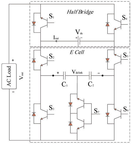
Figure 1.
Nine−Level PEC Inverter Circuit.
Through this layout, the capacitors are arranged horizontally, and an extra DC link is built to guarantee a balanced voltage across the capacitors. A unique technique using signal builder modules is developed in [18] to control the switching states for nine-level generation. Two signal builders—one for charging the capacitors and the other for discharging them alternately regulate the DC link voltage. This continues until the DC link voltage approaches fifty percent of the DC source voltage, with the voltage capacitors being maintained at twenty-five percent of the DC source voltage. Simulation outcomes validate the efficient and excellent performance of the designed modulation technique using MATLAB Simulink. A nine-level voltage signal is produced using simple modulation and a shorter computation time after capacitor voltage balancing. Figure 2 and Figure 3 represent the output voltage waveform and current signal as a function of time before and during S1 fault occurrence at 0.1 s. As can be seen, the voltage and current levels drop during fault presence. After a fault occurrence, a flag alarm or alert can be displayed via a monitoring system until the faulty switch is replaced by a healthy one. Only during the S7 fault switch can the PEC inverter still function as a five- or seven-level inverter where a tolerant system can be designed for setting the DC link to half or one-third of the input voltage accordingly. Although the PEC inverter only has the ability to function if there is a failure in S7, identifying defects in all switches, not only S7, is critical to guarantee stability, security, and effectiveness. Firstly, in several power systems, including PEC 9, switches are linked, which indicates that a malfunction in a particular switch might cause unusual current or voltage levels, overloading other components, or might spread across the system, generating more malfunctions in the remaining parts. This has the potential to disturb the system’s balanced electricity distribution. Identifying these failures guarantees that load transmission is steady, avoiding overloading and guaranteeing all system components obtain appropriate electricity. In a PEC inverter, capacitor voltage balancing is accomplished by redundant switching states. As a result, if other switch failures than S7 remain unnoticed, the redundant system may not work as planned, decreasing the system’s failure tolerance. Moreover, although PEC 9 functions with S7’s defect, the overall effectiveness and performance of the power system may be threatened by failures in other switches, resulting in inefficiencies and perhaps harming fragile equipment. Furthermore, several systems include integrated safety mechanisms based on failure detection. Identifying failures in switches other than S7 might result in various safety actions, such as closing particular elements of the system to avoid risks such as fires, short-circuits, or electric shocks. To sum up, precise identification of faults throughout all switches creates a complete diagnostic illustration, allowing for faster and more successful troubleshooting. It aids in determining the fundamental reason for errors, thus, minimizing subsequent failures.
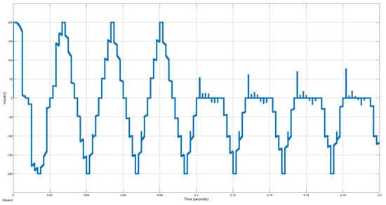
Figure 2.
Output Voltage Waveform before and after S1 Fault at 0.1 s.
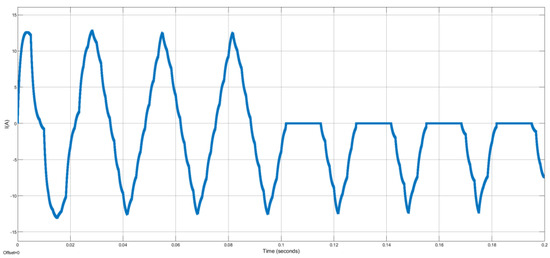
Figure 3.
Output Current Waveform before and after S1 Fault at 0.1 s.
3. Supervised vs. Unsupervised Artificial Intelligence Approaches for Fault Detection
Figure 4 shows the 3D data representation of the chosen features. As can be seen, multiple faults exhibit similar values for these features as they overlap and cannot be easily separated. Actually, not every type of machine learning is deep learning, even though all deep learning involves machine learning. Neural networks with multiple layers, thus, named as deep, are used as a subset of machine learning for analyzing complicated structures in data. Notably, both supervised and unsupervised learning can be used in deep learning. The first step involves feeding the algorithm a paired dataset that consists of a sample and its label. These inputs are also known as instances or findings to be classified. The algorithm, on the other hand, operates in an unsupervised way whenever datasets are not labeled, i.e., the output categorization, computation, and implementation are carried out in the absence of previously defined features.
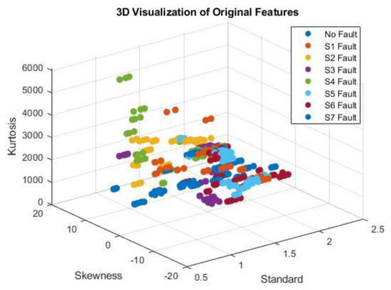
Figure 4.
Three−dimensional Data Visualization of The Three Selected Features.
Despite the fact that unsupervised learning is more effective in finding novel patterns and connections in unlabeled, raw data; nevertheless, a number of obstacles still exist. A number of unsupervised intelligence techniques have been applied to the data gathered from the inverter that is being studied. Unfortunately, employing Gaussian Mixture Models, which calculate the likelihood to which a given data point belongs to a cluster, or Auto-encoders with Clustering or Self-Organizing Maps, which re-represent high dimensional points in a reduced dimensional region, have resulted in inadequate results.
On the other hand, numerous unsupervised structures have been addressed in studies, where each architecture is applied according to data type. Recurrent Neural Networks, Long Short-Term Memory, and Gated Recurrent Unit networks work well for time-varying and consecutive data types [19,20,21,22,23,24,25]. Convolutional Neural Networks are frequently employed for image-based or geographical data, particularly when combined with spectrograms or thermal images [26,27,28,29,30,31]. On the other hand, Deep Belief Networks and Deep Fully Connected Networks are appropriate for large-scale or complicated feature structures [32,33,34]. Thus, supervised machine learning approaches were the main focus of this paper. An effective strategy for learning sophisticated features is attained using the FFNN technique, as it offers simplicity in implementation. Also, RFDT is applied due to its robustness, accuracy, and quick identification. These two techniques have illustrated optimum results in fault diagnosis cases. Hence, this paper contributes to improving the effectiveness of fault detection mechanisms in PEC inverters in which a comparison between ML approaches using the RFDT strategy and deep learning using FFNN for fault detection of single OC switch fault is demonstrated.
4. Proposed Fault Detection Strategy
Figure 5 illustrates the suggested fault detection approach. The voltage produced from the output at the load is created after running the multilevel inverter. A Wavelet Transform (WT) is then used to derive features, and statistical indicators are then calculated. These features are used as input labels for the classifier model, and the switch number associated with the failure is considered the output label. Eventually, using the trained model, estimation and identification of faults are accomplished. The fault detection strategy in this work is designed to ensure reliable, real-time, and precise detection of OC switch failures in PEC inverters. This strategy detects faults early thereby preventing catastrophic breakdown and operational disruption. Moreover, employing WT as well as AI classifiers makes the fault detection strategy more accurate. On the other hand, unlike conventional methods, this approach functions well under various load conditions, which makes it useful for practical uses.

Figure 5.
Flow Chart of Proposed Fault Detection Strategy.
5. Methodology
5.1. Data Preparation and Processing
5.1.1. Data Generation and Simulation Setup
Once an electrical switch encounters an OC failure, it causes unanticipated deformities in the voltage and current signals. As mentioned before, the generated current is impacted by load variations that can result in incorrect categorization. Hence, the produced output voltage is a more trustworthy characteristic for detecting defects as it remains uninfluenced by fluctuations in load. As demonstrated in Figure 6, this study investigates 24 different load levels, with each load consisting of eight no-fault states and one with a single defective switch. Each state’s output voltage is recorded, yielding 192 dataset points.
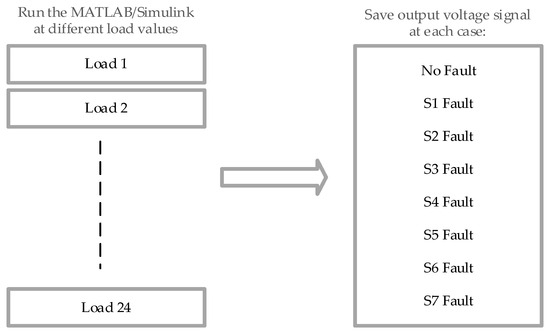
Figure 6.
Data Generation Diagram.
The resistive and inductive load ranges employed in the presented investigation are illustrated in Table 1. They have been specifically selected to resemble high-power electrical appliances frequently encountered in commercial and industrial settings. Large solenoid valves, heavy-duty motors (such as ceiling fans and induction cooktops), industrial electromagnets, and high-capacity transformers generally exhibit electrical behaviors typically observed at these levels. For example, load combinations such as (5 Omega) with (2 H) and (10 Omega) with (10 H) precisely represent the properties of significant industrial electromagnets and magnetic lifting devices, respectively. Likewise, combinations like (2 Omega) with (1.5 H) and (6 Omega) with (1 H) are typical of ceiling fan motors and industrial relay coils. The analysis investigated in this study ensures practical significance and effectiveness for real-world high-power systems. The inclusion of realistic load characteristics enhances the validity and reliability of the results.

Table 1.
Load Values Selected in this study.
5.1.2. Wavelet Transform for Feature Extraction
Using the WT, a signal can be decomposed into its frequency components. It can be divided into two primary categories: Discrete WT and Continuous WT. The latter offers a comprehensive depiction of waveforms whereas DWT divides the signal into groups. The DWT is used in this work as it is especially ideal for tasks such as feature extraction, compression, denoising, and examining the statistical properties of wavelet coefficients. Both approximate and detailed coefficients are obtained during wavelet decomposition. The detailed coefficients preserve thinner, high-frequency information, whereas the approximate coefficients offer a broader, smoothed representation of the data [19,20,21,22,23,24,25,26,27,28,29,30,31,32,33,34,35,36,37,38,39]. This study uses the Daubechies wavelet “db4” to perform a detailed coefficient for the output voltage. In particular, only one level of decomposition is used, deriving the primary set of detail coefficients.
5.1.3. Feature Selection
Mean and standard deviation are widely used as statistical metrics in basic linear analysis. Nevertheless, its reliability increases in unequal and non-linear scenarios. As a result, skewness and kurtosis, which describe the lack of symmetry and the extent of outliers, are more effective statistical metrics for frequency analysis. For example, in articles [40,41,42,43], researchers highlighted the importance of using kurtosis and skewness for recognizing defects to have feasible and reliable fault identification.
The feature selection approach employed is determined by the dataset’s specific characteristics as well as the study’s aims. Evaluating the dataset and choosing a suitable feature selection strategy based on its properties is critical. There are several ways for picking characteristics, each having advantages and disadvantages. To begin with, non-linear transformation aims to extract more meaningful features that better represent the underlying patterns related to faults. It is based on altering the feature space to enhance model learning in the presence of non-linear relationships between features and faults, which is not the case in this work. On the other hand, the filter method assesses each characteristic independently and picks the most significant aspects using statistical metrics such as correlation and shared knowledge. Although filtering algorithms are fast and straightforward, they may not consider relationships between features and may be ineffective with large datasets. In contrast, the wrapper technique employs an algorithm for learning to assess the utility of each portion of the functions. Wrapper techniques are considerably significantly more computationally expensive than filter techniques, but they consider relationships between features and may perform better in datasets with large dimensions. However, they are more susceptible to excess fitting and may be affected by the learning method used. Random Forest Elimination (RFE) has a distinct advantage over filter and wrapper approaches due to the fact that it takes into account the significance, redundant operation, and relationship between features. RFE can successfully decrease the overall size of an information set by iteratively deleting the least significant features while keeping those with the most informative characteristics. Nevertheless, RFE can be computationally demanding, making it unsuitable for large datasets. Nonetheless, Principal Component Analysis (PCA) converts attributes into a space with little dimension that contains the most relevant information. PCA is a great method for reducing the overall size of data and eliminating duplicate features. However, it may lose the interpretation of the original features and may not be appropriate for non-linear correlations between attributes. Thus, RFE identifies the most significant elements that are crucial to a classification model’s prediction ability. RFE with a predetermined number of features to pick is used. This technique creates a model utilizing the rest of the attributes after repeatedly discarding part of the features. The highest retrieved accuracy of the model based on selected features are particularly relevant for predicting the target feature. For example, researchers in [44,45] used the RFE method to pick a meaningful and crucial set of characteristics, resulting in appropriate classification. As a result, numerous iterations with varying numbers of features chosen are performed in which the accuracy of each iteration is captured. This determines how choosing features affected the model’s efficiency throughout iterations. Simulation findings demonstrate that selecting three or four features produces a similar average accuracy of 65%. However, as seen in Figure 7, using three features led to greater accuracy in some cases than utilizing four features. Thus, standard deviation, skewness, and kurtosis are regarded as significant.
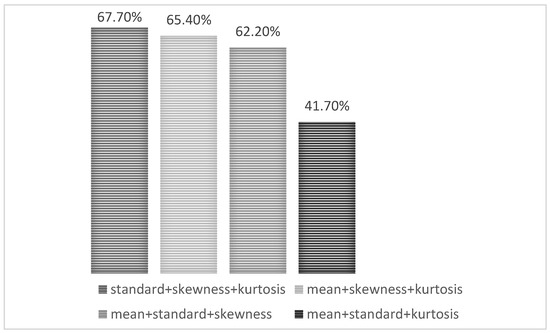
Figure 7.
Histogram Showing Model Accuracy as Function of Different Feature Selection.
5.1.4. Data Augmentation and Preprocessing
Data augmentation is the process of intentionally producing fresh data for training by either using novel fabricated data generated from existing information or inserting substantially altered duplicates of existing datasets. This approach enhances accuracy, reduces overfitting, and strengthens the model’s generalization capability. This leads to considerably more reliable machine learning models [46,47] especially in scenarios with limited data, by introducing alterations that the model might encounter in real-world situations. At first, establish parameters such as the quantity of samples to match to the size of the features. Then, set the augmentation factor, which is adjusted to 2 to twice the dataset as needed. There are numerous sorts of noise that could be advantageous if they properly convey probable perturbations or irregularities in system. For instance, uniform noise introduces persistent random variations, salt and pepper noise introduces abrupt spikes, and speckle noise amplifies noise in relation to the data value. Nevertheless, adding severe or sophisticated noise categories could result in overestimated data that do not accurately represent realistic operations, which may negatively impact the efficiency of the model. Gaussian noise is the most practical option as it realistically simulates measurement errors and operational variability in electrical signals. As Gaussian noise closely resembles natural variations and sensor noise that arise in real-world circumstances. It is typically an effective option for augmenting data in systems requiring high-power electrical equipment. Gaussian noise preserves the system’s fundamental physical properties by introducing tiny, inconsistencies that are centered on the original data. Hence, Gaussian noise with a standard deviation of 0.05 was added to the basic set of features within the scope of data augmentation to improve the classification model’s reliability and generalization ability. In order to replicate the fluctuations and measurement irregularities that can arise in high-power electrical systems in real-life situations, this method was selected. The chosen noise value of 0.05 ensures that the enhanced data maintain meaningful and credible by maintaining the fundamental data framework and adding enough deviations. The predictive algorithm becomes vulnerable to a greater variety of possible scenarios for operations by tripling the dataset with this managed noise injection, which enhances its capacity to reliably differentiate between fault and no-fault states in real-world applications. The noisy version of the features is calculated after noise calculation by applying this equation:
Assuming 3 features (Standard, Skewness, and Kurtosis) and then obtaining updated features in which:
Thus, the feature data for each state are tripled from 24 to 72, resulting in a total of 576 dataset points.
5.1.5. Min-Max Normalization
Normalization is a scaling method in machine learning that is used during data collection. Its goal is to adjust the numbers of numeric columns in the dataset so that they utilize the same scale. It is not required for each dataset in a model. It is only necessary when the features of machine learning models have distinct ranges. Though there are various feature normalization approaches in machine learning, the min-max scaling method is used in this paper. Applying this technique, the dataset is shifted and rescaled to end up ranging between 0 and 1 using this equation:
In which = Value of Normalization; = Maximum value of a feature; = Minimum value of a feature
- Case 1: If the value of X is minimum, the value of Numerator will be 0; hence Normalization will also be 0.
- Case 2: If the value of X is maximum, then the value of the numerator is equal to the denominator; hence normalization will be 1.
- Case 3: On the other hand, if the value of X is neither maximum nor minimum, then values of normalization will also be between 0 and 1.
5.2. Model Development
5.2.1. Random Forest Decision Tree Classifier
This group employs sequential graphs. Its primary idea is to use basic decision rules, which can be learned from training data to predict the class of the target variable. Each possible outcome is considered from top to bottom to make the ultimate decision. The DT approach has demonstrated superior results in the diagnosis of OC switch faults [48] considering its optimal accuracy, robustness, and quick identification period of time.
To produce accurate estimations, increase accuracy, and lessen overlapping, the RF approach remotely builds several DT and aggregates the estimates in a similar way. Additionally, it employs random sampling by employing distinct datasets during the tree-building process and choosing features for each tree randomly. The retrieved voltage signal was used as input for training several machine learning algorithms in the [49], and optimum key matrices were used to assess each algorithm’s functionality. Simulation results have verified the efficacy of the RFDT classifier as it can identify the faulty switch with high robustness and accuracy. The results not only validate the effectiveness of the proposed methodology but also highlight the potential for its practical application in real-world scenarios. Figure 8 demonstrates the architecture of RFDT model having multiple decision trees each having different dataset groups to obtain a final result based on weighted majority voting.
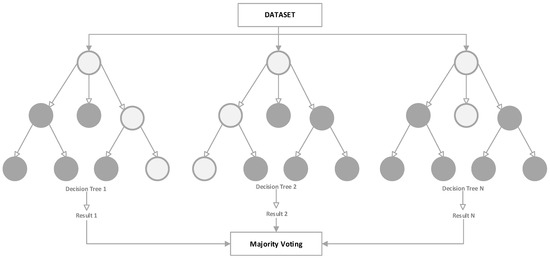
Figure 8.
RFDT Architecture.
5.2.2. Feed-Forward Neural Network Model
FFNN and Back Propagation Neural Network (BPNN) are the two most commonly used varieties regarding supervised neural network strategies. Within the FFNN type, the input array proceeds via the first layer, whose output values constitute the input vector for the following layer. Similarly, the output of the preceding layer generates the input vector of the layer that comes after. This process repeats up until the network outputs the results of the last layer; the more layers there are, the more deeply the data become learned to reveal complicated patterns and correlations. For instance, to identify OC switch faults for cascaded H-Bridge MLIs, the authors in [50] implemented an Artificial Neural Networks (ANN) based on an FFNN type after using a feature extraction procedure by multi-resolution wavelet analysis. However, there are two primary operations in the BPNN category, which are forwarding propagation of signals and back propagation of errors. The training feed-forward network can be expanded in reverse, having error computation functioning as the basic principle of BPNN. Initially, the difference between the actual and predicted amounts by the network is calculated. The goal is to reduce the neural network error by recalculating the weight values in each layer, starting with the last and working backwards to the first layer. Additionally, the gradient descent approach is used to train BPNN in order to modify the neural network’s weight. Authors in the literature have provided several examples of fault diagnosis for OC switches by choosing voltage characteristics for BPNN training [51,52]. Unfortunately, BPNN has a weakness in that it has a slow convergence time and quickly collapses into a local minimum level. As a result, FFNN is used due to its easy implementation and efficient training.
FFNN is a type of ANN where connections between nodes do not form cycles. In simple terms, the data flow in one direction, from input to output. Figure 9 depicts the structure of the neural network designed for detecting and diagnosing faults in inverters. The architecture of neural network consists of an input layer comprising three feature inputs as mentioned earlier, hidden layers comprising a certain number of neurons to be specified later, and an output layer comprising eight predictable outputs corresponding to the number of switch defects and no-fault case. The main idea of the neural network is to create predictions in accordance with the current weights and biases following these steps:
- Input Layers: The input layer receives the scaled data that have been retrieved. After that, weights are employed as the data are transmitted through each hidden layer.
- Hidden Layers: After executing multiple simulations using various transfer functions in hidden layers, the activation function for hidden layers in this paper is set to “tansig”, a hyperbolic tangent sigmoid function required for establishing uncertainty at every single layer and to identify the output of each neuron.
- Output Layer: The network’s estimate is provided by the output layer once the information that was analyzed has been delivered.
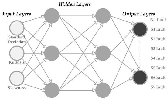
Figure 9.
Architecture of Feed-Forward Neural Network Method.
5.3. Training and Validation Strategy
Training a classifier, assessing its effectiveness, and storing the model for the detection stage are the main objectives of this section. First, the scaled dataset is uploaded, and the grp2idx function is used to transform the categorical labels to numeric labels for additional analysis. The data only in the FFNN method are then shuffled to create random indices for splitting. Then, the data are subsequently divided into two sets: 70% for training and 30% for validation.
5.3.1. Random Forest Decision Tree Model Training and Validation
The template Tree in which a Gradient Boosting (GB) machine classifier is trained. Figure 10 illustrates a flow chart for training the RFDT model. Each new tree in the series is trained to resolve the errors that occurred in the ones preceding it, with an emphasis on instances from prior trees that were incorrectly classified. The objective is to create trees that gradually decrease errors in order to continuously decrease the loss function. Standard RF bagging (parallel learning), in which every tree is a standalone entity, is not the same as this method of successive learning of trees. GB, on the other hand, concentrates on errors and develops over preceding cycles to create a robust model. Moreover, GB not only minimizes overfitting but also is more able to resist slight alterations in data. Also, GB shows optimum operation on small to medium datasets, thereby making it best suitable for the dataset size used in this research. On the other hand, although the AdaBoost process minimizes bias, it is more subject to outliers. Also, although XGBoost is characterized by its rapid and optimized boosting, it still has to be adjusted carefully. Hence, GB is employed in this work to enhance the performance of the RFDT model because of its high precision and robustness. The parameters specified in Table 2 are considered for the RF Classifier. The number of splits is specified to a certain value to manage the tree’s depth, thereby minimizing the level of complexity. As well as avoiding overlapping. Moreover, the towing criterion focuses on attempting to more clearly divide classes by optimizing the disparity between groups produced by the split. This affects the classifier’s capability to manage unbalanced or multiclass data. On the other hand, surrogate splits allow each tree to manage missing data more successfully. This makes the model more robust to missing values, in which alternative split features act as stand-ins when necessary. Moreover, “MergeLeaves = on” points out that leaves that do not significantly enhance the final estimate are merged, thereby minimizing overlapping.
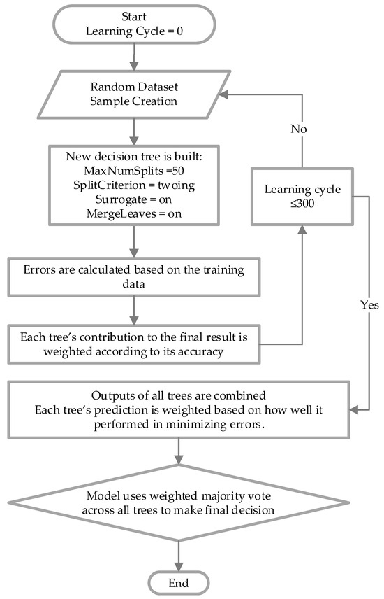
Figure 10.
Flow Chart Showing RFDT Model Training.
Table 2.
Parameters used for RFDT Model Classifier.
5.3.2. Feed-Forward Neural Network Model Training and Validation
Regarding the learning process, the Levenberg–Marquardt (LM) algorithm, executed in MATLAB as “trainlm”, is generally considered an effective training technique, particularly for small to medium-sized networks since it captures additional information about the error surface. It overcomes the issue caused by rapid convergence through integrating elements of the Gauss–Newton and gradient descent approaches. Combining the advantages of both the Gauss–Newton approach and gradient descent, LM adjusts the weights by resolving a non-linear least-squares issue instead of utilizing basic gradient descent. This requires calculating a Jacobian matrix and applying it to more efficiently modify weights for complicated, non-linear error situations. For optimal model performance as well as learning effectiveness, a number of conditions are crucial. First, a key factor in the model’s effectiveness is the actual number of hidden layers. Narrower networks (1–2 layers) are typically preferable for the dataset used in this article since deeper networks with smaller datasets are more likely to overfit when trained. As a result, the network model employs only two hidden layers. The number of neurons that make up each hidden layer is similarly essential. For a variety of classification problems, hidden layers containing 10–50 neurons are frequently essential for preventing overfitting during training. Additionally, when training neural networks with the LM algorithm, four important parameters should be adjusted to maximize model performance: learning rate, maximum number of training epochs, maximum validation failures, and regularization parameter. Learning speed, convergence stability, and network generalization are all influenced by these characteristics. To begin with, the maximum number of epochs (trainParam.epochs) sets the maximum number of training iterations (epochs) as the default value of 1000. The number of consecutive validations allowable before early stopping is accordingly limited to 50 using the maximum validation failures (trainParam.max_fail) parameter. Additionally, the weight update’s step size is controlled by the learning rate. A reduced learning rate strengthens training but necessitates numerous iterations; however, an increased learning rate accelerates the training process but runs the risk of surpassing the required level of accuracy. As a result, a learning rate range between 1 × 10⁻⁴ and 1 × 10⁻¹ is selected. Moreover, the regularization parameter is crucial for creating strong models that adapt effectively to freshly acquired data. Though bigger values (which enforce more weight decay) might lessen overlapping, smaller values have less influence on weights and maintain adaptability. Therefore, the range of the regularization parameter between 1 × 10⁻⁵ and 1 × 10⁻¹ is selected.
Bayesian Optimization for Model Enhancement
Improving the effectiveness of machine learning techniques requires optimizing hyperparameters. The powerful optimization method known as BO develops a probabilistic model of the target function and chooses the most appealing fields to investigate to effectively find the ideal hyperparameters. The BO process is characterized by many factors. In contrast to Particle Swarm Optimization (PSO) and Salp Swarm Algorithm (SSA), which randomly sample hyperparameters, BO employs a surrogate model, commonly a Gaussian Process, to establish a balance between exploration and exploitation. Also, BO successfully avoids local minima in contrast to gradient-based techniques by simulating the state of uncertainty. As BO gives importance to more potential parts of the hyperparameter space, it converges more quickly than PSO and SSA. Moreover, as deep learning model training may suffer from high computations, BO reduces pointless calculations by concentrating exclusively on valuable evaluations in contrast to PSO and SSA, which require many iterations.
Figure 11 demonstrates the Bayesian optimization process implemented. Initially, the ranges for hyperparameters such as neuron number in each hidden layer, learning rate, and regularization are defined. Then, the optimization procedure iterates finding the best parameters that minimize validation error. During each iteration, a neural network is trained using the LM algorithm with early stopping to prevent overfitting; if the model’s validation error does not decrease after a number of checks, the training process stops, and the best weights are retained. After that, Bayesian optimization uses the results from each iteration to select new parameters, continuing this loop until reaching the maximum iterations or the lowest validation error. Ultimately, simulation results of this process yield the optimal parameters presented in Table 3 leading to the minimum validation error utilizing two hidden layers, the first with 43 neurons and the second with 46 neurons. Figure 12 shows the loss function reducing as BO progresses over iterations.
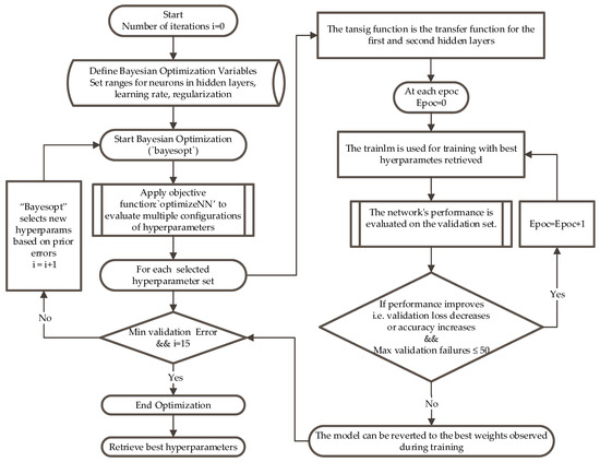
Figure 11.
Flow Chart of Optimization and Training of FFNN Model.
Table 3.
Parameter Used for FFNN Each Model Classifier.
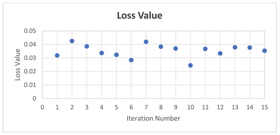
Figure 12.
Loss Value as a Function of Iteration Number during BO Process.
Once the training process ends, the neural network training process, the error histogram, and performance graph during training and validation resulted in Simulink are presented in Figure 13, Figure 14, and Figure 15, respectively. Error variations for two datasets are shown: training and validation. From the above two figures, it is evident that when neural network is adopted for fault detection, an error of order 0.05 is achieved in most of the cases as shown in histogram. It is shown that the error decreases considerably at the end of the training process. The total number of iterations for training of neural network is around 231 as seen in Figure 13, when the maximum validation failures reach 50. Moreover, time taken for training phase is 10 min 14 s. The error rate is minimized and reaches 2.1632 × 10⁻² at iteration 181 during validation after which the error starts increasing.
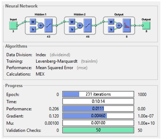
Figure 13.
Neural Network Training Process.
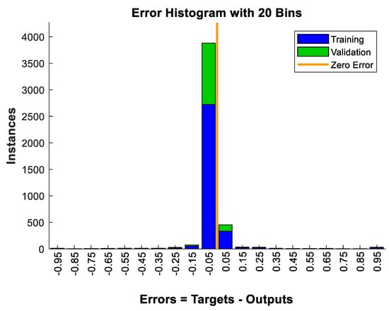
Figure 14.
Error Histogram of the Neural Network during Training and Validation.
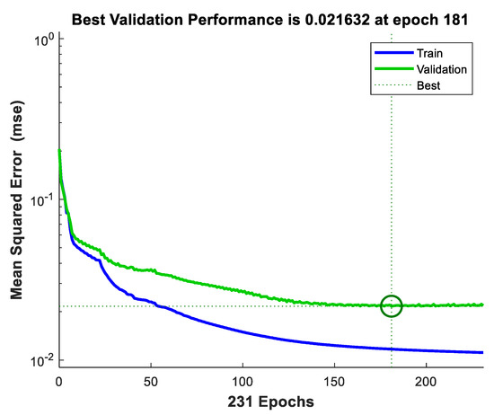
Figure 15.
Performance Graph of Neural Network during Training and Validation.
6. Evaluation Performance Metrics
The validation data are passed through the network to obtain predictions, which are converted back to class labels. Then, the accuracy on the validation set is calculated by comparing predicted values with the true labels. However, this is not enough in deep learning systems; thus, researchers have proposed specific criteria for evaluating classifier performance as follows:
6.1. Confusion Matrix Analysis
In a binary assessment problem, a system of classification assigns a positive or negative rating to events. Combination tables of data, commonly referred to as confusion matrices, are a particular kind of configuration that can illustrate the extent to which a classifier works. They offer an arrangement of every result of the prediction and outcomes of a classification issue and contribute the visualization of its consequences. As seen in Figure 16, a table is displayed showing every classifier’s expected and true value. There are four different categories in the confusion matrix:
- True Positive (TP): The frequency at which the real positive values match the expected positive values from the model classifier;
- False Positive (FP): The frequency at which the model classifier incorrectly expects positive values, but in reality, it is actually negative, i.e., the classifier predicts a positive value, and it is actually negative. It is referred to as Type I error;
- True Negative (TN): The frequency at which real negative values match the expected negative values from the model classifier, i.e., the classifier predicts a negative value, and it is actually negative;
- False Negative (FN): The frequency at which the model classifier incorrectly predicts negative values, but they are in reality positives, i.e., the classifier predicts a negative value, and it is actually positive. It is referred to as a Type II error.
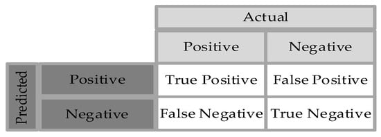
Figure 16.
Confusion Matrix.
A deeper understanding of the model’s recall, accuracy, precision, and entire efficacy in fault classification is made possible by these predictions.
- Accuracy: The model’s accuracy is utilized to assess its performance. It can be expressed as the proportion of all true incidents to all occurrences.
- Precision: The correctness of the model’s positive expectations is determined by its precision. It is expressed as the proportion of TP cases to all of the model’s true and false positive expected cases.
- Recall: A classifier model’s recall determines the extent to which it can locate each significant occurrence throughout a dataset. It is the proportion of TP cases to the total of FN and TP cases.
6.2. Receiver Operator Characteristic (ROC) Curve
It is an additional instrument used to visually assess a classification model’s operation. This is made through showing the extent the number of accurately determined positive cases varying with the number of inaccurately categorized negative instances. Plotting the TP rate, sometimes referred to as recall or sensitivity, against the FP rate at various threshold levels is what the ROC curve does.
6.3. Precision–Recall (PR) Curve
It is an additional visual representation of a classification model’s effectiveness at various thresholds. The PR curve demonstrates the degree to which a predictive model effectively combines precision and recall throughout different decision thresholds by illustrating precision versus recall values.
6.4. Log Loss Metric
A measurement of the extent to how model’s probability prediction’s function is called log loss, also known as cross-entropy loss. By calculating the difference between the predicted and real probabilities, it examines how well the real group classifications fit the expected ones. It can be conceptualized as the negative log-likelihood of the current labels considering the predicted probabilities.
7. Simulation Results and Discussion
After finishing the training of the two classifier models, each model is tested using accuracy, log loss value, confusion matrix, ROC, and PR curves. Table 4 shows the accuracy of RFDT (93%) and FFNN (90%), demonstrating strong performance for both models. In fact, the accuracy of fault identification in this work is relatively high due to several important considerations. Initially, tuning wavelet coefficients makes the extracted features thoroughly represented. Also, a balanced level of noise as well as optimum hyperparameter selection in RFDT or FFNN have increased the accuracy level. To study the model’s performance deeply, the calculated log loss value is considered to be 0.72 for the FFNN model, which is greater than 0.56 for the RFDT model. A lower log-loss value indicates that the predicted probability closely aligns with the actual value, demonstrating the superior performance of the RFDT model. This difference is more clarified through analyzing ROC and PR curves for RFDT and FFNN models below.
Table 4.
Comparison Table Showing Accuracy for Each Model Classifier.
Furthermore, Table 5 shows the confusion matrix for the two examined models. The most essential factor in the confusion matrix is the diagonal elements illustrating the truly predicted samples. For example, a total of 160 samples for the RDFT model and 155 for the FFNN model were correctly predicted out of the total 172 samples and 173 samples, respectively.
Table 5.
Comparison Table Showing Confusion Matrix for Each Model Classifier.
Figure 17 demonstrates ROC curves of the trained classifiers FFNN model and RFDT model. As mentioned above, ROC illustrates the degree to which the total count of correctly identified positive examples fluctuates in relation to the quantity of incorrectly classified negative cases. The ideal ROC curve is one that remains close to the upper-left corner. This demonstrates that the model minimizes false positives while effectively recognizing positive cases. As a result, increasing FP rate and moving towards the right side of the ROC plot typically denotes deteriorating functionality of the model as the number of false positives rises. For most classes, the two curves remain close to the upper left, signifying a high TP rate and a low FP rate. In general, this signifies that both models accomplish a good job in differentiating each category. In contrast to the FFNN graph, the RFDT ROC curve appears to be even more concentrated on the left side of the figure, resulting in a marginally lower FP rate across many classes, which reflects a preferable result. This behavior could point to a general enhancement in minimizing FP. The fault detection model RFDT might additionally manage all categories with greater consistency, as it seems to operate more regularly across classes with minor variances. Conversely, some classes exhibit a bit more fluctuation in the FFNN graph, with a minor decrease in TP rate or increase in FP rate for particular classes.
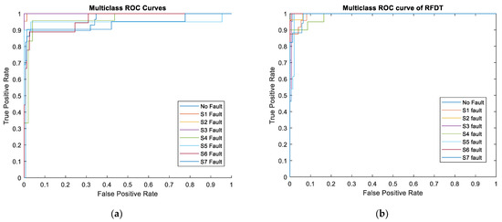
Figure 17.
Graph Showing ROC Curve of (a) Trained Classifier FFNN Model; (b) RFDT Model.
Despite the fact that the ROC curve may present an excessively optimistic picture of the model’s performance, the PR curve more accurately depicts the effectiveness of the positive class in particular. The accuracy of the model’s positive predictions is determined by precision, in which high precision points out that the model gives true positive values more than false positive ones. On the other hand, recall establishes how well a model can identify each faulty state in a dataset. Regarding the overall curve forming illustrated in Figure 18, although the FFNN model begins with decreased precision at decreased recall values, it still reaches a high precision value as the recall value ascends. Nonetheless, the RFDT model typically performs with greater consistency across fault classes, preserving good precision over a broader variety of recall levels. Compared to the FFNN curves, the majority of fault classes in the RFDT curves accomplish precision levels (near 1) throughout a greater portion of the recall spectrum. This implies that RFDT could operate more uniformly across fault types. The FFNN may be less reliable at managing any failure type efficiently because its precision fluctuates considerably across faulty categories according to various recall values. Most faulty categories are increasingly nearing a recall of 1, indicating that both models have strong recall capability. As seen in the figures below, as recall values are closer to 1, the RFDT model tends to maintain a greater precision value, whereas the FFNN model’s precision sharply declines in some faulty categories. Therefore, it indicates that the RFDT functions significantly when it comes to preserving excellent recall as well as excellent precision levels throughout faulty categories.
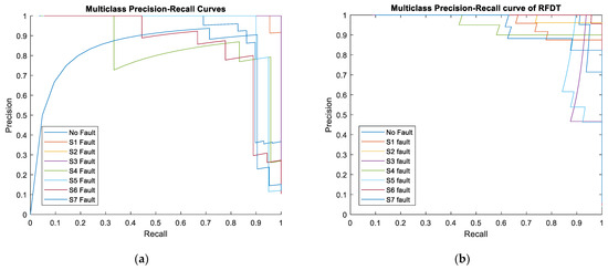
Figure 18.
Graph Showing PR Curve of (a) Trained Classifier FFNN Model; (b) RFDT Model.
In comparison with classifier models employed in [49], Naive Bayes performs least effectively regarding its assumptions about feature independence, especially whenever it deals with correlated features. On the other hand, although K Nearest Neighbors performs rather well, they are perceived to be less reliable, especially when dealing with noisy or unbalanced datasets. Nevertheless, Support Vector Machines (SVM) is a powerful competitor with well-balanced metrics, particularly in terms of accuracy and stability, which makes it appropriate for situations with limited resources. SVM provides a good balance, but it may perform slightly less effectively than FFNN and RFDT in some fault categories, particularly when the FPR is low. It is worth mentioning that FFNN performs exceptionally well based on the ROC and PR curves, showcasing high precision and recall across all fault categories. However, minor variances in the PR curves for particular classes reveal probable areas for optimization, particularly in order to preserve accuracy at very high recall levels. Despite the fact that the time taken for fault detection by the FFNN and RFDT is very fast, around 15 microseconds, it is worth mentioning that training FFNN has taken more time than RFDT, which makes it computationally expensive. Moreover, it requires tuning a large number of parameters. On the contrary, RFDT are faster to train compared to large neural networks, as each decision tree can be built independently. Training complexity scales with the number of trees, but the method is still computationally more efficient than most neural networks. Although FFNN could be enhanced by increasing the number of hidden layers, their learning would be time-consuming and advanced hardware equipment is required. Consequently, the most reliable classifier is RFDT as it exhibits outstanding multiclass ROC performance in every category. This signifies that it would probably attain the highest accuracy for this dataset by preserving excellent precision for the majority of classes at all recall levels. To sum up, RFDT performs outstandingly well in terms of accuracy, stability, and overall performance, making it the optimal classifier by all measures. Thus, RFDT is considered a superior option in this paper, as stability and reliability among every failure type are essential.
8. Conclusions and Future Work
8.1. Findings, Contributions, and Impact
This study contributes to enhancing the reliability and efficiency of fault detection systems in PEC inverters. It demonstrates a comparative analysis of the effectiveness of the RFDT and FFNN methods in accurately identifying OC switch failures in PEC inverters. Initially, features were extracted from the output voltage signal using DWT. Next, both machine learning models were trained using the extracted signal as input. The reliability of the simulation results is verified through utilizing highly accurate and tested models. The outcomes of the simulation are based on well-developed theoretical concepts to verify its consistency and correctness. Extensive testing was carried out under a variety of evaluation criteria to ensure the suggested approach’s resilience and flexibility. Simulation results obtained through MATLAB are considerably reliable due to several factors. Initially, the system being emulated is accurately represented, including logical parameters. Furthermore, the simulation findings are confirmed using optimal key matrices. In summary, the simulation results confirm the superiority of the RFDT classifier, which achieved the highest accuracy (93%), the lowest log loss (0.56), and near-perfect ROC and PR curves, demonstrating exceptional discriminative capability across all fault categories.
8.2. Future Research Directives
MATLAB’s built-in features and toolboxes are highly optimized and validated, ensuring their reliability across various applications. Thus, MATLAB simulations provide comprehensive insights into system operations, ensuring practical applicability. However, future work should execute this strategy on real PEC inverters or other types such as cascaded H-Bridge inverters, T-type inverters, and NPC inverters using embedded systems to validate its real-world functionality. The greater the variety in the dataset, the more generalized the model is; hence, more types of inverters should be simulated to enlarge the dataset knowledge. Although deep learning models achieve high classification accuracy, they require significant computational resources, making implementation on low-power embedded systems challenging.
Author Contributions
Conceptualization, B.M., H.A.S., N.K., H.Y.K. and N.M.; methodology, B.M. and H.A.S.; validation, B.M., H.A.S., N.K., H.Y.K. and N.M.; formal analysis, B.M. and H.A.S.; investigation, B.M.; resources, B.M.; data curation, B.M.; writing—original draft preparation, B.M.; writing—review and editing, B.M. and H.A.S.; visualization, B.M.; supervision, H.A.S., N.K., H.Y.K. and N.M.; project administration, H.A.S., N.K., H.Y.K. and N.M. All authors have read and agreed to the published version of the manuscript.
Funding
This research is funded by the Lebanese University and the Research Council of Saint-Joseph University of Beirut under Project ESIB102.
Data Availability Statement
The raw data supporting the conclusions of this article will be made available by the authors on request.
Acknowledgments
This work has been supported by the Lebanese University and Saint-Joseph University of Beirut joint grant program.
Conflicts of Interest
The authors declare no conflicts of interest.
References
- Yang, S.; Xiang, D.; Bryant, A.; Mawby, P.; Ran, L.; Tavner, P. Condition Monitoring for Device Reliability in Power Electronic Converters: A Review. IEEE Trans. Ind. Electron. 2010, 25, 2734–2752. [Google Scholar] [CrossRef]
- Alavi, M.; Wang, D.; Luo, M. Short-Circuit Fault Diagnosis for Three-Phase Inverters Based on Voltage-Space Patterns. IEEE Trans. Ind. Electron. 2014, 61, 5558–5569. [Google Scholar] [CrossRef]
- Estima, J.O.; Cardoso, A.J.M. A Fault-Tolerant Permanent Magnet Synchronous Motor Drive with Integrated Voltage Source Inverter Open-Circuit Faults Diagnosis. In Proceedings of the 2011 14th European Conference on Power Electronics and Applications, Birmingham, UK, 30 August–1 September 2011; pp. 1–10. [Google Scholar]
- Thantirige, K.; Mukherjee, S.; Zagrodnik, M.A.; Gajanayake, C.; Gupta, A.K.; Panda, S.K. Reliable Detection of Open-Circuit Faults in Cascaded H-Bridge Multilevel Inverter via Current Residual Analysis. In Proceedings of the 2017 IEEE Transportation Electrification Conference (ITEC-India), Pune, India, 13–15 December 2017; pp. 1–6. [Google Scholar] [CrossRef]
- Anand, A.; Akhil, V.B.; Raj, N.; Jagadanand, G.; George, S. An Open Switch Fault Detection Strategy Using Mean Voltage Prediction for Cascaded H-Bridge Multilevel Inverters. In Proceedings of the 2018 IEEE International Conference on Power Electronics, Drives and Energy Systems (PEDES), Chennai, India, 18–21 December 2018; pp. 1–5. [Google Scholar] [CrossRef]
- Anand, A.; Akhil, V.B.; Raj, N.; Jagadanand, G.; George, S. A Generalized Switch Fault Diagnosis for Cascaded H-Bridge Multilevel Inverters Using Mean Voltage Prediction. IEEE Trans. Ind. Appl. 2020, 56, 1563–1574. [Google Scholar] [CrossRef]
- Cheng, S.; Zhao, J.; Chen, C.; Li, K.; Wu, X.; Yu, T.; Yu, Y. An Open-Circuit Fault-Diagnosis Method for Inverters Based on Phase Current. Transp. Saf. Environ. 2020, 2, 148–160. [Google Scholar] [CrossRef]
- Deng, F.; Chen, Z.; Khan, M.R.; Zhu, R. Fault Detection and Localization Method for Modular Multilevel Converters. IEEE Trans. Power Electron. 2015, 30, 2721–2732. [Google Scholar] [CrossRef]
- Li, B.; Shi, S.; Wang, B.; Wang, G.; Wang, W.; Xu, D. Fault Diagnosis and Tolerant Control of Single IGBT Open-Circuit Failure in Modular Multilevel Converters. IEEE Trans. Power Electron. 2016, 31, 3165–3176. [Google Scholar] [CrossRef]
- Xie, D.; Ge, X. A State Estimator-Based Approach for Open-Circuit Fault Diagnosis in Single-Phase Cascaded H-Bridge Rectifiers. IEEE Trans. Ind. Appl. 2019, 55, 1608–1618. [Google Scholar] [CrossRef]
- Masri, B.; Al-Sheikh, H.; Karami, N.; Kanaan, H.; Moubayed, N. A Survey of Open Circuit Switch Fault Diagnosis Techniques for Multilevel Inverters Based on Signal Processing Strategies. In Proceedings of the IEEE 30th International Symposium on Industrial Electronics (ISIE), Kyoto, Japan, 20–23 June 2021; pp. 1–6. [Google Scholar]
- Wang, T.; Xu, H.; Han, J.G.; Elbouchikhi, E.; Benbouzid, M.E.H. Cascaded H-Bridge Multilevel Inverter System Fault Diagnosis Using a PCA and Multiclass Relevance Vector Machine Approach. IEEE Trans. Power Electron. 2015, 30, 7006–7018. [Google Scholar] [CrossRef]
- Cai, B.; Zhao, Y.; Liu, H.; Xie, M. A Data-Driven Fault Diagnosis Methodology in Three-Phase Inverters for PMSM Drive Systems. IEEE Trans. Power Electron. 2017, 32, 5590–5600. [Google Scholar] [CrossRef]
- Yuan, W.; Li, Z.; He, Y.; Cheng, R.; Lu, L.; Ruan, Y. Open-Circuit Fault Diagnosis of NPC Inverter Based on Improved 1-D CNN Network. IEEE Trans. Instrum. Meas. 2022, 71, 1–11. [Google Scholar] [CrossRef]
- Chen, Y.; Sangwongwanich, A.; Huang, M.; Pan, S.; Zha, X.; Wang, H. Failure Risk Assessment of Grid-Connected Inverter with Parametric Uncertainty in LCL Filter. IEEE Trans. Power Electron. 2023, 38, 9514–9525. [Google Scholar] [CrossRef]
- Masri, B.; Al Sheikh, H.; Karami, N.; Kanaan, H.Y.; Moubayed, N. A Review on Artificial Intelligence Based Strategies for Open-Circuit Switch Fault Detection in Multilevel Inverters. In Proceedings of the IECON 2021—47th Annual Conference of the IEEE Industrial Electronics Society, Toronto, ON, Canada, 13–16 October 2021; pp. 1–8. [Google Scholar]
- Sharifzadeh, M.; Al-Haddad, K. Packed E-Cell (PEC) Converter Topology Operation and Experimental Validation. IEEE Access 2019, 7, 93049–93061. [Google Scholar] [CrossRef]
- Masri, B.; Al Sheikh, H.; Karami, N.; Kanaan, H.Y.; Moubayed, N. A Novel Switching Control Technique for a Packed E-Cell (PEC) Inverter Using Signal Builder Block. In Proceedings of the IECON 2022—48th Annual Conference of the IEEE Industrial Electronics Society, Brussels, Belgium, 17–20 October 2022; pp. 1–7. [Google Scholar] [CrossRef]
- Yang, Y.; Haque, M.M.M.; Bai, D.; Tang, W. Fault Diagnosis of Electric Motors Using Deep Learning Algorithms and Its Application: A Review. Energies 2021, 14, 7017. [Google Scholar] [CrossRef]
- Shu, Y.; Xu, Y. End-to-End Captcha Recognition Using Deep CNN-RNN Network. In Proceedings of the 2019 IEEE 3rd Advanced Information Management, Communicates, Electronic and Automation Control Conference (IMCEC), Chongqing, China, 11–13 October 2019; pp. 54–58. [Google Scholar] [CrossRef]
- Renjith, S.; Manazhy, R. Indian Sign Language Recognition: A Comparative Analysis Using CNN and RNN Models. In Proceedings of the 2023 International Conference on Circuit Power and Computing Technologies (ICCPCT), Kollam, India, 22–23 June 2023; pp. 1573–1576. [Google Scholar] [CrossRef]
- Prabowo, Y.D.; Warnars, H.L.H.S.; Budiharto, W.; Kistijantoro, A.I.; Heryadi, Y.; Lukas. LSTM and Simple RNN Comparison in the Problem of Sequence to Sequence on Conversation Data Using Bahasa Indonesia. In Proceedings of the 2018 Indonesian Association for Pattern Recognition International Conference (INAPR), Jakarta, Indonesia, 7–8 October 2018; pp. 51–56. [CrossRef]
- Musadiq, M.S.; Lee, D.-M. A Novel Capacitance Estimation Method of Modular Multilevel Converters for Motor Drives Using Recurrent Neural Networks with Long Short-Term Memory. Energies 2024, 17, 5577. [Google Scholar] [CrossRef]
- Odinsen, E.; Amiri, M.N.; Burheim, O.S.; Lamb, J.J. Estimation of Differential Capacity in Lithium-Ion Batteries Using Machine Learning Approaches. Energies 2024, 17, 4954. [Google Scholar] [CrossRef]
- Bui, L.D.; Nguyen, N.Q.; Doan, B.V.; Riva Sanseverino, E.; Tran, T.T.Q.; Le, T.T.H.; Le, Q.S.; Le, C.T.; Cu, T.T.H. Refining Long Short-Term Memory Neural Network Input Parameters for Enhanced Solar Power Forecasting. Energies 2024, 17, 4174. [Google Scholar] [CrossRef]
- Jiang, A.; Yan, N.; Wang, F.; Huang, H.; Zhu, H.; Wei, B. Visible Image Recognition of Power Transformer Equipment Based on Mask R-CNN. In Proceedings of the 2019 IEEE Sustainable Power and Energy Conference (iSPEC), Beijing, China, 20–23 November 2019; pp. 657–661. [Google Scholar] [CrossRef]
- Kido, S.; Hirano, Y.; Hashimoto, N. Detection and Classification of Lung Abnormalities by Use of Convolutional Neural Network (CNN) and Regions with CNN Features (R-CNN). In Proceedings of the 2018 International Workshop on Advanced Image Technology (IWAIT), Chiang Mai, Thailand, 7–9 January 2018; pp. 1–4. [Google Scholar] [CrossRef]
- Wang, J.; Zhang, X.; Gao, G.; Lv, Y. OP Mask R-CNN: An Advanced Mask R-CNN Network for Cattle Individual Recognition on Large Farms. In Proceedings of the 2023 International Conference on Networking and Network Applications (NaNA), Qingdao, China, 27–29 October 2023; pp. 601–606. [Google Scholar] [CrossRef]
- Serikbay, A.; Bagheri, M.; Zollanvari, A.; Phung, B.T. Ensemble Pretrained Convolutional Neural Networks for the Classification of Insulator Surface Conditions. Energies 2024, 17, 5595. [Google Scholar] [CrossRef]
- Ding, L.; Guo, H.; Bian, L. Convolutional Neural Networks Based on Resonance Demodulation of Vibration Signal for Rolling Bearing Fault Diagnosis in Permanent Magnet Synchronous Motors. Energies 2024, 17, 4334. [Google Scholar] [CrossRef]
- Wang, J.; Li, H.; Wu, C.; Shi, Y.; Zhang, L.; An, Y. State of Health Estimations for Lithium-Ion Batteries Based on MSCNN. Energies 2024, 17, 4220. [Google Scholar] [CrossRef]
- Ren, Y.; Tao, Z.; Zhang, W.; Liu, T. Modeling Hierarchical Spatial and Temporal Patterns of Naturalistic fMRI Volume via Volumetric Deep Belief Network with Neural Architecture Search. In Proceedings of the 2021 IEEE 18th International Symposium on Biomedical Imaging (ISBI), Nice, France, 13–16 April 2021; pp. 130–134. [Google Scholar] [CrossRef]
- Yan, S.; Xia, X. A Method for Predicting the Temperature of Steel Billet Coming Out of Soaking Furnace Based on Deep Belief Neural Network. In Proceedings of the 2024 IEEE 2nd International Conference on Control, Electronics and Computer Technology (IC-CECT), Jilin, China, 26–28 June 2024; pp. 1042–1046. [Google Scholar] [CrossRef]
- Zhang, D.; Chen, S. Insulator Contamination Grade Recognition Using the Deep Learning of Color Information of Images. Energies 2021, 14, 6662. [Google Scholar] [CrossRef]
- Srivani, S.G.; Vyas, U.B. Fault Detection of Switches in Multilevel Inverter Using Wavelet and Neural Network. In Proceedings of the 2017 7th International Conference on Power Systems (ICPS), Pune, India, 21–23 December 2017; pp. 151–156. [Google Scholar]
- Xu, J.; Song, B.; Zhang, J.; Xu, L. A New Approach to Fault Diagnosis of Multilevel Inverter. In Proceedings of the 2018 Chinese Control and Decision Conference (CCDC), Shenyang, China, 9–11 June 2018; pp. 1054–1058. [Google Scholar]
- Chowdhury, M.; Bhattacharya, D.; Khan, M.; Saha, S.; Dasgupta, A. Wavelet Decomposition-Based Fault Detection in Cascaded H-Bridge Multilevel Inverter Using Artificial Neural Network. In Proceedings of the 2017 2nd IEEE International Conference on Recent Trends in Electronics, Information & Communication Technology (RTEICT), Bangalore, India, 19–20 May 2017; pp. 1931–1935. [Google Scholar]
- Lin, P.; Zhang, Z.; Zhang, Z.; Kang, L.; Wang, X. Open-Circuit Fault Diagnosis for Modular Multilevel Converter Using Wavelet Neural Network. In Proceedings of the 2019 IEEE Innovative Smart Grid Technologies—Asia (ISGT Asia), Chengdu, China, 21–24 May 2019; pp. 250–255. [Google Scholar]
- Gomathy, V.; Selvaperumal, S. Fault Detection and Classification with Optimization Techniques for a Three-Phase Single-Inverter Circuit. J. Power Electron. 2016, 16, 1097–1109. [Google Scholar] [CrossRef]
- Amaral, T.G.; Pires, V.F.; Cordeiro, A.; Foito, D. A Skewness-Based Method for Diagnosis in Quasi-Z T-Type Grid-Connected Converters. In Proceedings of the 2019 8th International Conference on Renewable Energy Research and Applications (ICRERA), Brasov, Romania, 3–6 November 2019; pp. 131–136. [Google Scholar] [CrossRef]
- Ozansoy, C. Performance Analysis of Skewness Methods for Asymmetry Detection in High Impedance Faults. IEEE Trans. Power Syst. 2020, 35, 4952–4955. [Google Scholar] [CrossRef]
- Luo, C.; Jia, M.; Wen, Y. The Diagnosis Approach for Rolling Bearing Fault Based on Kurtosis Criterion EMD and Hilbert Envelope Spectrum. In Proceedings of the 2017 IEEE 3rd Information Technology and Mechatronics Engineering Conference (ITOEC), Chongqing, China, 3–5 October 2017; pp. 692–696. [Google Scholar] [CrossRef]
- Zhang, Y.; Zhang, C.; Liu, X.; Wang, W.; Han, Y.; Wu, N. Fault Diagnosis Method of Wind Turbine Bearing Based on Improved Intrinsic Time-Scale Decomposition and Spectral Kurtosis. In Proceedings of the 2019 Eleventh International Conference on Advanced Computational Intelligence (ICACI), Guilin, China, 7–9 June 2019; pp. 29–34. [Google Scholar] [CrossRef]
- Zhang, C.; Li, Y.; Yu, Z.; Tian, F. Feature Selection of Power System Transient Stability Assessment Based on Random Forest and Recursive Feature Elimination. In Proceedings of the 2016 IEEE PES Asia-Pacific Power and Energy Engineering Conference (APPEEC), Xi’an, China, 25–28 October 2016; pp. 1264–1268. [Google Scholar] [CrossRef]
- Choudhury, D.; Bhattacharya, A. Weighted-Guided-Filter-Aided Texture Classification Using Recursive Feature Elimination-Based Fusion of Feature Sets. In Proceedings of the 2015 IEEE International Conference on Computer Graphics, Vision and Information Security (CGVIS), Bhubaneswar, India, 2–3 November 2015; pp. 126–130. [Google Scholar] [CrossRef]
- Mukai, K.; Kumano, S.; Yamasaki, T. Improving Robustness to Out-of-Distribution Data by Frequency-Based Augmentation. In Proceedings of the 2022 IEEE International Conference on Image Processing (ICIP), Bordeaux, France, 16–19 October 2022; pp. 3116–3120. [Google Scholar] [CrossRef]
- Shi, G.; Liu, B.; Walls, L. Data Augmentation to Improve the Performance of Ensemble Learning for System Failure Prediction with Limited Observations. In Proceedings of the 2022 13th International Conference on Reliability, Maintainability, and Safety (ICRMS), Kowloon, Hong Kong, 5–7 September 2022; pp. 296–300. [Google Scholar] [CrossRef]
- Achintya, P.; Sahu, L.K. Open Circuit Switch Fault Detection in Multilevel Inverter Topology Using Machine Learning Techniques. In Proceedings of the 2020 IEEE 9th Power India International Conference (PIICON), Sonepat, India, 28 February–1 March 2020; pp. 1–6. [Google Scholar]
- Masri, B.; Al Sheikh, H.; Karami, N.; Kanaan, H.Y.; Moubayed, N. A Novel Fault Detection Technique for Single Open Circuit in a Packed E-Cell Inverter. In Proceedings of the IECON 2024—50th Annual Conference of the IEEE Industrial Electronics Society, Chicago, IL, USA, 6–9 October 2024; pp. 1–6. [Google Scholar]
- Liu, Z.; Li, C.; Zhang, S. A Principal Components Rearrangement Method for Feature Representation and Its Application to the Fault Diagnosis of CHMI. Energies 2017, 10, 1273. [Google Scholar] [CrossRef]
- Raj, N.; Jagadanand, G.; George, S. Fault Detection and Diagnosis in Asymmetric Multilevel Inverter Using Artificial Neural Network. Int. J. Electron. 2017, 105, 559–571. [Google Scholar] [CrossRef]
- Chen, D.; Liu, Y.; Zhou, J. Optimized Neural Network by Genetic Algorithm and Its Application in Fault Diagnosis of Three-Level Inverter. In Proceedings of the 2019 CAA Symposium on Fault Detection, Supervision and Safety for Technical Processes (SAFEPROCESS), Xiamen, China, 23–26 July 2019; pp. 116–120. [Google Scholar] [CrossRef]
Disclaimer/Publisher’s Note: The statements, opinions and data contained in all publications are solely those of the individual author(s) and contributor(s) and not of MDPI and/or the editor(s). MDPI and/or the editor(s) disclaim responsibility for any injury to people or property resulting from any ideas, methods, instructions or products referred to in the content. |
© 2025 by the authors. Licensee MDPI, Basel, Switzerland. This article is an open access article distributed under the terms and conditions of the Creative Commons Attribution (CC BY) license (https://creativecommons.org/licenses/by/4.0/).