A Flexible Quantification Method for Buildings’ Air Conditioning Based on the Light and Heat Transfer Coefficients: A Case Study of a Shanghai Office Building

Abstract

The massive integration of renewable electricity places significant regulatory pressure on urban power grids. This has also promoted the development of virtual power plant technology. The air conditioning systems of public buildings, as one of the main cores of virtual power plants, have flexible regulation capability that is difficult to quantify accurately, leading to slow development in practical engineering applications. This study proposes quantifying the flexible regulation capability of public building air conditioning systems based on heat and light transfer coefficient (HTC and LTC). Taking a public building in Shanghai as an example, this study combines 3D modeling and simulation and sliding window and correlation analysis techniques to investigate changes in influencing factors under different time periods, levels of insulation performance, and window-to-wall ratios. Drawing an analogy with energy storage batteries, two quantification indicators, response time (RT) and response energy loss (RL), are proposed and combined with heat and light transmission systems for nonlinear fitting. Finally, a sensitivity analysis of the impact of external environment and building performance is conducted. The results of sliding window and correlation analysis show that surface irradiance has the highest correlation with air conditioning energy consumption (over 0.8). However, through linear and nonlinear fitting, it was found that HTC can better characterize the two key indicators of RT and RL in air conditioning flexible adjustment, with fitting degrees (R²) of 80% and 72%, respectively. The results obtained from this study can provide a quantitative reference for quantification and response control research into the flexible regulation capability of public building air conditioning systems.

1. Introduction

To address climate change and achieve a global energy transition, the proportion of renewable energy in the entire energy system is increasing. Due to significant regional and seasonal variations in new energy output, challenges such as power consumption, peak shaving, and frequency modulation are becoming increasingly prominent. To tackle these challenges, various means of peak shaving and frequency modulation have been developed. On the production side, the adoption of advanced energy storage technologies and smart scheduling systems can effectively balance the fluctuations in new energy generation and ensure the stable operation of the power grid. Meanwhile, on the transmission side, optimizing grid structure and improving transmission efficiency can reduce energy loss and enhance the reliability of power transmission. In addition to adjustments on the production and transmission sides, implementing flexible energy use regulation on the demand side is also an extremely important need [1].

Energy-consuming equipment in buildings can intelligently adjust its power consumption based on renewable energy supply conditions and electricity price signals. This dynamic adjustment mechanism is called demand-side response [2]. It can be further divided into energy-consuming devices with regulating capabilities (such as air conditioning, lighting, and electric vehicles) and energy-supply devices (such as energy storage and cogeneration). By changing their own energy consumption patterns and utilizing the ability of demand-side resources to respond quickly, users can reduce or shift the electricity load within a specific time period, thereby optimizing the balance between power supply and demand. This not only helps to reduce energy costs, alleviate the pressure of electricity consumption during peak hours, and improve the utilization rate of renewable energy but also enhances the stability of the entire energy system. Demand-side response promotes the effective management of energy throughout society, not only enhancing the flexibility of energy systems but also promoting more flexible energy utilization in the construction sector [3].

The virtual power plant involving building air conditioning is currently a research hotspot in demand-side response. However, in practical applications, such response actions often result in situations where the adjustable values provided by the user do not match the actual values [4]. In the actual response of the Shanghai power grid in 2024, there was even a deviation of 30–40%. This situation has led to a large number of response strategy studies being unable to be effectively applied due to actual errors. The core reason for this situation is that the building air conditioning system is influenced by the interaction of internal and external factors such as fence structure, climate, and human behavior [5,6] and the difficulty involved in quantitative characterization is complex. Therefore, it is necessary to carry out a quantification of the flexible adjustment capacity of building air conditioning systems to help cluster schedulers to better understand the objects to be scheduled.

1.1. Review of Relevant Research

1.1.1. Factors Affecting the Flexibility of Air Conditioning Systems

The prerequisite for studying the quantification of building air conditioning system flexibility is to clarify the factors that affect air conditioning flexibility. These factors can be divided into two main categories: first, the physical characteristics of the building itself, including the thermal physical properties of the building envelope, the volume of the building, and the building form [7]; and second, weather conditions, which include changes in temperature and humidity during the day, radiation changes, seasonal variations, and differences in temperature zones [8].

In terms of the physical characteristics of buildings themselves, previous research has primarily focused on the impact of typical buildings on energy flexibility, including factors such as building types and insulation performance [9]. Overall, these studies essentially investigate the thermal performance of building envelopes. The insulation performance of an envelope reflects the heat transfer characteristics of a building: better insulation means lower heat loss rates and this is more conducive to energy transfer [7]. Lu et al. [10] studied the impact of the thermal mass of building envelopes on the energy flexibility of buildings during the cooling season and found that greater thermal mass helps to reduce the peak load and improve the energy efficiency of passive energy storage.

The performance of building energy flexibility varies in different external environments, so buildings need to choose appropriate demand-side responses for different weather conditions to achieve energy flexibility [11]. Weather conditions, including the outdoor temperature, relative humidity, outdoor wind speed, and solar radiation, directly impact the energy demand of buildings and consequently alter their energy flexibility [12]. Foteinaki et al. [9] took single-family residential buildings and apartment buildings as research objects, set HVAC temperature regulation parameters within the range of human comfort, and quantified the buildings’ load increase or decrease during the regulation period. Research indicates that energy flexibility is highly correlated with solar radiation, emphasizing the importance of the insulation performance of building envelopes.

1.1.2. Quantitative Characterization of Flexibility in Air Conditioning Systems

Regarding quantitative characterization methods for the flexibility of air conditioners, typical modeling approaches mainly include building models based on heat exchange, load models based on equivalent thermal parameters, and gray-box thermodynamic models. They are usually used to reflect time-varying relationships for the energy consumption of air-conditioning systems, cooling/heating capacities, and room temperatures. Li [13] used a second-order ETP model to simulate a new type of indoor intelligent thermostatic system, which helped to determine the relationship between the ambient temperature and the energy consumption of the air conditioner and improved the accuracy of the thermostatic system. The experimental results showed that, compared to traditional thermostatic systems, this new type of thermostatic system can reduce energy consumption by 11.5%. However, the study still focuses on the application of quantified building performance without further analysis of the intrinsic correlation between building performance, the external environment, and air conditioning energy consumption.

Based on this, flexibility is generally characterized directly or indirectly through software simulation [14] or experiments in specific scenarios to obtain fitting formulas [15]. Arteconia [16] and others have proposed an energy flexibility building identification method, which quantifies AVES using four parameters—response time, committed power, recovery time, and actual energy change—and studied the impacts of climate, building characteristics, and HVAC systems. Both Dreau [17] and Hurtado [8] used EnergyPlus to simulate AVES. The former analyzed the effects of different building characteristics (such as insulation and airtightness), different rooms’ set temperatures, and different heating methods (such as radiators or floor radiant heating). The latter proposed quantification indicators such as response rate, flexible power and capacity, and charge/discharge time.

Additionally, the aggregated flexibility representation of large-scale air conditioning load clusters can be established through methods such as Monte Carlo sampling and self-organizing map neural networks. Hu et al. [18] studied the response potential of residential loads in Hong Kong by establishing a gray-box thermal model. The study showed that this thermal model could reflect the basic thermodynamics of air-conditioned rooms while maintaining a simple structure. Zhang et al. [19] used the Monte Carlo method to perform aggregated calculations on a second-order ETP model, obtaining the baseline load before large-scale air conditioning participation in demand response.

However, their research was limited to the impact of building performance parameters themselves on air conditioning energy consumption and did not interact performance parameters with outdoor environments. This has led to excessive personalization in the above research and the corresponding application of research results needs to meet the dual matching requirements of building performance and external environment, with poor generalization ability. Due to the multiple influences of building performance, external environment, and human behavior on the air conditioning load demand of buildings, the coupling between other building performance and external environment becomes particularly important when human behavior cannot be accurately predicted.

1.2. Content and Contribution

From the existing literature, it can be seen that the factors influencing building air conditioning are divided into two different dimensions: the building itself and the season. The former is a static value determined by the building itself, while the latter is a dynamic value that changes at any time. The difference between these two types of variables also often limits the current quantitative characterization of building air conditioning flexibility to a specific building or region and the quantitative results obtained are difficult to popularize and promote [20,21]. For these reasons, this study proposes a light and heat transfer system that combines the thermal physical properties of the building body with the external dynamic environment. Taking the summer working conditions of a public building in Shanghai as an example, a simulation is conducted using EnergyPlus 24.1.0. Based on the sliding window technique and correlation analysis, the significant impact of building ontology attributes on the external environment can be studied. Through the correlation and regression analysis of thermal and optical transmission coefficients, the effectiveness of the proposed quantification coefficients is studied. Analogous to energy storage batteries, energy attribute indicators such as the response time and response loss of building air conditioning flexibility can be quantitively obtained. Finally, the impact of control details such as precooling time and shutdown time can be analyzed. The main innovations and contributions of this study are as follows:

(1)

A quantitative method for the flexibility of air conditioning systems using heat transfer coefficients and optical transmission systems has been proposed, which can achieve the dynamic quantitative characterization of air conditioning flexibility in public buildings and help to refine the practical implementation of flexible response research;

(2)

Split and combine the two factors that have the greatest impact on building air conditioning energy consumption, namely building performance and external climate. By analyzing the quantitative accuracy of the flexible adjustment capability indicators of air conditioning, the influencing factors and mechanisms of RT and RL indicators were explored, which helps to establish a more reasonable evaluation method for air conditioning flexibility in public buildings.

2. Methodology

2.1. Factor Correlation Analysis Based on the Sliding Window Technique

The analysis of influencing factors includes different methods such as correlation analysis and principal component analysis. Among them, principal component analysis is prone to losing information during dimensionality reduction, resulting in poor interpretability [12]. At the same time, sliding window technology can intuitively see the impact of temporal changes in data. Therefore, this study adopts a combination of sliding window and correlation analysis to analyze the influencing factors of external environment and air conditioning energy consumption. The sliding window technique involves segmenting continuous building performance data into multiple subdatasets based on fixed time intervals, such as hourly or daily. A suitable window size is set (e.g., data from the past week or month) and this window is applied to each subdataset to capture local characteristics and trends in the data [22]. Within each sliding window, key indicators are extracted, such as temperature, humidity, wind speed, etc. [12,23].

Spearman’s rank coefficient of correlation (SCC), also known as the Spearman correlation coefficient, reflects the correlation between the trends and strengths of changes in two random variables, with values ranging between –1 and 1 [24]. For two sets of data, X and Y, the Spearman correlation coefficient is given by the following formula:

$$r_s=1-{\displaystyle \frac{6{\displaystyle \sum _{i=1}^n{d}_i^2}}{n(n^2-1)}}$$

(1)

Here, $d_i$ represents the rank difference between $X_i$ and $Y_i$. A rank is the position of a number after a column of data has been sorted from smallest to largest; if two numbers are equal, their positions are averaged. Both Spearman’s rank correlation coefficient and Pearson’s correlation coefficient are methods for measuring the strength of association between two variables. However, Pearson’s correlation coefficient assumes a linear relationship between variables and requires the data to follow a normal distribution. Spearman’s rank correlation coefficient replaces the actual data values with their rank positions, making it more adept at handling nonlinear and non-normally distributed data while also capable of dealing with linearly related variables, albeit with longer computation times.

The combination of these techniques allows for the capture of local features of the data and for deeper relationships between variables to be analyzed, thereby providing a more comprehensive assessment of the factors influencing air conditioning flexibility in public buildings [24].

2.2. Quantitative Representation Method

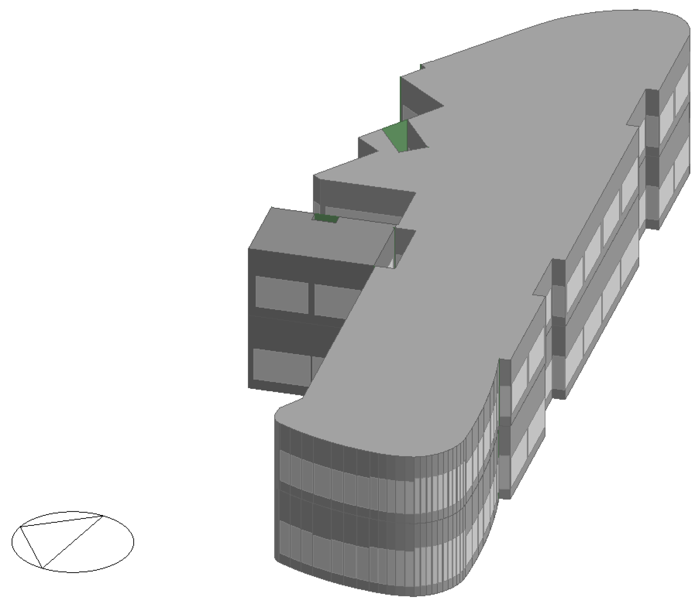
This study proposes two evaluation and quantification indicators for the flexibility of air conditioning in public buildings, namely the heat transfer coefficient (HTC) and the light transfer coefficient (LTC). HTC is the product of weighted heat transfer coefficient and indoor/outdoor temperature difference, measured in °C. The weighted heat transfer coefficient is the weighted heat transfer coefficient of various fence structures such as exterior walls, roofs, windows, etc. based on their area. LTC is the amount of indoor irradiance obtained after considering the window to wall ratio, measured in W/m².

Through the thermal transfer coefficient and the light transmission system, we can draw an analogy with the performance indicators of energy storage batteries to define the energy attribute indicators of the flexibility of public building air conditioning systems, which are response time (RT, hours) and response energy loss (RL, %). The response time can be used for the integral calculation of air conditioning power consumption to obtain the total response electricity. The response loss is the explicit cost of the response process, which, together with implicit costs such as user comfort, constitutes the lower limit of the response object’s quotation. Therefore, by using response time and response loss, it is possible to further calculate all the demand data for the economic interaction between the power grid and the response object.

3. Case Study

The case study for this research is a public building in Shanghai, China, with a construction area of approximately 5000 square meters. The region in which the building is located experiences hot summers and cold winters, leading to a high dependency on the building’s air conditioning system. Correspondingly, the potential for flexible regulation of the air conditioning system in such buildings is also relatively high. In this study, the building was first modeled in three dimensions in REVIT according to the design drawings of the public building, ensuring an accurate division of room functions. The building model was then imported into the energy simulation tool EnergyPlus to obtain an editable building energy simulation case (Figure 1).

At this stage, some basic parameters need to be set, as shown in

Table 1. Simulation model parameter settings.

Building Related Settings
External wall heat transfer coefficient	0.6 (0.2–1.0) (W/m2·K)
Roof heat transfer coefficient	0.4 (W/m2·K)
Household wall, corridor wall heat transfer coefficient	1.5 (W/m2·K)
Doors heat transfer coefficient	2 (W/m2·K)
Windows heat transfer coefficient	2 (W/m2·K)
Window to wall ratio	0.5 (0.2–0.7)
Personnel density	5 (m2/person)
Equipment heat dissipation	12 (W/m2)
Air Conditioning System-Related Settings
Air conditioning opening temperature	28 °C
Air conditioning set temperature	26 °C
Average annual COP of air conditioning system	3.5
Air conditioning system form	Chiller and fan coil unit

below. Among them, the heat transfer coefficient of the building fence structure includes various types such as exterior walls, roofs, windows, doors, corridor walls, etc. In order to reduce the number of control experiments, this article only conducted changes in the external wall heat transfer system (0.2–1.0 (W/m²·K)). It is particularly important to note that the setting of the external wall heat transfer coefficient (0.6 (W/m²·K)) and the window-to-wall ratio (0.5) is for the subsequent correlation analysis of the impact of external climate changes. In the subsequent research on building properties and the light–heat transfer system, the external wall heat transfer coefficient and the window-to-wall ratio will be varied according to the design standards of Chinese buildings over the past 10–20 years [25,26]. In addition, the target illumination set is 150 lux. Normalized power density is 5 (W/m²-100 lux). In terms of ventilation, the air exchange rate is 3 ac/h.

In order to conduct a detailed analysis of the flexible adjustment capability of air conditioning systems in office buildings in Shanghai, we imported climate parameters from Shanghai (temperature, humidity, wind speed, irradiance, etc.). At the same time, the start and stop time of the air conditioner is also independently controlled to ensure immediate shutdown at the required time. According to the simulation results, the annual air conditioning cooling energy consumption of the target office building is 133 MWh, and the air conditioning energy consumption per unit area is 26 (kWh/m²). These data are slightly lower than the average energy consumption of public buildings released by the Shanghai Municipal Government in 2022 (28.6 (kWh/m²)). Due to it being a newly constructed building with a high level of energy efficiency, this falls within the credible range [27]. Meanwhile, compared to the actual test data, the error of the simulation model is controlled within 10%, so it can be considered that the established simulation model has high reliability. As shown in Figure 2, the comparison between simulated data and actual data for five consecutive days from July 15th to 19th is presented. Although the changes in actual data and simulated data are not completely the same due to the influence of actual user behavior, the overall trend can still be maintained in consistency. Meanwhile, in terms of data, during the peak demand period for summer air conditioning from June to August, the error between simulated data and actual data is smaller, for example, the error shown in Figure 2 does not exceed 5%. Therefore, it can be considered that the simulation model obtained in this study exhibits better accuracy during peak air conditioning demand periods when flexible adjustment of air conditioning is more necessary.

Further research will be conducted on this model in the future. Due to the earliest air conditioning load demand in Shanghai occurring in May, in order to fully cover all operating conditions of air conditioning, the overall simulation period spans from 1 May to 1 November, fully covering the peak demand of summer as well as the transitional phases of cold and heat in spring and autumn. After removing the dates when the air conditioning was not turned on, the simulation data were clustered into four typical days using K-means clustering, as shown in Figure 3. Cluster centers 1 and 2 in the figure represent typical air conditioning operation during the transitional season. Cluster center 3 is a regular operating condition during summer. Cluster center 4 reflects the typical daily operating situation of peak demand in summer.

4. Result and Analysis

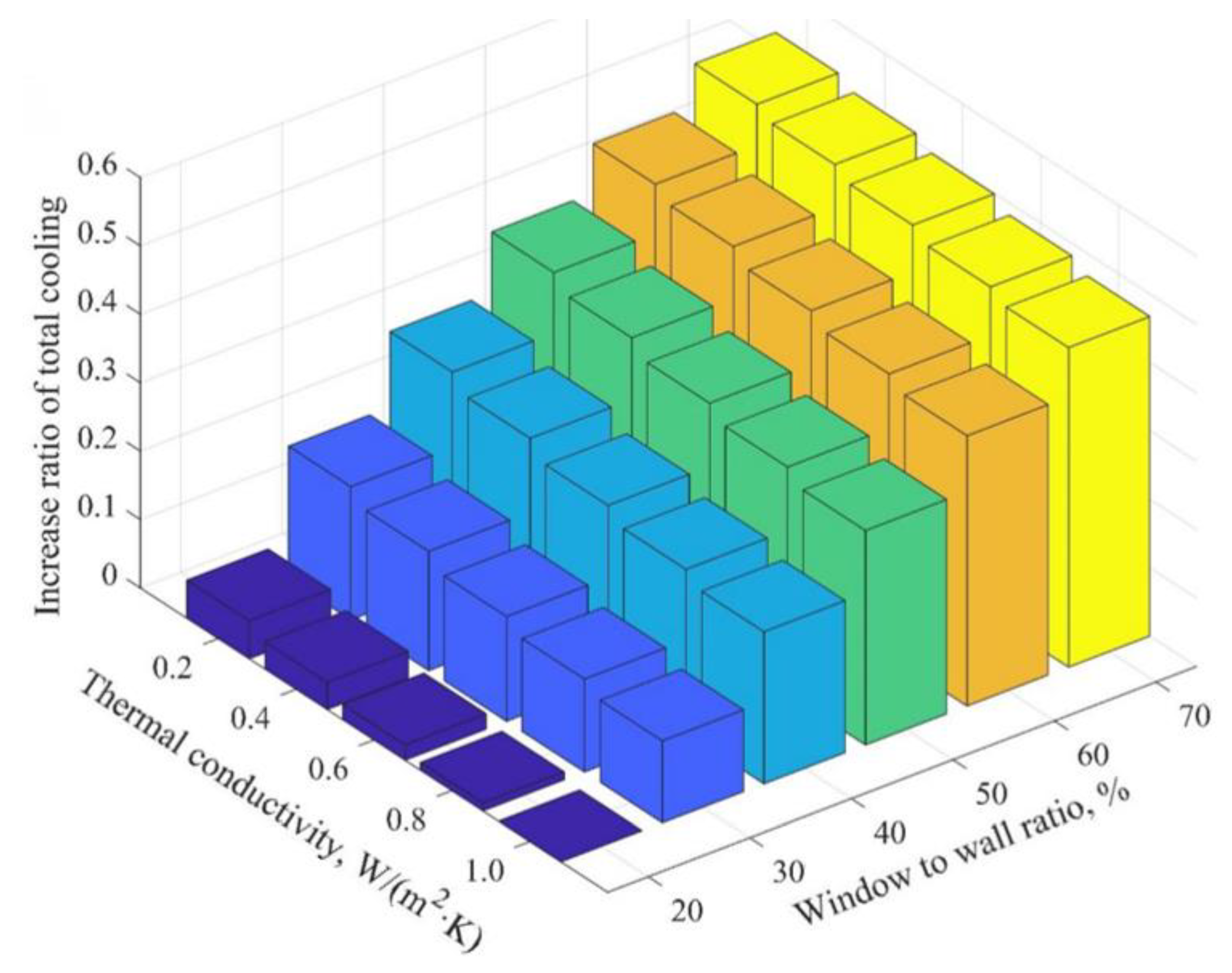
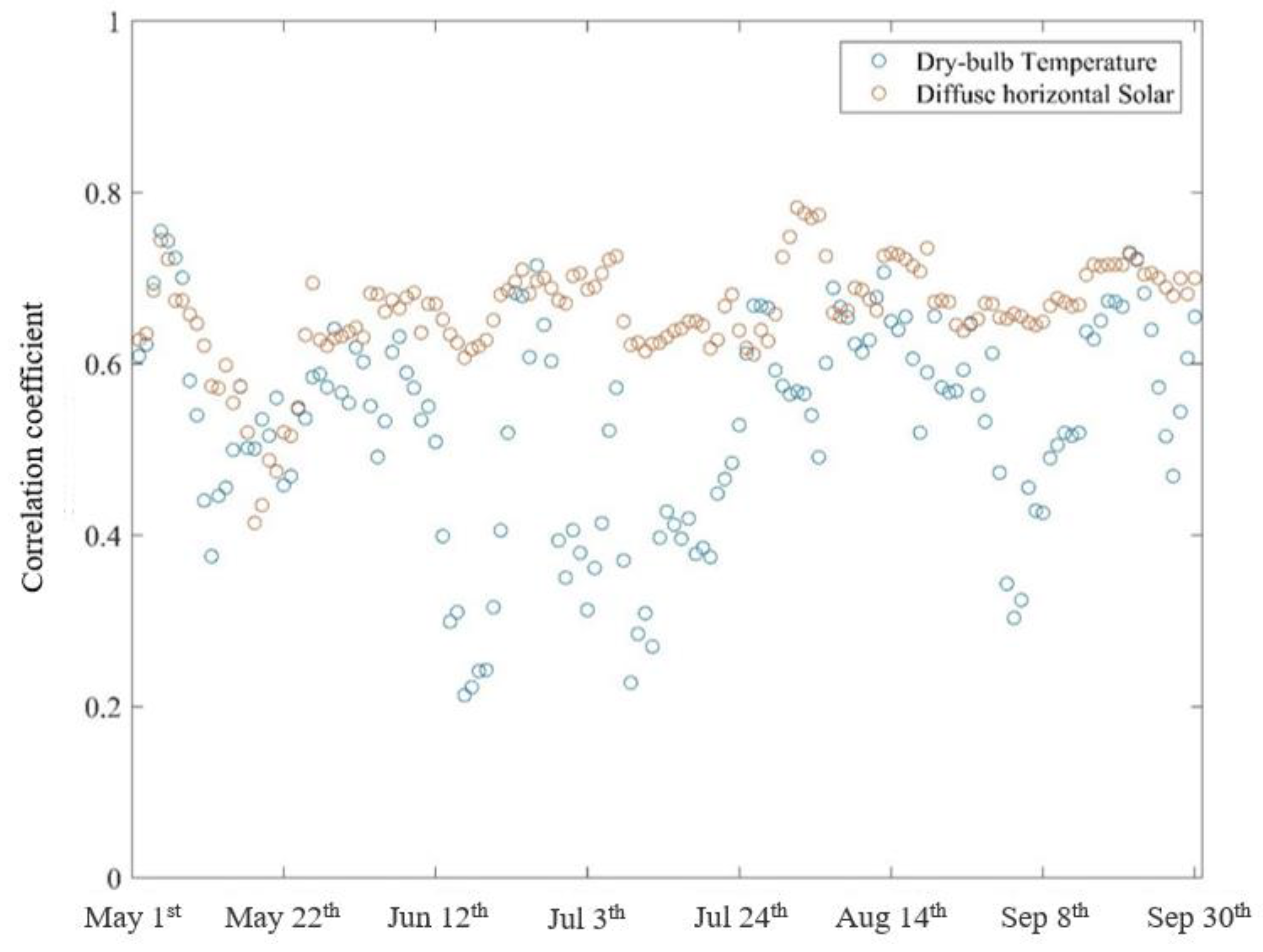
4.1. Analysis of Influencing Factors

The thermal performance and window-to-wall ratio of the building were varied to obtain the air conditioning cooling demand for different situations, as shown in Figure 4. Taking the case with a thermal performance of 1.0 and a window-to-wall ratio of 20% as the baseline, the overall cooling demand for the other cases increases based on the baseline, showing a clear stepwise change trend. Among these, the numerical changes caused by fluctuations in the window-to-wall ratio are more pronounced. The difference between the maximum and minimum values is close to 50%. This gap is partly due to more solar radiation and partly due to the overall decrease in heat transfer performance caused by the increase in windows.

A case study with an external wall heat transfer coefficient of 0.6 and a window-to-wall ratio of 0.5 was selected for correlation analysis. The main influencing factors on air conditioning energy consumption in public buildings were identified through Spearman’s rank correlation coefficient, as shown in Figure 5 below. It is evident that solar radiation is the most significant factor, followed by external air temperature. It is important to note that the external air temperature itself is also significantly influenced by solar radiation. Therefore, further analysis is required to understand the interrelationships among air conditioning energy consumption, external air temperature, and solar radiation. Dry bulb temperature and diffuse horizontal solar radiation were chosen for subsequent analysis.

A refined analysis was conducted using a combination of sliding window and correlation methods. Figure 6 and Figure 7 show the analysis results with sliding window widths of one week and one day, respectively. Overall, the correlation between the two and air conditioning energy consumption is further highlighted through the sliding window approach, generally maintained within the range of 0.4 to 0.8. Additionally, compared to dry bulb temperature, Diffuse Horizontal Solar exhibits a higher correlation. Moreover, as shown in Figure 7, due to the influence of sunrise, sunset, and rainfall, diffuse horizontal solar shows a clear polarization. During the daytime on sunny days, this correlation can exceed 0.8. However, it is zero at other times. This means that, although the impact of irradiance is the most significant, it is not stable and there is a predictable instability in the quantification of flexibility in public building air conditioning systems. Therefore, it is still necessary to study the flexibility of air conditioning from both thermal and light perspectives.

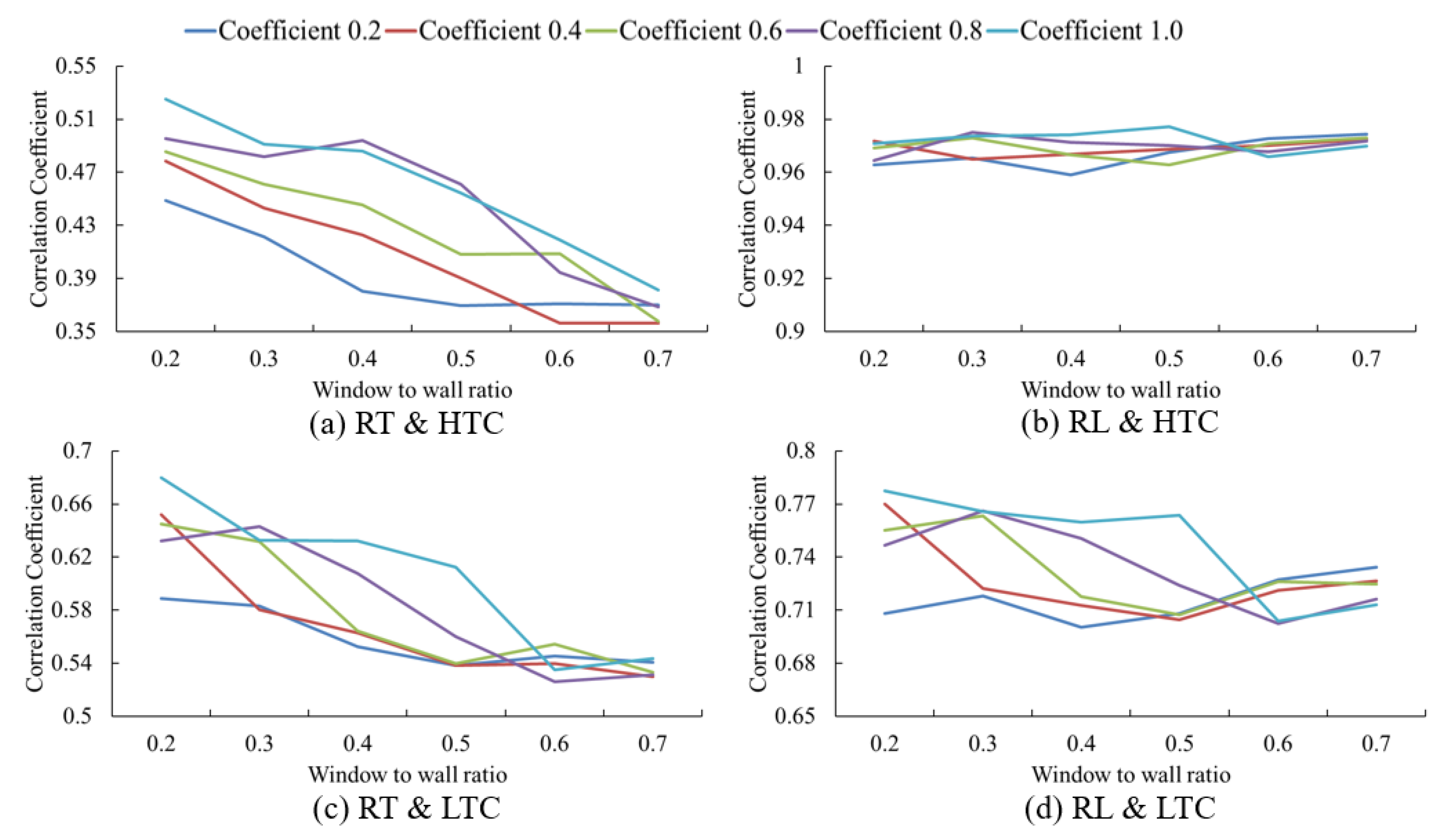
4.2. Similarity Measurement of Light and Heat Transfer Coefficient

Based on different insulation performances and variations in the window-to-wall ratio, changes in the indoor environment were obtained for a scenario in which precooling starts at 8 a.m. and air conditioning is turned off at 10 a.m. to respond to flexible load demands. The response stops when the indoor temperature reaches the upper limit of human comfort (28 °C) and cooling supply resumes. During this process, the corresponding response time (RT) and response energy loss (RL) were recorded. Their correlations with the heat transfer coefficient (HTC) and light transfer coefficient (LTC) are shown in Figure 8. Among them, the correlation between RL and HTC is the highest, exceeding 0.96, indicating that their changes are basically consistent. The correlation between RT and LTC is better compared to HTC but it decreases from 0.7 to 0.5 as the window to wall ratio increases. This indicates that the stability of LTC used for quantitative characterization is flawed. Meanwhile, the correlation between RT and LTC also exceeded 0.7, indicating a certain degree of correlation. The above analysis results regarding correlation are opposite to Figure 6 and Figure 7. Although solar radiation has the highest correlation, a significant portion of its impact overlaps with temperature. When quantitatively characterized, the random fluctuations of solar energy can be amplified, leading to a decrease in effectiveness.

During the correlation analysis process, approximately 20–40% of the data cannot participate in the response scenarios and a large number of zero values may affect the quantification results. This portion of zero values can be filtered using the thermal and light transmission systems. The fitting results obtained after filtering are shown in Figure 9, taking 10:00 as an example. The fitting accuracy is expressed by R² through nonlinear and linear regression analysis. The thermal transmission system shows an exponential correlation with response time, with a fitting degree (R²) of up to 83%. It exhibits a linear correlation with response loss, with a fitting degree of up to 72%. However, the light transmission system does not show any correlation. HTC’s fitting results are also affected by radiation, humidity, and other factors, resulting in errors. Higher irradiance can easily cause rapid loss of cooling in the room. As the indoor temperature increases, the rate of temperature rise gradually decreases. During this process, RT, as a metric parameter for time length, is less affected and is reflected in Figure 9a as having a higher density of data points. RL, as a cumulative energy loss, is easily affected by the initial rapid temperature rise stage, resulting in changes in the total amount, as shown in Figure 9b where the data points are relatively discrete.

The RT and HTC fitting results for 10:00, 12:00, 14:00, and 16:00 are shown in Figure 10. Due to changes in irradiance and temperature, the overall response time shows a decreasing trend over time. At the same time, the fitting degree also decreased. Multiple differences in RT occurred at lower HTC. The main reason may be the difference in sunny or rainy days during the highest irradiation period. This also indirectly indicates that irradiance still has significance in the specific quantification process. Combining the results from Figure 8, Figure 9 and Figure 10, the overall flexibility capability can be characterized in two stages. The first stage involves determining whether flexible adjustment is feasible. The second stage involves assessing the specific energy of the flexible adjustment. In the first stage, the thermal transmission coefficient and light transmission system together construct the building’s flexible adjustability under the coupling of building performance and external environment. For different building envelope structures, window-to-wall ratios, and various time periods, judgments can be made using different coefficients. In the second stage, the thermal transmission coefficient better reflects the impact of the environment on the flexible quantification index, making it necessary to rely more on the thermal transmission coefficient for quantification at the operational level.

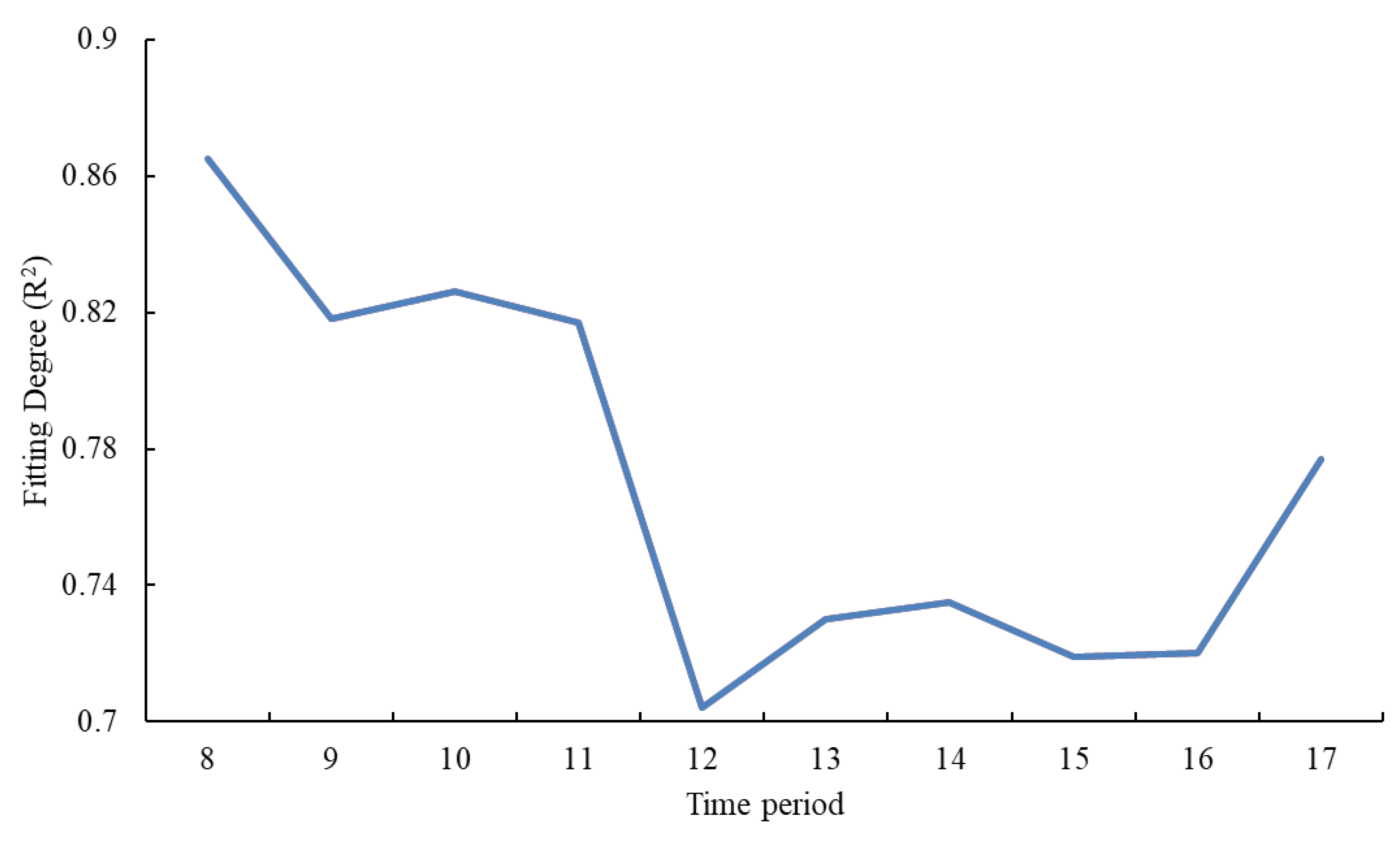
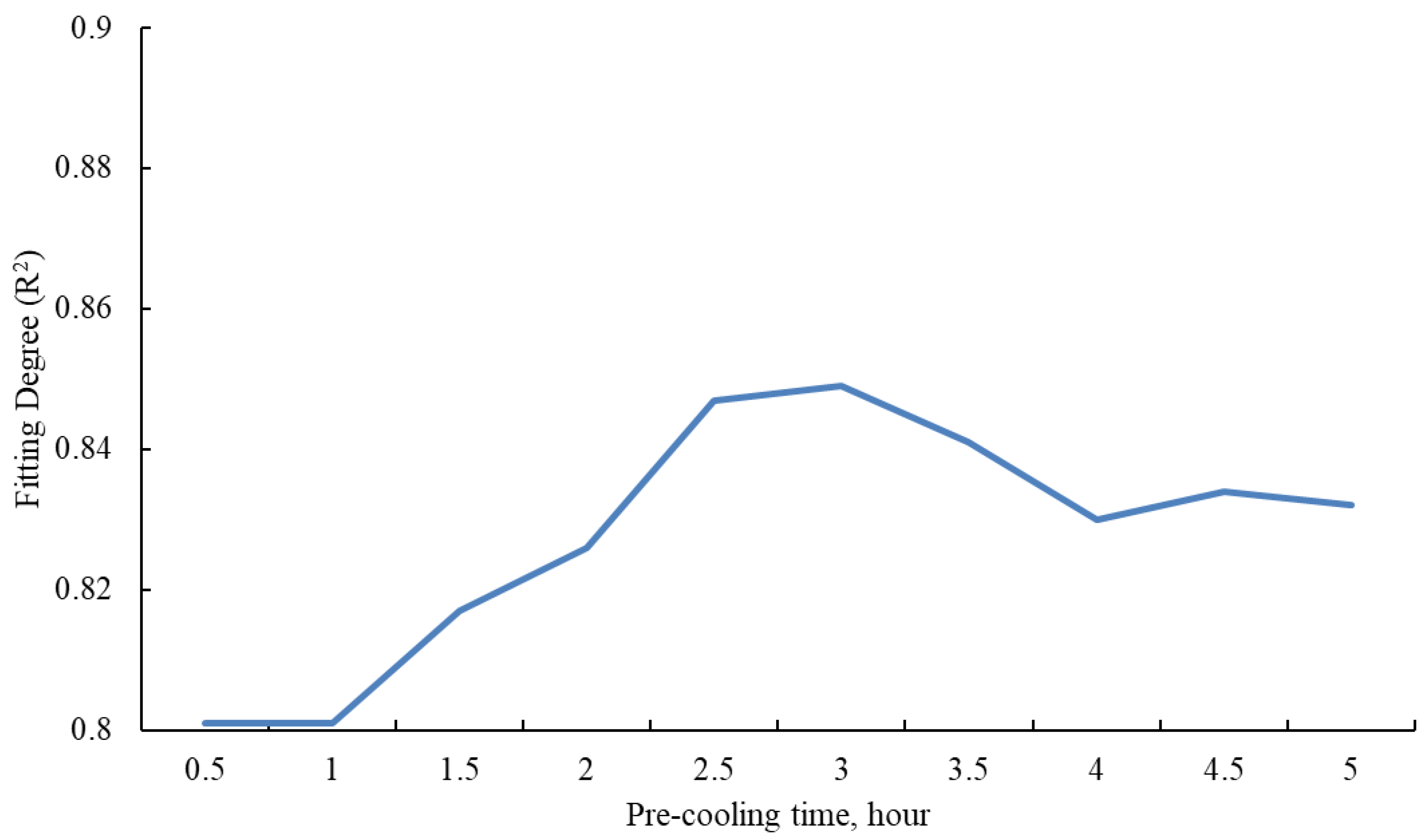
4.3. Analysis of the Influence of Time Period and Precooling Duration

In the previous analysis, both the external environment and the building itself significantly affect flexibility. Therefore, this section selects different time periods to reflect changes in the external environment and different precooling durations to reflect the impact of the building itself. By conducting a sensitivity analysis of the effects of both, the qualitative influence logic of the external environment and the building itself is studied. Figure 11 shows the impact of different time periods on the quantification results. The external temperature and solar irradiation throughout the day both follow a trend of increasing and then decreasing. Therefore, when the response starts at different stages—during the rising phase, the stable phase, and the declining phase—the flexibility capabilities differ significantly. The fitting degree in the morning is relatively high and the fitting degree in the afternoon shows a trend of first decreasing and then increasing. Fortunately, the overall fitting accuracy still exceeds 70%. In addition, the overall trend change also indicates that specific flexible response actions still need to consider the influence of irradiance correction or be combined with masking techniques for collaborative operation [28].

Figure 12 shows the impact of different precooling durations on the quantification results. The fitting accuracy exceeded 80% at the beginning. However, as less precooling time can easily cause rapid temperature rise indoors, a longer precooling time can make indoor temperature changes more stable, resulting in higher fitting accuracy. When the precooling time exceeds 2.5 h, the enhancement effect on response duration significantly diminishes and this can lead to an increase in response loss. Therefore, in different cases, there exists an optimal precooling time that maximizes the balance between benefits and costs, which typically falls within the range of 1 to 2.5 h. This result can also serve as a quantitative reference for the power grid to issue preregulation response instructions.

5. Conclusions

This study proposes a method to express changes in the external environment and intrinsic performance of buildings using unified data through thermal transmission coefficients and light transmission systems, aiming to quantify the flexible adjustability of air conditioning in public buildings. Using an actual case of a public building in Shanghai, differentiated cases with varying insulation performances and window-to-wall ratios were generated through three-dimensional modeling and simulation. Subsequently, factors influencing air conditioning energy consumption were analyzed using sliding window and correlation coupling methods. Then, the application effect of the proposed transmission system in the process of quantifying air conditioning flexibility was studied through fitting analysis. Finally, sensitivity analysis was extended, leading to the following conclusions:

(1)

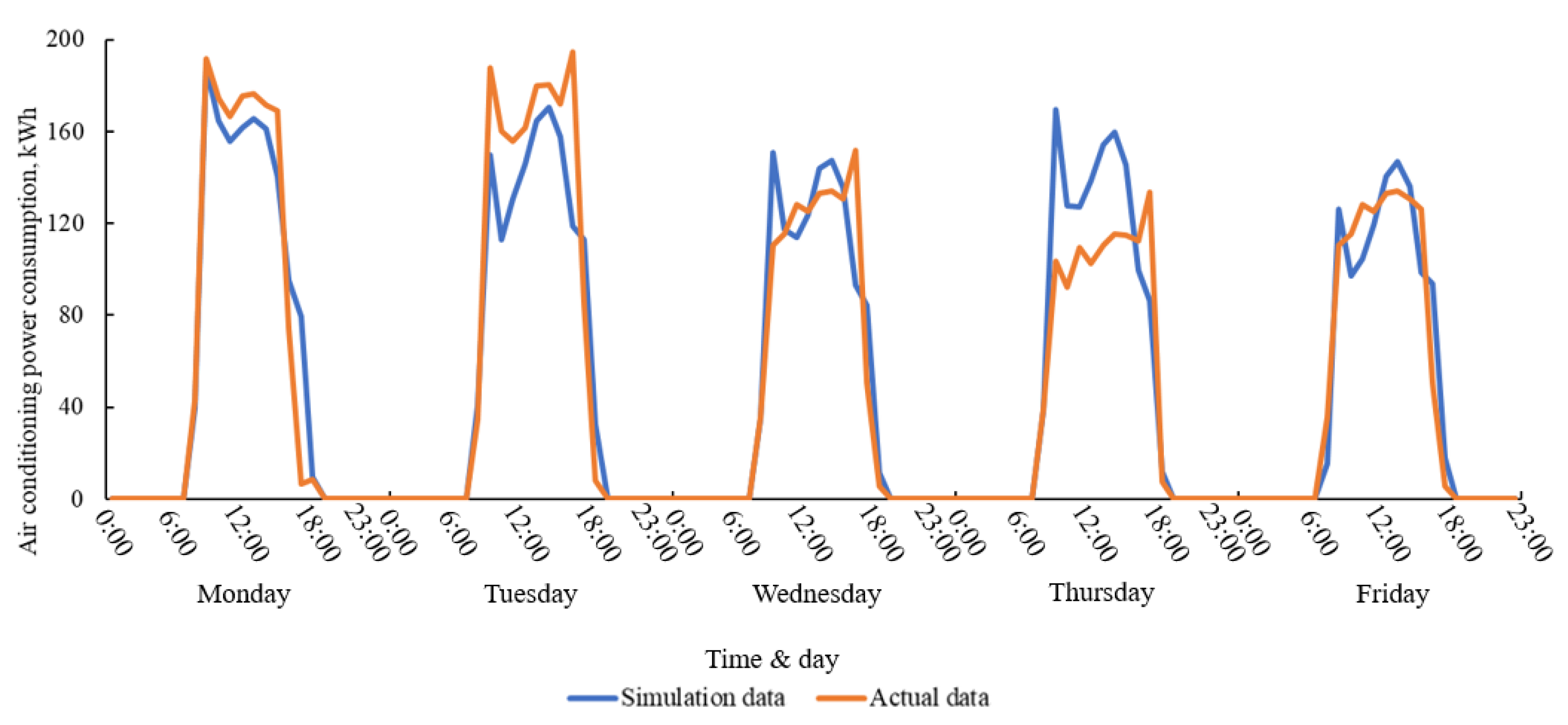
Solar irradiance has the highest correlation but, due to weather and time factors, it exhibits significant variability. This characteristic makes it difficult to achieve a high fitting degree for the light transmission coefficient during the quantification of air conditioning flexibility. Therefore, by comprehensively considering the thermal transmission systems of various enclosure structures, a fitting degree of about 80% can be achieved during the specific quantification stage.

(2)

In the assessment of RT, LTC has a higher correlation than HTC. Therefore, the quantification of air conditioning flexibility response capability can be divided into two stages. The first stage involves a preliminary judgment of whether a response is possible by combining the thermal and light transmission systems. The second stage then involves specific quantification using the thermal transmission system.

(3)

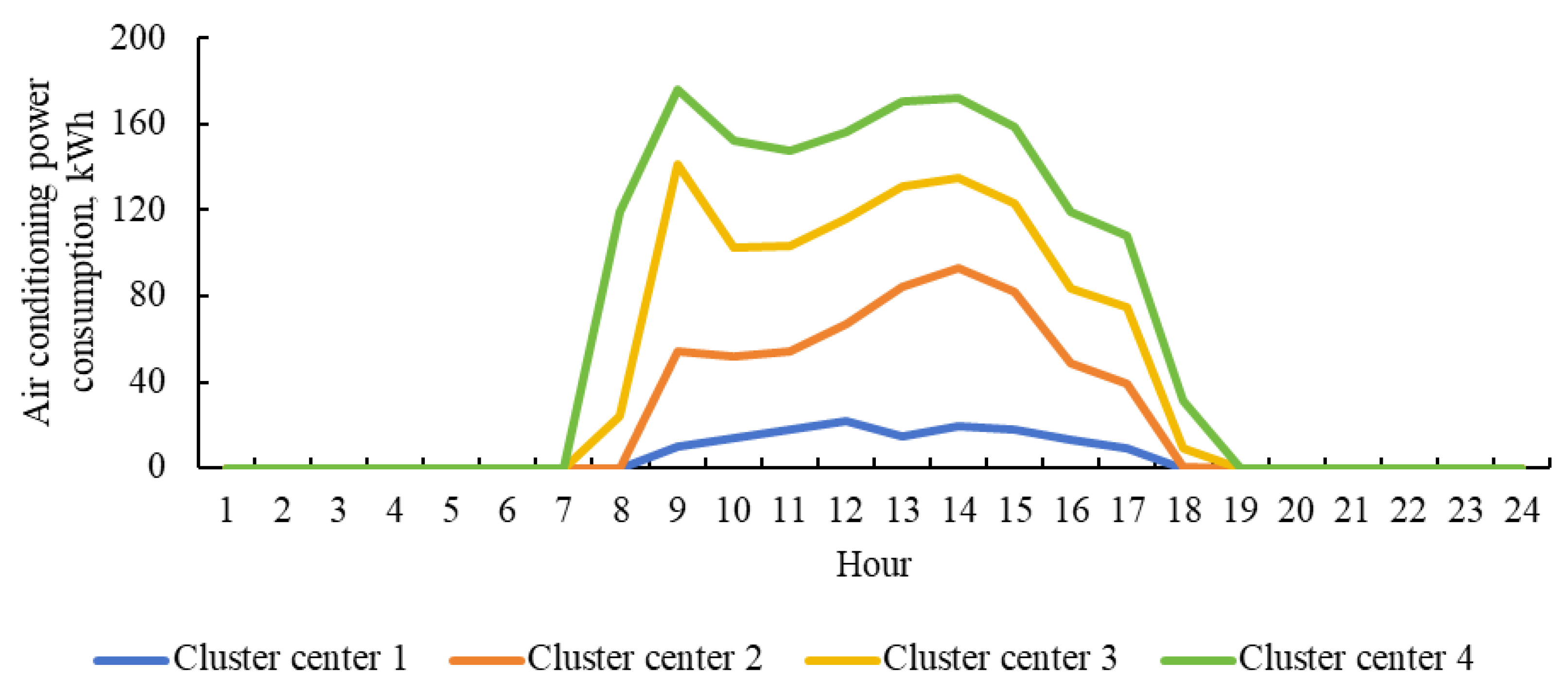
Affected by the external environment, the flexibility regulation capability of air conditioning is greatest during the declining phase in the morning but the grid response demand is relatively low at this time. During the peak grid response demand periods in the afternoon, the flexibility regulation capability of air conditioning is comparatively lower but it can still maintain a fitting degree of over 70%.

This study is derived from an evidence-based simulation analysis of actual cases and can provide quantitative references for the quantification of flexible adjustment capabilities and response participation studies in public building air conditioning. However, the conclusion of this study comes from the analysis of simulation data and there may be more disturbances in practical application scenarios, which may further reduce the accuracy of quantitative representation. Meanwhile, the prediction method used in this study is relatively conventional and there is still room for further improvement in fitting accuracy (for example, deep neural networks, etc.).

At the same time, breakthroughs in technologies such as smart glass and PCM have transformed the fence structure of buildings from static insulation to dynamic energy regulation. This change further enhances the potential for flexible adjustment of air conditioning. PCM can indirectly increase the upper limit of air conditioning cooling capacity. The control of smart glass can reduce the impact of irradiance, thereby further improving the fit between HTC and flexible response indicators.

References

1. Critz, D.K.; Busche, S.; Connors, S. Power systems balancing with high penetration renewables: The potential of demand response in Hawaii. Energy Convers. Manag. 2013, 76, 609–619. [Google Scholar] [CrossRef]
2. Alimohammadisagvand, B.; Jokisalo, J.; Kilpeläinen, S.; Ali, M.; Sirén, K. Cost-optimal thermal energy storage system for a residential building with heat pump heating and demand response control. Appl. Energy 2016, 174, 275–287. [Google Scholar] [CrossRef]
3. Liu, Q.; Li, Y.; Xu, T.; Qian, F.; Meng, H.; Yao, Y.; Ruan, Y. Peak shaving potential and its economic feasibility analysis of V2B mode. J. Build. Eng. 2024, 90, 109271. [Google Scholar] [CrossRef]
4. Salpakari, J.; Lund, P. Optimal and rule-based control strategies for energy flexibility in buildings with PV. Appl. Energy 2016, 161, 425–436. [Google Scholar] [CrossRef]
5. Vellei, M.; Le Dréau, J.; Abdelouadoud, S.Y. Predicting the demand flexibility of wet appliances at national level: The case of France. Energy Build. 2020, 214, 109900. [Google Scholar] [CrossRef]
6. Finck, C.; Li, R.L.; Kramer, R.; Zeiler, W. Quantifying demand flexibility of power-to-heat and thermal energy storage in the control of building heating systems. Appl. Energy 2018, 209, 409–425. [Google Scholar] [CrossRef]
7. Johra, H.; Heiselberg, P.; Le Dreau, J. Influence of envelope, structural thermal mass and indoor content on the building heating energy flexibility. Energy Build. 2019, 183, 325–339. [Google Scholar] [CrossRef]
8. Hurtado, L.A.; Rhodes, J.D.; Nguyen, P.H.; Kamphuis, I.G.; Webber, M.E. Quantifying demand flexibility based on structural thermal storage and comfort management of non-residential buildings: A comparison between hot and cold climate zones. Appl. Energy 2017, 195, 1047–1054. [Google Scholar] [CrossRef]
9. Foteinaki, K.; Li, R.L.; Heller, A.; Rode, C. Heating system energy flexibility of low-energy residential buildings. Energy Build. 2018, 180, 95–108. [Google Scholar] [CrossRef]
10. Lu, F.; Yu, Z.Y.; Zou, Y.; Yang, X. Cooling system energy flexibility of a nearly zero-energy office building using building thermal mass: Potential evaluation and parametric analysis. Energy Build. 2021, 236, 110763. [Google Scholar] [CrossRef]
11. Liu, M.Z.; Heiselberg, P. Energy flexibility of a nearly zero-energy building with weather predictive control on a convective building energy system and evaluated with different metrics. Appl. Energy 2019, 233, 764–775. [Google Scholar] [CrossRef]
12. Ruan, Y.J.; Ma, J.C.; Meng, H.; Qian, F.; Xu, T.; Yao, J. Potential quantification and impact factors analysis of energy flexibility in residential buildings with preheating control strategies. J. Build. Eng. 2023, 78, 107657. [Google Scholar] [CrossRef]
13. Li, Y. The Smart Thermostat of HVAC Systems Based on PMV-PPD Model for Energy Efficiency and Demand Response. In Proceedings of the 2nd IEEE Conference on Energy Internet and Energy System Integration (EI2), Beijing, China, 20–22 October 2018. [Google Scholar]
14. Reynders, G.; Diriken, J.; Saelens, D. Generic characterization method for energy flexibility: Application to structural thermal storage in Belgian residential buildings. Appl. Energy 2017, 198, 192–202. [Google Scholar] [CrossRef]
15. Jensen, S.Ø.; Marszal-Pomianowska, A.; Lollini, R.; Pasut, W.; Knotzer, A.; Engelmann, P.; Stafford, A.; Reynders, G. IEA EBC Annex 67 Energy Flexible Buildings. Energy Build. 2017, 155, 25–34. [Google Scholar] [CrossRef]
16. Arteconia, A.; Mugnini, A.; Polonara, F. Energy flexible buildings: A methodology for rating the flexibility performance of buildings with electric heating and cooling systems. Appl. Energy 2019, 251, 113387. [Google Scholar] [CrossRef]
17. Dréau, J.L.; Heiselberg, P. Energy flexibility of residential buildings using short term heat storage in the thermal mass. Energy 2016, 111, 991–1002. [Google Scholar] [CrossRef]
18. Hu, M.; Xiao, F.; Wang, L. Investigation of demand response potentials of residential air conditioners in smart grids using grey-box room thermal model. Appl. Energy 2017, 207, 324–335. [Google Scholar] [CrossRef]
19. Zhang, W.; Lian, J.; Chang, C.Y.; Kalsi, K. Aggregated modeling and control of air conditioning loads for demand response. IEEE Trans. Power Syst. 2013, 28, 4655–4664. [Google Scholar] [CrossRef]
20. Antonopoulos, I.; Robu, V.; Couraud, B.; Kirli, D.; Norbu, S.; Kiprakis, A.; Flynn, D.; Elizondo-Gonzalez, S.; Wattam, S. Artificial intelligence and machine learning approaches to energy demand-side response: A systematic review. Renew. Sustain. Energy Rev. 2020, 130, 109899. [Google Scholar] [CrossRef]
21. Hongyan, M.; Wang, H.; Yan, Z.; Yu, Q. Evaluating peak-regulation capability for power grid with various energy resources in Chinese urban regions via a pragmatic visualization method. Sustain. Cities Soc. 2022, 80, 103749. [Google Scholar]
22. Ungureanu, S.; Topa, V.; Cziker, A.C. Analysis for non-residential short-term load forecasting using machine learning and statistical methods with financial impact on the power market. Energies 2021, 14, 6966. [Google Scholar] [CrossRef]
23. Yang, X.; Zhang, L.; Zhao, H.; Zhang, W.; Long, C.; Wu, G.; Zhao, J.; Shen, X.; Cao, M. Multi-Level Decomposition and Interpretability-Enhanced Air Conditioning Load Forecasting Study. Energies 2024, 17, 5881. [Google Scholar] [CrossRef]
24. Lian, H.; Wei, H.; Wang, X.; Chen, F.; Ji, Y.; Xie, J. Research on Real-Time Energy Consumption Prediction Method and Characteristics of Office Buildings Integrating Occupancy and Meteorological Data. Buildings 2025, 15, 404. [Google Scholar] [CrossRef]
25. Ma, D.; Sun, Y.; Ma, S.; Ma, H. Energy consumption characteristics and evaluation of public buildings in Tianjin, China. Energy Built Environ. 2024. [Google Scholar] [CrossRef]
26. Huang, H.; Liao, F.; Liu, Z.; Cao, S.; Zhang, C.; Yao, P. Peak Assessment and Driving Factor Analysis of Residential Building Carbon Emissions in China’s Urban Agglomerations. Buildings 2025, 15, 333. [Google Scholar] [CrossRef]
27. Hong, Y.; Ezeh, C.I.; Deng, W.; Hong, S.-H.; Peng, Z.; Tang, Y. Correlation between building characteristics and associated energy consumption: Prototyping low-rise office buildings in Shanghai. Energy Build. 2020, 217, 109959. [Google Scholar] [CrossRef]
28. Lu, S.; Liang, B.; Li, X.; Kong, X.; Jia, W.; Wang, L. Performance Analysis of PCM Ceiling Coupling with Earth-Air Heat Exchanger for Building Cooling. Materials 2020, 13, 2890. [Google Scholar] [CrossRef]
Figure 1. 3D graphs of the research building in simulation software.
Energies 18 01311 g001
Figure 2. Comparison chart between actual data and simulation data.
Energies 18 01311 g002
Figure 3. Typical daily clustering results of simulation data.
Energies 18 01311 g003
Figure 4. Joint influence analysis of thermal conductivity and window to wall ratio.
Energies 18 01311 g004
Figure 5. Overall correlation analysis of influencing factors.
Energies 18 01311 g005
Figure 6. Sliding window and correlation analysis (with a one-week interval).
Energies 18 01311 g006
Figure 7. Sliding window and correlation analysis (with a one-day interval).
Energies 18 01311 g007
Figure 8. Flexibility correlation between different external wall heat transfer coefficient (legend) and window-to-wall ratio (response starting from 10:00).
Energies 18 01311 g008
Figure 9. Quantitative characterization of the flexible response time period (10:00).
Energies 18 01311 g009
Figure 10. Quantitative characterization of RT and HTC.
Energies 18 01311 g010
Figure 11. The influence of different time periods on quantitative characterization results.
Energies 18 01311 g011
Figure 12. The influence of different precooling time on the quantitative characterization results.
Energies 18 01311 g012