Techno-Economic Feasibility and Optimal Design Approach of Grid-Connected Hybrid Power Generation Systems for Electric Vehicle Battery Swapping Station

Abstract

Fossil fuel depletion, environmental concerns, and energy efficiency initiatives drive the rapid growth in the use of electric vehicles. However, lengthy battery charging times significantly hinder their widespread use. One proposed solution is implementing battery swapping stations, where depleted electric vehicle batteries are quickly exchanged for fully charged ones in a short time. This paper evaluates the techno-economic feasibility and optimal design of a grid-connected hybrid wind–photovoltaic power system for electric vehicle battery swapping stations. The aim is to evaluate the viability of this hybrid power supply system as an alternative energy source, focusing on its cost-effectiveness. An optimal control model is developed to minimize the total life cycle cost of the proposed system while reducing the reliance on the utility grid and maximizing system reliability, measured by loss of power supply probability. This model is solved using mixed-integer linear programming to determine key decision variables such as the power drawn from the utility grid and the number of wind turbines and solar photovoltaic panels. A case study validates the effectiveness of this approach. The simulation results indicate that the optimal configuration comprises 64 wind turbines and 402 solar panels, with a total life cycle cost of ZAR 1,963,520.12. These results lead to an estimated energy cost savings of 41.58%. A life cycle cost analysis, incorporating initial investment, maintenance, and operational expenses, estimates a payback period of 5 years and 6 months. These findings confirm that the proposed hybrid power supply system is technically and economically viable for electric vehicle battery swapping stations.

1. Introduction

The growing concerns over climate change, the urgent need to decrease dependence on fossil fuels, and the imperative to mitigate environmental impacts related to energy have spurred global efforts toward transitioning to sustainable energy sources [1,2]. The energy consumption forecast for the coming years further reinforces this pattern, particularly considering the population dynamics and economic development in various countries worldwide [3]. This is highly critical for countries listed as developed countries, where the stakes are high in balancing economic growth with environmental sustainability [2,3]. For instance, in South Africa, the energy sector grapples with multiple challenges, including supply constraints, frequent power outages (load shedding), rising electricity costs, and environmental degradation [4,5]. As part of South Africa’s commitment to sustainable development and energy security, increasing focus is being placed on diversifying the energy portfolio and promoting the adoption of renewable sources.

The adoption of electric vehicles (EVs) has the potential to lower fossil fuel consumption, thereby reducing greenhouse gas (GHG) emissions and other pollutants released into the atmosphere during road transportation. Aside from reducing fossil fuel dependence, EVs emit considerably less carbon dioxide (CO₂) than internal combustion engines (ICEs) [6,7]. With the growing adoption of EVs, the demand for charging infrastructure is steadily rising. Thus, the success of the EV market is closely tied to the availability, efficiency, and accessibility of charging systems [8]. Despite the increasing availability of charging infrastructure, charging times often remain excessively long. This situation necessitates using fast charging methods, which can negatively impact the longevity of EV batteries. A promising approach to addressing these challenges is the implementation of EV battery swapping stations (BSSs).

BSSs offer a more convenient and efficient solution for recharging depleted EV batteries by enabling drivers to swap depleted batteries with fully charged ones in just a few minutes. These stations charge the depleted EV batteries according to a predetermined strategy before making them available for the next swap, effectively alleviating concerns about energy availability and long charging times. BSSs can also charge the depleted EV batteries ahead of time, especially during off-peak hours, to meet the swapping demands. This strategy aligns well with the peak demand periods of the power supply system. The depleted EV batteries being charged can be incorporated into energy management systems. These systems can coordinate their charging cycles or utilize their discharge capacity to supply electricity back to the utility grid [9,10,11,12]. This charging solution is effective for offering seamless mobility since swapping a depleted EV battery takes less time than charging it. Moreover, BSSs can be considered as a demand response resource that benefits both the environment and the power supply system. BSSs are essential in promoting EV adoption and lowering carbon emissions from transportation. Nevertheless, integrating BSSs with the existing power grid remains a significant challenge due to the substantial operating costs related to power generation and system maintenance [13,14,15,16,17,18,19]. These challenges can be addressed by integrating the BSS with renewable energy sources (RESs), which improves grid reliability and supports a more stable power infrastructure.

In light of the growing interest in BSSs, many companies globally are engaging in pilot installations to develop and implement BSS technology for the EV industry, showing that battery swapping technology is a promising and cost-effective alternative to the traditional plug-in charging method [20,21,22,23]. Significant research studies have also focused on developing and optimizing BSSs by integrating them with RESs. These research studies have often investigated different methods to enhance the operation, planning, and management of BSSs, highlighting their potential benefits over the traditional plug-in charging methods. Shalaby et al. introduced a rolling-horizon optimization (RHO) approach for efficiently operating EV BSSs. This framework addresses the limitations of day-ahead models by enabling real-time decision-making for battery swapping and charging. It incorporates a diverse battery inventory and variable-rate chargers to improve grid flexibility. The computational complexity is minimized by transforming a nonlinear problem into an MILP. An extended short-term memory network is used to predict the EV demand. The simulation results show that scheduling based on the RHO framework improves daily profits by 10–25.7% and accommodates 11–14% more EVs than the traditional methods, demonstrating its effectiveness in optimizing resource distribution and meeting demand [24]. Boonraksa et al. examined integrating PV systems with BSSs for electric buses to reduce energy costs and peak demand. The study applies metaheuristic algorithms for optimizing battery charging, with the gray wolf optimizer (GWO) demonstrating the highest efficiency. The results show that GWO-based scheduling lowers the peak demand by 23.43% and cuts the energy costs by 27.63% compared to the conventional methods. This method enhances cost efficiency, grid stability, and operational reliability, highlighting the benefits of metaheuristic optimization in incorporating renewable energy into BSSs [25]. A study by Yan et al. introduced a real-time energy management strategy for a smart community microgrid (SCMG) integrated with BSSs, leveraging variable RESs to simultaneously power EV charging and conventional residential demand. The authors developed a Lyapunov optimization framework grounded in queuing theory, transforming complex energy scheduling into a simplified real-time optimization problem. The simulations demonstrated that dual-purpose BSS operations—serving both EVs and household loads—enhanced the system profitability and RE utilization compared to standalone BSS configurations. This approach highlights the potential of integrated RESs to balance dynamic grid demands while improving economic and sustainability outcomes [26]. Mahoor et al. developed a mathematical model to optimize the operation of BSSs under uncertainty, addressing random customer demand for fully charged batteries and utilizing available batteries to minimize the operational costs through energy reselling and demand shifting. The authors solved the BSS scheduling problem for one station using MILP and predicted battery depletion by presenting a feasible solution. Simulation approaches were also utilized to demonstrate the proposed model’s effectiveness, minimizing its practicality in reaching the lowest possible operating cost [27]. In [28], Liu et al. developed a closed-loop supply chain model for Battery Swapping and Charging Stations (BSCSs) to optimize their combined operation while employing a network-calculus-based service model to ensure quality battery swapping service. Their simulation results demonstrated the model’s effectiveness, showing minimal optimal losses and reduced computational time, confirming its practical applicability. Bian et al. presented an improved uncertainty set for optimizing an Integrated Energy System (IES) with an EV BSS. The proposed framework incorporates N-1 contingency considerations and a source load distribution to enhance the system reliability. A multi-time-scale robust optimization model was developed to minimize the total costs while addressing operational uncertainties. The solution utilizes the nested column and constraint generation algorithm for efficient scheduling. The simulation results confirmed that the method reduces conservatism in uncertainty modeling, ensuring economic efficiency and system stability while meeting EV user demands [29]. Jordehi et al. investigated the optimal placement of battery-swapping stations (BSSs) within a microgrid (MG) that includes micro-pumped hydro storage (PHS), photovoltaic, wind, and geothermal units. Their study considers reactive power dispatch and network constraints using AC optimal power flow while assessing the impact of BSS capacity, charging/discharging limits, and PHS characteristics on the MG performance. The optimization problem is solved using the DICOPT solver in GAMS [30].

Based on cost minimization, Ren et al. proposed a battery energy management platform for charging and swapping applications, integrating hardware design, dynamic load balancing, and hierarchical coordination control for micro-sources. Their approach also includes emergency response strategies to improve system reliability and efficiency. The experimental results demonstrated the platform’s effectiveness in energy scheduling, battery balance, mode switching, and fault protection [31]. Wu et al. developed an optimal charging strategy for PV-based BSSs to enhance the self-consumption of solar energy and service availability while addressing forecast uncertainties. Using PSO, they calculated the optimal charging power for each time slot to minimize costs and improve operational efficiency. The results indicated that the suggested approach significantly minimizes charging costs while enhancing solar energy utilization [32]. Gull et al. proposed an optimal BSS operation using a multi-objective optimization approach that integrates grid power, solar PV, and biogas generation with battery arrivals. The strategy, implemented through MILP and time-dependent dynamic programming, reduces charging costs and enhances revenue by enabling battery-to-grid operation. The results show that this approach increases the daily net profit significantly, demonstrating its potential to improve the financial viability and adoption of BSSs in the EV market [33]. In [34], Fachrizal et al. introduced an optimal sizing framework for workplace solar-powered EV charging stations, utilizing a novel self-consumption–sufficiency balance (SCSB) metric to balance energy self-consumption (SC) and self-sufficiency (SS). Their findings indicated that larger PV-EV systems yield higher SCSB scores, while innovative charging strategies improved SC and SS by up to 42.6 and 40.8 percentage points, respectively. The study proposes the SCSB-based framework as a universal benchmark for optimizing distributed generation–load systems due to its simplicity and adaptability [34].

Previous research has focused on optimizing BSSs by exploring various strategies and approaches to improve efficiency, such as optimal location and sizing of stations, dynamic scheduling and dispatching of EV batteries, and incorporating renewable energy to reduce the carbon footprint and operational costs. However, these studies overlook a detailed assessment of the technical feasibility and cost-effectiveness of incorporating RESs (e.g., solar and wind) alongside smart grid solutions. Such integrations could improve the efficiency and sustainability of battery-swapping networks in grid-connected hybrid systems, even without a dedicated battery energy storage infrastructure.

To the best of the authors’ knowledge, no prior studies have investigated the application of grid-connected hybrid renewable energy systems to EV BSSs within the South African context. This gap in the literature motivated the current study. The rapid increase in EV adoption, influenced by new vehicle brands, infrastructure development, and government initiatives aimed at reducing transport sector emissions by 5% by 2050, underscores the need for cleaner mobility solutions in South Africa [35,36,37]. Although the number of public EV charging stations continues to expand nationwide, insufficient infrastructure remains a significant obstacle to the broader adoption of EVs [37,38]. Effective BSS design and operation must address complex factors, including the intermittent nature of RE, EV battery charging patterns, EV battery swapping demand, and utility grid stability. This paper investigates the techno-economic feasibility and optimal design of grid-connected hybrid power generation systems to support EV BSSs, thereby filling the gap. A multi-objective optimization model is formulated to minimize the total LCC $\left(LC{C}_{Tot}\right)$ of the proposed system and the electricity cost incurred from the utility grid $\left(C_{Eg}\right)$ while simultaneously maximizing system reliability, represented by the loss of power supply probability (LPSP). This developed multi-objective optimization model can provide the EV BSS with a continuous power supply at a low cost, and the scheduling strategy can be implemented for the swapping EV battery so that the swapping demand must be satisfied at any given time of the day. Understanding these aspects is essential for maximizing benefits and ensuring the sustainability of EV BSSs. Therefore, mixed-integer linear programming (MILP) is employed for multi-objective optimal sizing, offering advantages over heuristic algorithms due to the quick solvability of linear programming (LP) sub-problems and the guarantee of obtaining the global optimum through a convex feasible region [39].

The subsequent sections of the paper are organized as follows: Section 2 defines the mathematical model formulation, including the technical and economic parameters. Section 3 displays the general data reflecting the real-world operational conditions. The simulation results and discussion are presented in Section 4. Lastly, Section 5 concludes the paper.

2. Mathematical Model Formulation

A mathematical model has been developed to evaluate the feasibility and performance of the proposed hybrid power supply system for an EV BSS. This model aims to optimize system operation by minimizing the total life cycle cost while ensuring a reliable power supply. The formulation incorporates key decision variables, including grid power consumption, the number of WTs, and the number of solar PV panels. Constraints related to power balance, system reliability, and economic feasibility are considered. The optimization problem is solved using mixed-integer linear programming, ensuring an efficient allocation of resources and cost-effective system operation.

2.1. Schematic Model Layout

Figure 1 illustrates the schematic layout of the proposed grid-connected wind–photovoltaic hybrid power generation system designed for the EV BSS. The main components of the proposed system are the vertical wind turbines (WTs), the solar photovoltaic generator (PV), the inverters, and the battery swapping station (BSS), which comprises the charging apparatus and swapping service for the depleted EV batteries. For such a proposed system, the size of the hybrid renewable power generation system depends on the charging and swapping demand service at the BSS. The BSS uses three distinct sources of electrical energy to recharge the depleted swapped EV batteries. These sources include the electricity generated by vertical WT, the electricity generated by the solar PV generator, and the electricity acquired from the utility grid. To ensure that the demand for swapping depleted EV batteries is met efficiently, it is crucial to accurately determine the properties of power sources utilized to charge the depleted EV batteries. By doing so, the charging process can be optimized to effectively replenish the EV batteries and meet the needs of the drivers. The depleted EV batteries are charged with the utmost priority using clean and renewable energy generated by the vertical WT and solar PV generator. This ensures optimal charging of depleted EV batteries while minimizing electricity use from the utility grid. However, the charging process depends on the accessibility of sufficient resources. In other words, if the electricity generated by the vertical WT and solar PV generator is inadequate, the utility grid supplies the necessary power to charge the depleted EV batteries. Suppose the electricity generated by the vertical WT and solar PV generator exceeds the charging demand of the depleted EV batteries. In that case, the excess electricity can be sold back to the utility grid. The fluctuating electricity prices throughout the day significantly influence the overall cost of the charging process. Implementing a time-of-use (TOU) tariff helps to manage this cost by strategically selecting the power source for recharging depleted EV batteries. The TOU tariff is strategically designed to incentivize power consumption during off-peak periods when electricity prices are at their lowest. This approach serves the dual purpose of minimizing stress on the utility grid during peak hours and optimizing the cost-effectiveness of the charging process. Depending on the prevailing TOU tariffs, the BSS can be supplied by either hybrid power generation or the utility grid. This flexibility enables the BSS to draw power from the utility grid during off-peak periods, leading to cost savings. By doing so, the power flow from the utility grid is managed efficiently and cost-effectively, maintaining reliability and stability. This strategic utilization of the TOU tariff and power source selection not only minimizes operational costs but also contributes to the overall sustainability and resilience of the EV charging infrastructure. The decision to charge the depleted EV batteries is determined by multiple factors, such as the power flow’s limitations and the TOU electricity tariff within the utility grid. The power flow’s limitations depend on the available power capacity and the current power demand in the system. The TOU tariff considers the cost of electricity at different times of the day, where charging the depleted EV batteries during off-peak periods can be more cost-effective. On the other hand, the decision to replace the depleted EV batteries with fully charged ones is determined by the EV driver’s arrival or the swapping service demand at the BSS. The BSS can offer a convenient solution for EV drivers who want to continue their journey without waiting for their EV battery to charge. In this paper, the electrical energy generated by the renewable hybrid power generation system is deliberately not reintegrated into the utility grid.

2.2. Sub-Models of the Proposed System Components

The subsequent sections present detailed descriptions and mathematical models of each component within the proposed hybrid power system.

2.2.1. Wind Turbine System

In wind energy systems, the air is moved to generate power through its kinetic energy. Wind energy is a resource that has the potential to be abundant and that might be easily harvested and converted into useful energy using standard technology. In addition to enabling the efficient utilization of distributed resources, wind energy systems promise to make energy supply systems more flexible, robust, secure, stable, and profitable [40]. As a result, it is crucial to have a reliable assessment of the resources available at a wind farm to generate electricity there. In general, when the wind speed ranges between the “cut-in wind speed” ($V_{ci}$) and the “rated wind speed” $\left(V_r\right)$, the power output of the WT is proportional to the cube of the wind speed. The model used to determine the power output of the WT is displayed in Figure 2. When the wind speed is below the cut-in speed, the WT is unable to generate electricity. Once the wind speed surpasses the cut-in speed, the power generated by the WT increases with the cube of the wind speed, reaching its maximum output at the rated speed. It is known as the rated power $\left(P{r}_{WT}\right)$, and it is the power for which the wind turbine is designed. As shown in Figure 2, the wind speed is very high at some given time, which is dangerous for wind turbines. This is referred to as “cut-out wind speed” $\left(V_{co}\right)$. The wind turbine operation must stop at this point because it has reached the $\left(V_{co}\right)$. Equation (1) represents a description of the simplest straightforward model of this behavior to simulate the power output of the WT [41]:

$$p_{WT}\left(t\right)=\left\{\begin{array}{ll}0& V\left(t\right)\le V_{ci}\\ P{r}_{WT}{\displaystyle \frac{V\left(t\right)-V_{ci}}{V_r-V_{ci}}}\hfill & V_{ci}\le V\left(t\right)\le V_r\\ P{r}_{WT}\hfill & V_r\le V\left(t\right)\le V_{co}\\ 0\hfill & V\left(t\right)\ge V_{co}\end{array}\right.$$

(1)

where $V\left(t\right)$ denotes the wind speed at sampling time t, $V_r$ denotes the rated wind speed, $V_{ci}$ denotes the cut-in wind speed, $V_{co}$ denotes the cut-out wind speed, and $P{r}_{WT}$ denotes the rated power of the wind generator. If the wind speeds and rated power are known, Equation (1) can be used to calculate the power output of the WT. Thus, the rated power of the WT generator can be expressed as

$$P{r}_{WT}={\displaystyle \frac{1}{2}}{\eta }_t{\eta }_g{\phi }_a{C}_p{A}_{WT}{V}_r^3$$

(2)

where ${\eta }_t$ denotes the gearbox efficiency, ${\eta }_g$ denotes the generator efficiency, ${\phi }_a$ denotes the density of air, $C_p$ denotes the power coefficient of the WT, which is the ratio of the power output of the wind generator divided by maximum power, and $A_{WT}$ denotes the sweeping area of the turbine rotor. In contrast, $V_r$ denotes the rated wind speed.

Adjustments to the wind speed profile may be required to optimize energy generation from the WT system depending on the turbine’s height. The wind speed profiles can be simulated using two mathematical models: the logarithmic law and the power law. As a standard analytical approach in the field, this paper employs the power-law model to calculate wind speed at the hub height [42]. When applying this model, the wind speed at the hub height is calculated from

$${\displaystyle \frac{V}{V_{ref}}}={\left({\displaystyle \frac{h}{h_{ref}}}\right)}^{\alpha }$$

(3)

where $V_{ref}$ denotes the wind speed measured at the reference height ($h_{ref}$), V denotes the wind speed measured at the hub height (h), and $\alpha$ denotes the coefficient of ground surface friction, which has a value of more than 0.25 in forested areas and less than 0.1 in flat or watery areas [42].

Multiple WTs can be coupled in parallel to meet the proposed system requirements. One of the design variables is the number of WTs ($N_{WT}$) when operating in parallel. The size of the WT is among the variables that influence the power output of the WT. When $N_{WT}$ is taken into account as the number of WTs, the power output generated by the WT at sampling time $\left(t\right)$ is calculated from

$$P_{WT}\left(t\right)=N_{WT} p_{WT}\left(t\right)$$

(4)

Under varying operational conditions, the net power supply of the WT to the power system is limited by boundaries, which can vary between zero and the maximum power output generated. This relationship can be mathematically expressed as

$$0\le P_{WT}\left(t\right)\le P_{WT}^{max}\left(t\right)$$

(5)

where 0 is the minimum capacity of the power output generated by the WT and $P_{WT}^{max}$ is the maximum capacity of the power output generated by the WT.

Furthermore, the limited availability in number of WTs is constrained so that

$$N_{WT}^{min}\le N_{WT}\le N_{WT}^{max}$$

(6)

where $N_{WT}^{min}$ is the minimum number of WTs taken as zero and $N_{WT}^{max}$ is the maximum number of WTs that can fit into the allocated area as provided by

$$N_{WT}^{max}={\displaystyle \frac{A{T}_{WT}}{A_{WT}}}$$

(7)

where $A{T}_{WT}$ is the total sweeping area available for the WT at the EV BSS and $A_{WT}$ is the sweeping area of the WT rotor.

2.2.2. Solar Photovoltaic System

As the name suggests, the principle of the electricity generated by the PV is related to photons and voltage. By definition, PV is a technology that converts the radiant (photon) energy from sunlight into DC power [43]. A PV cell is a crucial element in converting light energy directly into electricity through a chemical and physical process called the PV effect. The term describes a device whose electrical properties change when exposed to light, such as voltage, current, or resistance. Solar PV panels, also known as solar PV modules, comprise solar PV cells. A solar PV module or solar PV panel comprises several solar PV cells arranged in an integrated group, all facing the same direction. In contrast, an array or solar PV array comprises the solar PV module or solar PV panel connected in parallel, series, or a combination of the two [44]. The size of the PV panel, its efficiency, solar radiation, and the surrounding temperature all affect how much electricity the PV system can generate. The power output generated by a solar PV array is provided by [44]

$$p_{PV}={\eta }_{PV}{A}_{PV}{I}_{PV}$$

(8)

where $p_{PV}$ is the power output generated by the PV array, $A_{PV}$ is the area of the PV array exposed to solar radiation, $I_{PV}$ is the solar radiation that reaches the PV array, and ${\eta }_{PV}$ is the energy conversion efficiency of the PV generator.

It is possible to express the solar irradiation according to the time during the day using

$$I_{PV}\left(t\right)=R_B\left[I_B\left(t\right)+I_D\left(t\right)\right]+I_D\left(t\right)$$

(9)

where $R_B$ is a geometric factor used to indicate the ratio between plane-tilted beams’ irradiation incident and plane-horizontal beams’ standard irradiation, $I_D\left(t\right)$ is the diffuse irradiation, and $I_B\left(t\right)$ is the hourly global irradiation.

The ambient temperature and hourly isolation impact the solar PV generator energy conversion efficiency $\eta$. It can be stated that

$${\eta }_{PV}={\eta }_r{\eta }_{pc}\left[1-\beta \left(T_c-T_{c_{ref}}\right)\right]$$

(10)

where $\beta$ denotes the temperature factor for PV generator efficiency, which ranges from 0.004 to 0.006 per °C, $T_{c,ref}$ denotes the reference cell temperature, ${\eta }_{pc}$ denotes the efficiency of power conditioning, $T_c$ denotes the cell temperature, and ${\eta }_r$ denotes the manufacturer-rated efficiency of the solar array module. The cell temperature is

$$T_c=T_a+\left({\displaystyle \frac{T_{NOCT}-20}{800}}\right)I_{PV}\left(t\right)$$

(11)

where $T_{NOCT}$ is the nominal cell operating temperature, while $T_a$ is the ambient temperature.

The power output of a PV array depends on the number of installed PV panels ($N_{PV}$). Factors such as the size of the panels and others influence the total power generated by the PV system. When considering $N_{PV}$ as the number of solar PV panels, the total power output generated by the PV panels at a given sampling time $\left(t\right)$ can be calculated from

$$P_{PV}\left(t\right)=N_{PV} p_{PV}\left(t\right)$$

(12)

Depending on the operation conditions, the net power supply of the solar photovoltaic panels to the power system is determined by sizing and optimal positioning, and it can vary between zero and the maximum power output generated. This can be stated in the following way:

$$0\le P_{PV}\left(t\right)\le P_{PV}^{max}\left(t\right)$$

(13)

where 0 and $P_{PV}^{max}$ represent the minimum and maximum capacity of the solar PV panel, respectively.

Furthermore, the limited availability number of solar PV arrays is constrained so that

$$N_{PV}^{min}\le N_{PV}\le N_{PV}^{max}$$

(14)

where $N_{PV}^{min}$ is the minimum number of solar PV panels taken as zero and $N_{PV}^{max}$ is the maximum number of solar PV panels that can fit into the allocated area as provided by

$$N_{PV}^{max}={\displaystyle \frac{A{T}_{PV}}{A_{PV}}}$$

(15)

where $A{T}_{PV}$ denotes the total available surface area for the solar PV panel at the EV BSS and $A_{PV}$ denotes the area of the PV array that is exposed to solar radiation.

2.2.3. Inverter

The inverter is a very important device in grid-connected renewable energy systems. It is used to synchronize the output power and set the output voltage. Inverters convert DC power sources to AC power and vice versa. The power output of the WT is in AC electricity, which is transformed into DC by the inverter for later use. The charging demand is in AC power form, and the power output from the solar PV system, which is in DC electricity, is converted again by the inverter to AC electricity. The inverters provide other features to ensure the protection and monitoring of power instability for the entire system. Therefore, it is essential to have high inverter efficiency. The inverter efficiency is provided by [45]

$${\eta }_{INV}={\displaystyle \frac{P_{out}\left(t\right)}{P_{in}\left(t\right)}}$$

(16)

where ${\eta }_{INV}$ is the efficiency of the inverter, $P_{out}$ is the power out from the inverter, and $P_{in}$ is the power that enters into the inverter. In order to ensure safe operation and efficiency, the inverter’s rated power should often be oversized by 10% to 30% [46]. Therefore, the inverter-rated power is

$$P{r}_{INV}=\sum _{t=1}^N{P}_{in}\left(t\right)K_{INV}$$

(17)

where $K_{INV}$ is the oversized coefficient of the inverter. The inverter lifetime is less than the installation lifespan. The total number of inverter replacements required over the system’s operational lifetime can be quantified as

$$N_{Rep,INV}={\displaystyle \frac{L_p}{L_{INV}}}-1,$$

(18)

where $L_p$ is the lifetime of the installation project, while $L_{INV}$ is the lifetime of the inverter.

2.2.4. Utility Grid Power Supply System

The current utility grid was not designed to accommodate the charging demand of depleted EV batteries [47]. In contrast to household loads, the full charge of the depleted EV batteries requires high power levels and substantial amounts of energy [48,49]. Charging the depleted EV batteries can have a significant impact on voltages, component loads, and losses depending on the supplied loads and the design of the utility grid. The impacts on the utility grid are significantly influenced by the charging power and penetration level of the EVs. The number of EV batteries as a percentage of all EVs at the BSS is the general definition of the penetration level. The power from the utility grid is modeled as an all-time available power source for recharging depleted EV batteries at the BSS. The total energy supplied by the utility grid is provided by

$$E_g=\sum _{t=1}^N{P}_{G-BSS}\left(t\right) \Delta t$$

(19)

where $P_{G-CSS}$ is the power flow from the utility grid to charge the depleted EV batteries at the BSS and $\Delta t$ is the sampling time.

Therefore, the energy cost that can be extracted from the utility grid is established by the local electricity market policy and time of use (TOU) tariff. Two parameters are required for utility grid modeling: the utility grid’s maximum power demand (measured in kW), which defines the upper limit of electricity that can be drawn, and the energy procurement cost (expressed in ZAR/kWh), representing the cost of electricity supplied by the utility grid. The energy cost $C_{Eg}$ that can be drawn from the utility grid when charging the depleted EV batteries can be calculated from

$$C_{Eg}=p_e\left(t\right)\sum _{t=1}^N{P}_{G-BSS}\left(t\right) \Delta t$$

(20)

where $P_e\left(t\right)$ is the TOU electricity price at the t-th sampling interval per kWh. Additionally, the power drawn from the utility grid can be constrained to a limited range using

$$0\le P_{G-BSS}\left(t\right)\le +\infty$$

(21)

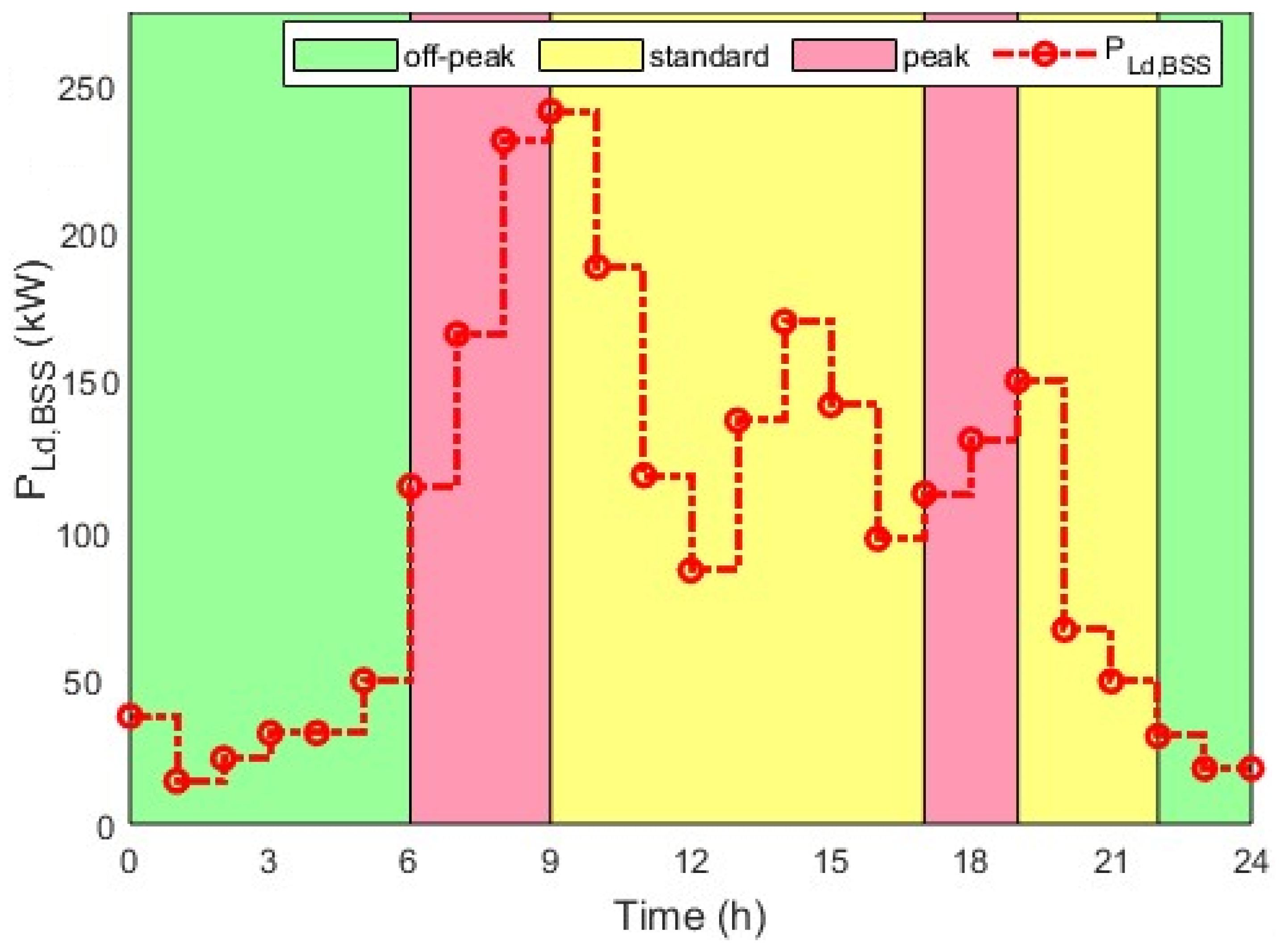
2.2.5. Battery Swapping Station Power Demand Mathematical Modeling

An EV BSS is a facility designed for EV owners to efficiently exchange their depleted EV batteries for fully charged ones in just several minutes. This innovative concept has emerged as a potential solution to address the challenges associated with traditional plug-in charging methods for EVs [22,23]. A standard EV BSS has one or more battery swapping units, enabling multiple EVs to exchange their depleted EV batteries simultaneously. Several factors, such as the charging and swapping processes of depleted EV batteries and the specific characteristics of the EV batteries themselves, typically influence the power demand of a BSS. These specific characteristics encompass parameters such as EV battery capacity, EV battery technology, and the depleted EV battery’s state of charge (SoC) before charging [50]. Proper modeling of power demand at the BSS is crucial, especially during the charging period of depleted EV batteries, to ensure sufficient supply for swapping demand when EVs arrive. Equations (22) and (23), respectively, represent the total charged and discharged power of depleted EV batteries at the BSS. These equations calculate the cumulative power by summing the power contributions or power outputs of all depleted EV batteries present at the BSS [51].

$$P_{c,BSS}\left(t\right)=\sum _{EV,b=1}^n{P}_{c,(EV,b)}\left(t\right)$$

(22)

$$P_{d,BSS}\left(t\right)=\sum _{EV,b=1}^n{P}_{d,(EV,b)}\left(t\right)$$

(23)

where n is the total number of depleted EV batteries at the BSS, $P_{c,BSS}\left(t\right)$ is the total charging power of the depleted EV batteries at the BSS, $P_{d,BSS}\left(t\right)$ is the total discharging power of the depleted EV batteries at the BSS, $P_{c,(EV,b)}\left(t\right)$ is the charging power of one depleted EV battery at the BSS, and $P_{d,(EV,b)}\left(t\right)$ is the discharging power of one depleted EV battery at the BSS. Each depleted EV battery undergoes a charging or discharging process similar to a conventional battery. The charging process of depleted EV batteries is determined by their state of charge (SoC) at specific time intervals, representing the available capacity relative to the maximum capacity when fully charged. Taking these factors into account, the SoC of every EV battery at tth sampling interval inside the BSS can be generally expressed by [27,51]

$$SO{C}_{EV,b}\left(t\right)=SO{C}_{EV,b}(t-1)+\left(P_{c,(EV,b)}\left(t\right)-{\displaystyle \frac{P_{d,(EV,b)}\left(t\right)}{{\eta }_{EV,b}}}\right)\times I_{dur}\left(t\right)$$

(24)

where $I_{dur}\left(t\right)$ is the duration of time interval in minutes and ${\eta }_{EV,b}$ is the efficiency of one EV battery (%) and provided by Equation (25).

$${\eta }_{EV,b}={\displaystyle \frac{{\sum }_{t=1}^N{P}_{d,(EV,b)}\left(t\right)\times I_{dur}\left(t\right)}{{\sum }_{t=1}^N{P}_{c,(EV,b)}\left(t\right)\times I_{dur}\left(t\right)}}$$

(25)

The battery swapping procedure at a BSS involves replacing a depleted EV battery with a fully charged one from an incoming EV. This swap period prevents the EV battery from charging or discharging as the swapping operation progresses. As a result, the EV battery’s power and SoC are reset to zero during the swapping period, as defined by Equation (26).

$$\left\{\begin{array}{cc}{P}_{c,(EV,b)}\left(t\right)=0\hfill & \\ P_{d,(EV,b)}\left(t\right)=0\hfill & \hspace{1em}\forall t=t_{swap}\hfill \\ SO{C}_{EV,b}\left(t\right)=0\hfill & \end{array}\right.$$

(26)

Before the battery swapping period, the depleted EV battery must be fully charged in preparation for the next swap. Thus, the energy management system must guarantee that an adequate number of fully charged EV batteries are available at each time interval to meet the demand for upcoming swaps. This requirement is articulated in Equation (27).

$$SO{C}_{EV,b}\left(t\right)=SO{C}_{EV,b}(t-1)\hspace{1em}\forall t=(t_{swap}-1)$$

(27)

The total power demand at the BSS is based on the power capacity of the charging station. The discretized charging power demand for each depleted EV battery is added together to determine the overall charging power demand. In other words, the total expected power demand required to charge all n depleted EV batteries at the BSS during time t can be calculated using Equation (28).

$$P_{Ld,BSS}\left(t\right)=\sum _{EV,b=1}^n\left(P_{c,(EV,b)}\left(t\right)-P_{d,(EV,b)}\left(t\right)\right)$$

(28)

where $P_{Ld,BSS}\left(t\right)$ is the total expected power demand of all depleted EV batteries charged at time $\left(t\right)$ and n is the total number of depleted EV batteries at the BSS.

2.3. Technical and Economic Parameters of the Proposed System

Before applying the optimization design, it is necessary to define technical and economic parameters to systematically define the proposed system’s total cost and reliability. In this paper, the total life cycle cost $\left(LC{C}_{Tot}\right)$ is used to evaluate the overall system cost, while the loss of power supply probability (LPSP) measures the system’s reliability. The details of these two parameters are explained below.

2.3.1. Economic Evaluation Parameters of the Proposed System

The economic evaluation indicators are mathematical methods used to compare the costs and benefits of the installations in terms of economic, commercial, and social aspects. These indicators play a crucial role in the optimization design of grid-connected hybrid systems [52,53]. This paper considers the economic parameter based on the life cycle cost (LCC) concept as the economic criterion to evaluate the financial viability of the installation system. The LCC method accounts for the time value of money and the system’s lifespan by discounting all future cash flows to their present value. In other words, the LCC covers all the cash inflows and outflows into the proposed system in its entire lifetime. It evaluates initial investment options and determines the most cost-effective alternative over a year x [54,55]. The costs included in the LCC evaluation are the initial capital investment cost ($I_{IVST}$), operation and maintenance cost ($C_{O\&M}$), replacement cost ($C_R$), and salvage cost ($C_S$). Mathematically, the LCC is provided by [56,57]

$$LCC=I_{IVST}+C_{O\&M}+C_R-C_S$$

(29)

The initial capital investment cost is the amount of money required to set up all components in the proposed system, which includes the cost of purchasing materials, installation of each component, and civil works. Meanwhile, the operating and maintenance cost value indicates the maintenance costs incurred throughout the proposed system’s lifespan for all components to ensure proper operation. This represents the total of all yearly planned operation and maintenance costs. The operator’s wage, inspections, insurance, and any necessary planned maintenance are all included in the operation and maintenance cost. A general formula for calculating the present value of the $C_{O\&M}$ of a hybrid system is provided by [58,59]

$$C_{O\&M}=\left\{\begin{array}{cc}{C}_{{(O\&M)}_0}\times {\displaystyle \frac{1+r}{i-r}}\left[1-{\left({\displaystyle \frac{1+r}{1+i}}\right)}^{L_P}\right]\hfill & \mathrm{for} \mathit{i} \ne \mathit{r}\\ C_{{(O\&M)}_0}\times L_p\hfill & \mathrm{for} \mathit{i} = \mathit{r}\end{array}\right.$$

(30)

where $C_{{(O\&M)}_0}$ is the operation and maintenance cost in the first year, r is the inflation rate, i is the interest rate, and $L_P$ is the lifespan of the installation. The replacement cost is a cautionary expense over the lifetime of the proposed system for replacing any components. During the lifespan of the proposed system, some components, like the inverter, could need to be changed. Again, the price of these components is liable to change in the future. The present value of $C_R$ can be determined by incorporating the real interest rate (i) and accounting for the inflation rate ($r_0$) of the component to be replaced [58,59]. It can be expressed as

$$C_R=C_{unit} C_{nom}\sum _{y=1}^{N_{rep}}{\left[{\displaystyle \frac{(1+r_0)}{(1+i)}}\right]}^{\left({\displaystyle \frac{L_y}{N_{rep}+1}}\right)}$$

(31)

where $C_{unit}$ is the capital cost of the component per $wh$, $C_{nom}$ is the nominal capacity of the replacement system component in $wh$, $r_0$ is the inflation rate of the component replaced taken equal to r, y is the index of the components, $L_y$ is the lifetime of the components, and $N_{rep}$ is the number of replacements of each component over the system lifespan period of the installation $\left(L_p\right)$. Finally, the cost incurred at the end of the system’s lifespan is known as the salvage cost. This includes the cost of removal and disposal and the proposed system’s salvage value.

Assessing the economic viability of the hybrid system requires calculating its overall life cycle cost. This is achieved by summing the LCC of each component so that

$$LC{C}_{Tot}=LC{C}_{WT}+LC{C}_{PV}+LC{C}_{INV}$$

(32)

where $LC{C}_{WT}$ is the life cycle cost of the WT, $LC{C}_{PV}$ is the life cycle cost of the solar PV generator, and $LC{C}_{INV}$ is the life cycle cost of all the inverters.

(a)

LCC of the wind turbine system

The initial capital investment cost of the wind turbine system includes the cost of purchasing and installing the wind turbine at the BSS. The purchase cost of the wind turbine may vary depending on its size, efficiency, and brand. In addition, installation costs can vary based on various factors, including the site’s location and the complexity of the installation process. Overall, the initial capital investment cost of the WT system can be estimated by factoring in the cost of purchasing and installing the WT, as shown in (33).

$$I_{IVST,WT}=I{C}_{WT}+I_{INST}$$

(33)

where $I_{IVST,WT}$ is the initial capital investment cost of the WT generator system, $I{C}_{WT}$ is the initial cost of the WT, and $I_{INST}$ is the installation cost of the WT. If the installation cost is assumed to be 20% of the initial cost of the WT generator [60,61], then the initial capital investment cost for the WT generator can be expressed as

$$I_{IVST,WT}=1.2 \gamma N_{WT} P{r}_{WT}\sum _{t=1}^N{P}_{WT}\left(t\right)$$

(34)

where $\gamma$ is the capital cost of the WT generator per kW, $N_{WT}$ is the total number of WT generators, and $P{r}_{WT}$ is the power rating of the WT. It is assumed that the operation and maintenance cost of the WT generator ($C_{O\&M{,}_{WT}}$) will be 5% of its initial capital investment cost [60,61]. Considering the annual cost of WT generator increasing at the inflation rate (r), the net present value of the $C_{O\&M{,}_{WT}}$ can be calculated using

$$C_{O\&M{,}_{WT}}=0.06 \gamma N_{WT} P{r}_{WT}\sum _{t=1}^N{P}_{WT}\left(t\right)\times \Gamma$$

(35)

with $\Gamma =\left[{\displaystyle \frac{1+r}{i-r}}\left(1-{\left({\displaystyle \frac{1+r}{1+i}}\right)}^{L_p}\right)\right]$.

Assuming that the installation lifespan and the wind turbine generator lifetime are equal, the replacement cost of the wind turbine generator is zero ($C_{R{,}_{WT}}=0$). The salvage cost is neglected. As a result, by using (34) and (35), the LCC of the WT generator $\left(LC{C}_{WT}\right)$ can be obtained from

$$LC{C}_{WT}=\left(1.2+0.06 \Gamma \right)\gamma N_{WT} P{r}_{WT}\sum _{t=1}^N{P}_{WT}$$

(36)

(b)

LCC of the photovoltaic system

The initial capital investment cost of the PV system includes the purchase and installation costs of the solar panel at the BSS. The purchase cost of the solar panel may vary depending on its size, efficiency, and brand. Additionally, installation costs may vary based on various factors, including the site’s location and the complexity of the installation process. Overall, the initial capital investment cost of solar PV system can be estimated by factoring in the cost of purchasing and installing the solar panel, as shown in (37).

$$I_{IVST,PV}=I{C}_{PV}+I_{INST}$$

(37)

where $I_{IVST,PV}$ is the initial capital investment cost of the solar PV system, $I{C}_{PV}$ is the initial cost of the solar panel, and $I_{INST}$ is the installation cost of the solar panel. Some studies indicate that solar PV system installation cost represents approximately 40% of total initial cost [60,61]. By considering the installation costs along with other associated expenses, the initial capital investment cost of the solar PV panel is provided by

$$I_{IVST,PV}=1.4 \delta N_{PV} P{r}_{PV}\sum _{t=1}^N{P}_{PV}\left(t\right)$$

(38)

where $\delta$ is the capital cost of the solar PV panel pekW, $N_{PV}$ is the total number of solar PV panels, $P{r}_{PV}$ is the power rating of the solar PV, and $P_{PV}\left(t\right)$ is the output power generated by the solar PV panel at each instant t. The $C_{O\&M}$ of solar PV panels is assumed to be 1% of their initial capital investment cost [60,61]. Considering the annual cost of solar PV panels increasing at the inflation rate (r), the net present value of the operation and maintenance cost ($C_{O\&M,PV}$) can be calculated from

$$C_{O\&M{,}_{PV}}=0.014 \delta N_{PV} P{r}_{PV}\sum _{t=1}^N{P}_{PV}\left(t\right)\times \Gamma$$

(39)

with $\Gamma =\left[{\displaystyle \frac{1+r}{i-r}}\left(1-{\left({\displaystyle \frac{1+r}{1+i}}\right)}^{L_p}\right)\right]$.

If it is assumed that the installation and the solar PV panels have the same lifetime, then the replacement cost of the solar PV panel is zero ($C_{R,PV}=0$). The salvage cost is ignored. By using Equations (38) and (39), the overall LCC of the PV power generation system ($LC{C}_{PV}$) is provided by

$$LC{C}_{PV}=\left(1.4+0.014 \Gamma \right)\delta N_{PV} P{r}_{PV}\sum _{t=1}^N{P}_{PV}\left(t\right)$$

(40)

(c)

LCC of the inverters

The initial capital investment cost of the inverter ($I_{IVST,INV}$) includes all the expenses incurred in the purchase and installation of the inverter at the BSS. This includes the cost of the inverter unit, as well as any additional equipment, parts, and labor required to complete the installation. The $I_{IVST,INV}$ is provided by

$$I_{IVST,INV}=I_{C,INV}+I_{INST}$$

(41)

where $I_{IVST,INV}$ is the initial capital investment cost of the inverter, $I_{C,INV}$ is the initial cost of the inverter, and $I_{INST}$ is the installation cost of the inverter. This paper does not take into account the installation cost of the inverters. Then, the initial capital investment cost can be calculated from

$$\begin{array}{cc}\hfill I_{IVST,INV}=& \lambda K_{INV}{\eta }_{INV}\times \hfill \\ \hfill & \left[N_{PV} P{r}_{PV}\sum _{t=1}^N{P}_{PV}\left(t\right)+N_{WT} P{r}_{WT}\sum _{t=1}^N{P}_{WT}\left(t\right)\right]\hfill \end{array}$$

(42)

where $\lambda$ is the capital cost of the inverter per kW, $K_{INV}$ is the oversize coefficient of the inverter, and ${\eta }_{INV}$ is the efficiency of the inverter. The inverter lifespan ($L_{INV}$) is less than the installation lifespan. Additional investment is required before the end of the installation project. Then, the net present value of the replacement cost of the inverter $C_{R,INV}$ is provided by

$$\begin{array}{cc}\hfill C_{R,INV}=& \lambda K_{INV}{\eta }_{INV}\times \hfill \\ & \left[N_{PV} P{r}_{PV}\sum _{t=1}^N{P}_{PV}\left(t\right)+N_{WT} P{r}_{WT}\sum _{t=1}^N{P}_{WT}\left(t\right)\right]\times \Pi \hfill \end{array}$$

(43)

where $\Pi ={\sum }_{y=1}^{N_{rep}}{\left({\displaystyle \frac{(1+r_0)}{(1+i)}}\right)}^{\left({\displaystyle \frac{L_y}{N_{rep}+1}}\right)}$.

In this paper, the operation and maintenance cost of the inverter, as well as its salvage cost, have not been taken into account. The LCC of the inverter ($LC{C}_{INV}$), in general terms, is provided by

$$\begin{array}{cc}\hfill LC{C}_{INV}& =\lambda K_{INV}{\eta }_{INV}\times \hfill \\ \hfill & \left[N_{PV} P{r}_{PV}\sum _{t=1}^N{P}_{PV}\left(t\right)+N_{WT} P{r}_{WT}\sum _{t=1}^N{P}_{WT}\left(t\right)\right]\times \left[1+\Pi \right]\hfill \end{array}$$

(44)

2.3.2. Reliability Consideration of the Proposed System

This paper evaluates the reliability of the proposed system using the loss of power supply probability (LPSP). LPSP is a statistical parameter that represents the inability of a distributed power system to meet the required charging demand [62]. The reliability of grid-connected hybrid systems is sized and evaluated using the LPSP approach as one of the technology-implemented criteria. For a given period N, the LPSP is the ratio of the total loss of power supply (LPS) accumulated during that period N to the overall charging demand. Due to the proximity of the substation and the installation area for the proposed system to the EV BSS, wiring losses within the distribution network are assumed to be insignificant. The LPSP is provided by [63,64]

$$LPSP={\displaystyle \frac{{\sum }_{t=1}^{N}LPS\left(t\right)}{{\sum }_{t=1}^N{P}_{Ld,BSS}\left(t\right)}}$$

(45)

where $LPS\left(t\right)$ is the loss of power supply at sampling time $t_s$ and $P_{Ld.BSS}\left(t\right)$ is the hourly load demand of the charging demand of depleted EV batteries at the BSS.

Assuming that the LPSP is between 0 and 1, a value of 1 indicates that the charging demand at the BSS is never met. On the other hand, the charging demand is always satisfied when the LPSP is equal to 0. Therefore, the LPS is provided by

$$LPS=P_{PV-BSS}\left(t\right)+P_{WT-BSS}\left(t\right)+P_{G-BSS}\left(t\right)-P_{Ld,BSS}\left(t\right)$$

(46)

where $P_{G-BSS}$ is the power flow from the utility grid charging the depleted EV batteries at the BSS, $P_{PV-BSS}$ is the power flow from the solar PV system charging the depleted EV batteries at the BSS, and $P_{WT-BSS}$ is the power flow from the wind turbine charging the depleted EV batteries at the BSS.

2.4. Optimization Problem Formulation and Proposed Algorithm

This subsequent section entails the objective function, constraints, and algorithm for solving the optimization problem using a mixed-integer linear programming (MILP) optimization approach for the proposed grid-connected wind–photovoltaic hybrid power generation system designed for the EV BSS.

2.4.1. Objective Function

The objective function of the optimization model is to minimize the total life cycle cost ($LC{C}_{Tot}$) of the proposed system and the electricity cost purchased from the utility grid ($C_{EG}$) to recharge the depleted EV batteries at the BSS through optimal power flow control within the demand-side management framework while maximizing its reliability. The objective function is provided in (47), in which the first part represents the total LCC and the second part is the electricity cost purchased from the utility grid.

$$minZ=\xi LC{C}_{Tot}+(1-\xi ) C_{Eg}$$

(47)

where $\xi$ is a weighting factor. The weighting factor $\xi$ transforms the multi-objective optimization problem into a single-objective framework, which should generate one optimal solution. This paper assigns equal weighting to the $LC{C}_{Tot}$ and the $C_{Eg}$, ensuring a balanced consideration of both factors. Thus, the weighting factor is 0.5. The decision variables are the hourly power from the utility grid $P_{G-BSS}\left(t\right)$, the number of WT ($N_{WT}$), and the number of solar PV panels ($N_{PV}$). $N_{WT}$ and $N_{PV}$ depend on the total surface area $\left(A{T}_{WT}\right)$ for the WT and $\left(A{T}_{PV}\right)$ for the solar PV panel available in the EV BSS. The hourly power from the utility grid is a continuous variable, while $N_{WT}$ and $N_{PV}$ must be integer values. The objective function in Equation (47) can thus be reformulated in light of these decision variables as

$$\begin{array}{cc}\hfill minZ=& \xi \left\{[1.2+0.06\Gamma ]\gamma N_{WT}P{r}_{WT}\sum _{t=1}^N{P}_{WT}\left(t\right)+[1.4+0.014\Gamma ]\delta N_{PV}P{r}_{PV}\sum _{t=1}^N{P}_{PV}\left(t\right)\right.\hfill \\ \hfill & +\left.\lambda K_{INV}{\eta }_{INV}\left(N_{WT}P{r}_{WT}\sum _{t=1}^N{P}_{WT}\left(t\right)+N_{PV}P{r}_{PV}\sum _{t=1}^N{P}_{PV}\left(t\right)\right)\right\}\Delta t\hfill \\ \hfill & +(1-\xi )p_e\left(t\right)\sum _{t=1}^N{P}_{G-BSS}\left(t\right)\Delta t\hfill \end{array}$$

(48)

where $\delta$ denotes the capital cost of the solar PV generator per kW, $N_{PV}$ denotes the number of solar PV panels, $P_{PV}\left(t\right)$ denotes the output power generated by the solar PV panel at sampling time t, $P{r}_{PV}$ denotes the power rating of a solar PV generator, $\gamma$ denotes the capital cost of the WT generator per kW, $N_{WT}$ denotes the number of WTs, $P_{WT}\left(t\right)$ denotes the output power generated by the WT at sampling time t, $P{r}_{WT}$ denotes the power rating of a WT, $\lambda$ denotes the capital cost of the inverter per kW, ${\eta }_{INV}$ denotes the efficient of the inverter, $K_{INV}$ denotes the oversize coefficient of the inverter, N the sampling period, $P_{G-CS}$ denotes the power from the utility grid, $\Delta t$ is the sampling time, and $\xi$ is the weighting factor.

2.4.2. System Constraints

As a result of power supply generation and charging demand at the EV BSS, the objective function has some operational, technical, and reliability constraints. These constraints are mathematically represented as follows:

▸ Reliability: To enhance the reliability of the proposed hybrid system, the LPSP is subject to the following constraints:

$$\left\{\begin{array}{cc}\hfill LPSP& \ge 0\hfill \\ \hfill P_{PV-BSS}\left(t\right)+P_{WT-BSS}\left(t\right)+P_{G-BSS}\left(t\right)-P_{Ld,BSS}\left(t\right)& \ge 0\hfill \\ \hfill P_{PV-BSS}\left(t\right)+P_{WT-BSS}\left(t\right)+P_{G-BSS}\left(t\right)& \ge P_{Ld,BSS}\left(t\right)\hfill \\ \hfill -\left[P_{PV-BSS}\left(t\right)+P_{WT-BSS}\left(t\right)+P_{G-BSS}\left(t\right)\right]& \le -P_{Ld,BSS}\left(t\right)\hfill \end{array}\right.$$

(49)

▸ The power flow limits For safety reasons, all the power flows connected to various components should be kept within the manufacturer’s requirements. Therefore, at any sampling time t, the power flows can be within a specific limited range of zero to their rated power, and these can be represented as follows:

$$0\le P_{PV}\left(t\right)\le P_{PV}^{max}\left(t\right)$$

(50)

$$0\le P_{WT}\left(t\right)\le P_{WT}^{max}\left(t\right)$$

(51)

$$0\le P_{G-BSS}\left(t\right)\le +\infty$$

(52)

▸ Wind turbine numbers The limited number of WTs bounded by the maximum and minimum units of WTs considered. The economic constraints define the upper limit, while the configuration considered determines the lower limit. This means

$$0\le N_{WT}\le N_{WT}^{max}$$

(53)

▸ Solar photovoltaic panel numbers The limited number of solar PV panels bounded by the maximum and minimum units of solar PV panels considered. The economic constraints define the upper limit, while the configuration considered determines the lower limit:

$$0\le N_{PV}\le N_{PV}^{max}$$

(54)

2.4.3. Algorithm for Solving the Optimization Problem

The optimization model developed in this paper is structured as MILP problem. Since $N_{WT}$ and $N_{PV}$ must be integers and, at the same time, $P_{G-BSS}$ must be a continuous value, the optimization problem is solved using the solving constraint integer program (SCIP) solver in the Matlab R2024a OPTI Toolbox [65]. The algorithm for solving an MILP problem using the SCIP solver involves several key steps. Initially, SCIP reads and parses the problem, converting it into an internal representation. This is followed by preprocessing, where SCIP simplifies the problem by removing redundant constraints and variables, tightening bounds, and detecting infeasible sub-problems. The core of the algorithm is the branch-and-bound method, which iteratively divides the problem into smaller sub-problems by branching on fractional variables. At each node of the branch-and-bound tree, SCIP uses linear programming (LP) relaxations to obtain bounds and employs cutting planes to improve these bounds. Additionally, heuristics are applied to find feasible solutions quickly, and primal and dual bounds are updated to guide the search process. SCIP also integrates constraint propagation techniques to further reduce the search space. The process continues until all sub-problems are either solved or pruned, resulting in the optimal solution to the MILP problem [39,66]. A scalarization technique is necessary to solve multi-objective optimization problems using MILP. This technique employs weight factors to convert multiple objective functions into a single aggregated objective function [67,68]. Therefore, the objective function and constraints can be formulated using the canonical form as follows:

$$min{f}^T\left(x\right)$$

(55)

subject to

$$\left\{\begin{array}{c}Ax\le b ;\mathrm{linear} \mathrm{inequality} \mathrm{constraint}\hfill \\ lb\le x\le ub ;\mathrm{lower} \mathrm{and} \mathrm{upper} \mathrm{bounds}\hfill \\ x;\mathrm{integer} \mathrm{decision} \mathrm{variables}\hfill \\ x=N_{PV},N_{WT},P_{G-BSS}\left(t\right)\hfill \\ N_{PV}\in N\hfill \\ N_{WT}\in N\hfill \\ P_{G-BSS}\left(t\right)\in R\hfill \end{array}\right.$$

(56)

where $f^T\left(x\right)$ represents the objective function, x is the vector containing the decision variables representing the optimal number of wind turbines and solar panels, as well as the cost of the energy purchased from the utility grid, A and b are the coefficients associated with inequality constraints, and $lb$ and $ub$ are the lower and upper bounds of the decision variables.

3. General Data

A case study is performed using real-world data from an operational BSS network to assess the effectiveness and feasibility of the proposed hybrid system. These data provide reliable and practical input parameters for the analysis and simulations, making them ideal for addressing this multi-optimization problem. The integration of renewable energy sources demonstrates the practicality and benefits of the proposed developed model. The charging demand at the EV BSS is supplied through a combination of vertical WTs, solar PV panels, and the utility grid. This paper does not feed the energy generated into the utility grid. The subsequent sections present the daily load profile of the EV BSS power demand, followed by an introduction to the necessary input data used in the model for simulating hybrid renewable power output and the time-of-use (TOU) electricity tariff for the selected location.

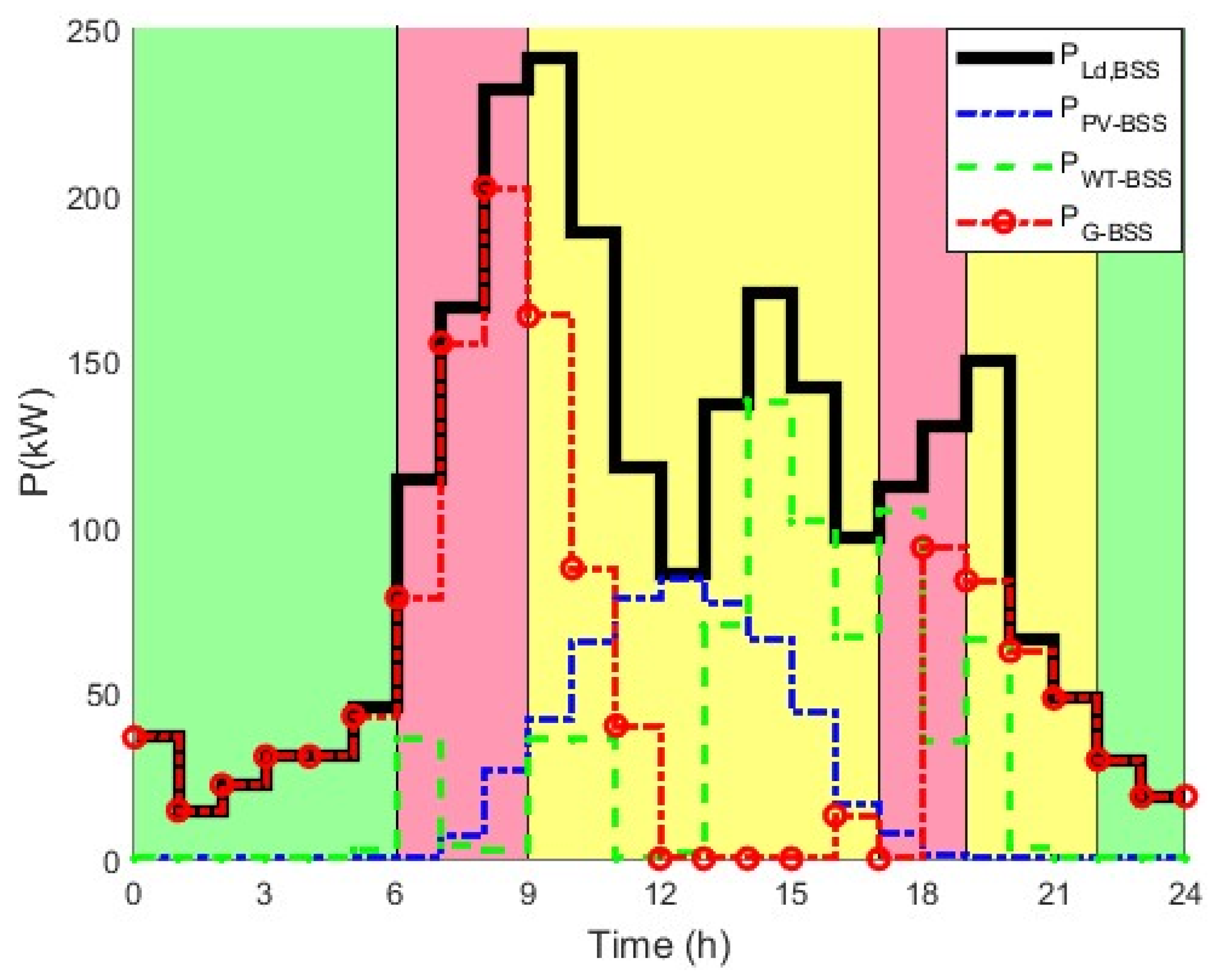
3.1. EV BSS Power Demand Load Profile

To accurately assess the energy requirements of the EV BSS, a detailed load profile was constructed using historical data from an operational BSS. The chosen EV BSS is a heavy-duty truck swapping station situated at a central logistics hub in Shanghai Port, China, where energy consumption patterns reflect the high and variable demand associated with commercial EV operations. The data were recorded over a representative period, capturing daily and seasonal demand variations. Figure 3 illustrates the daily energy consumption at the EV BSS, highlighting peak demand periods that coincide with high traffic volumes and operational hours. The background colors in Figure 3 are designated as green for off-peak, yellow for standard, and light red for peak periods. The load profile serves as the basis for sizing the hybrid renewable energy system and determining the optimal mix of energy sources.

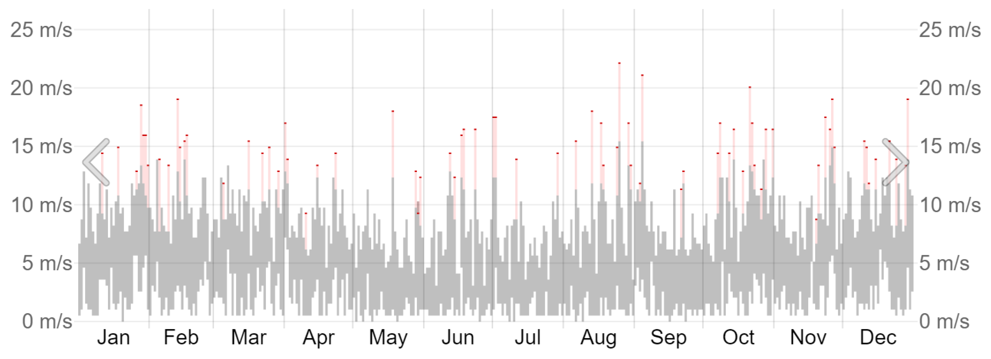
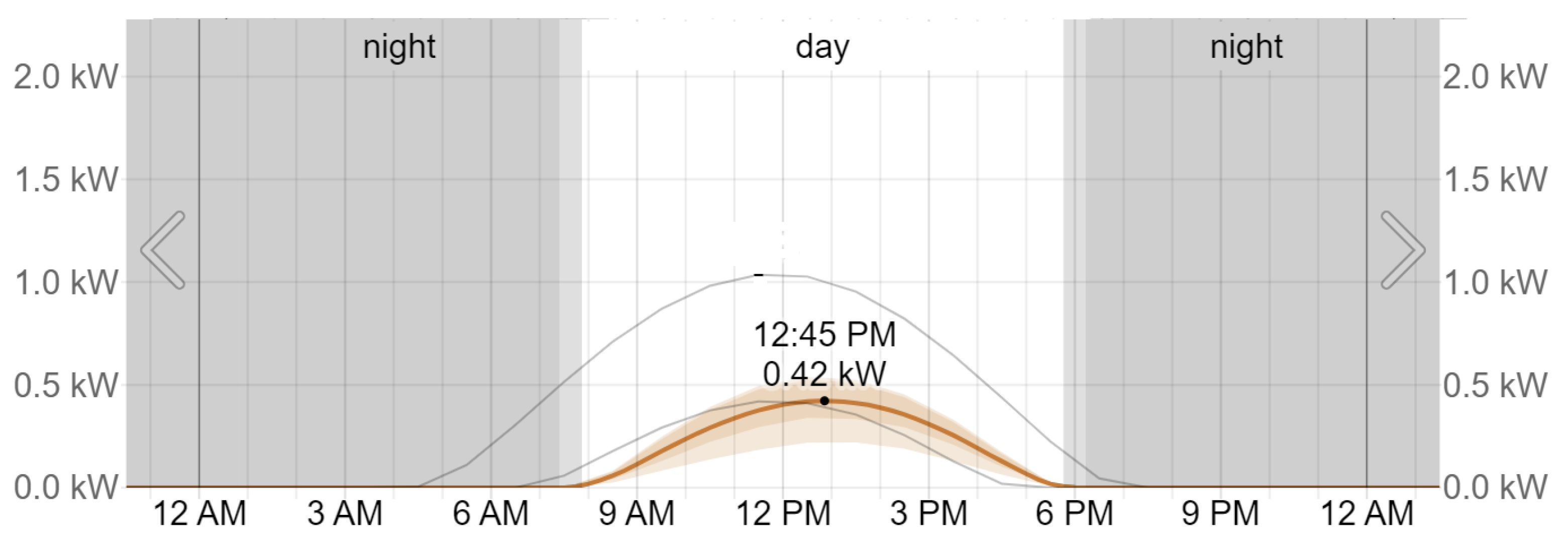
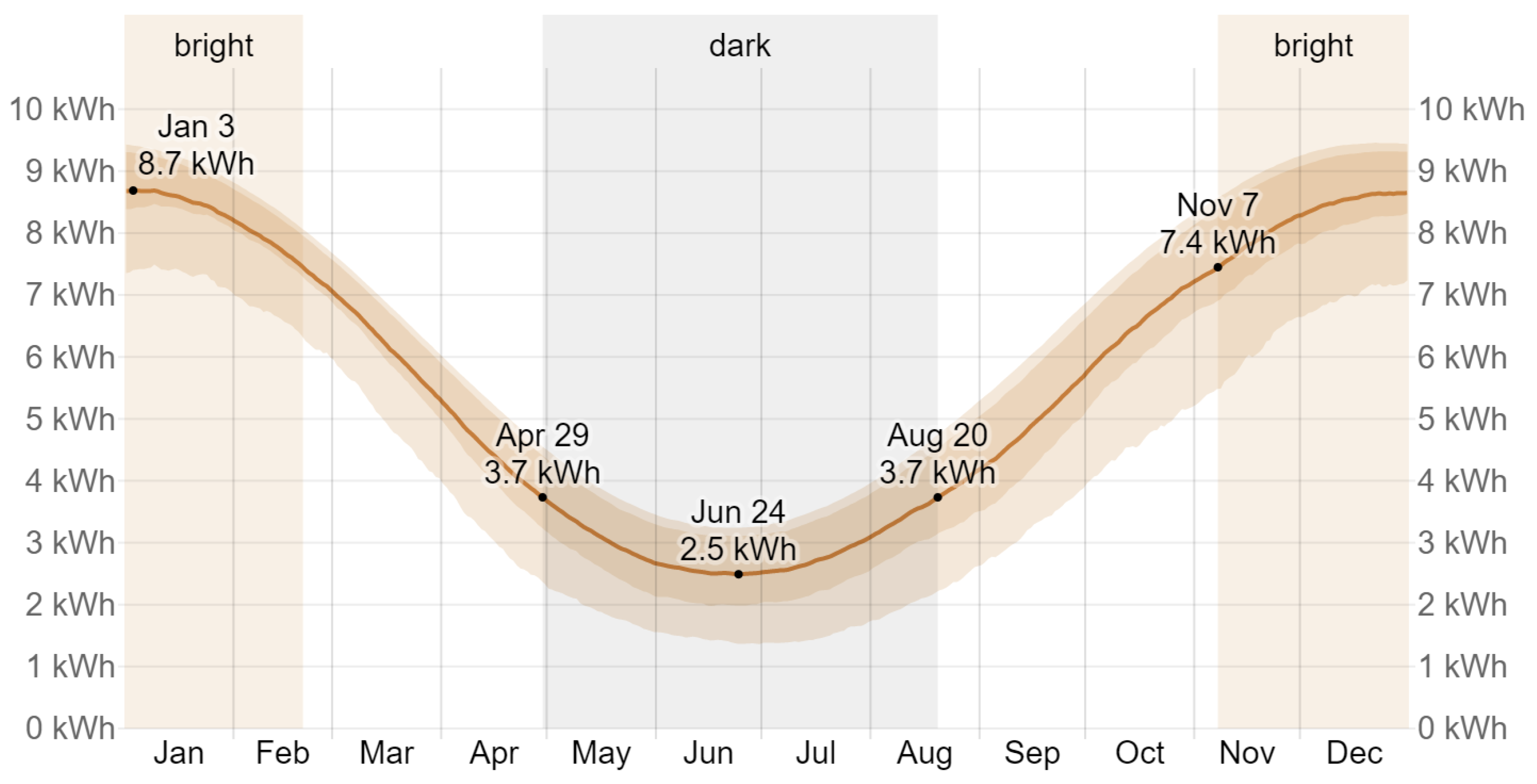
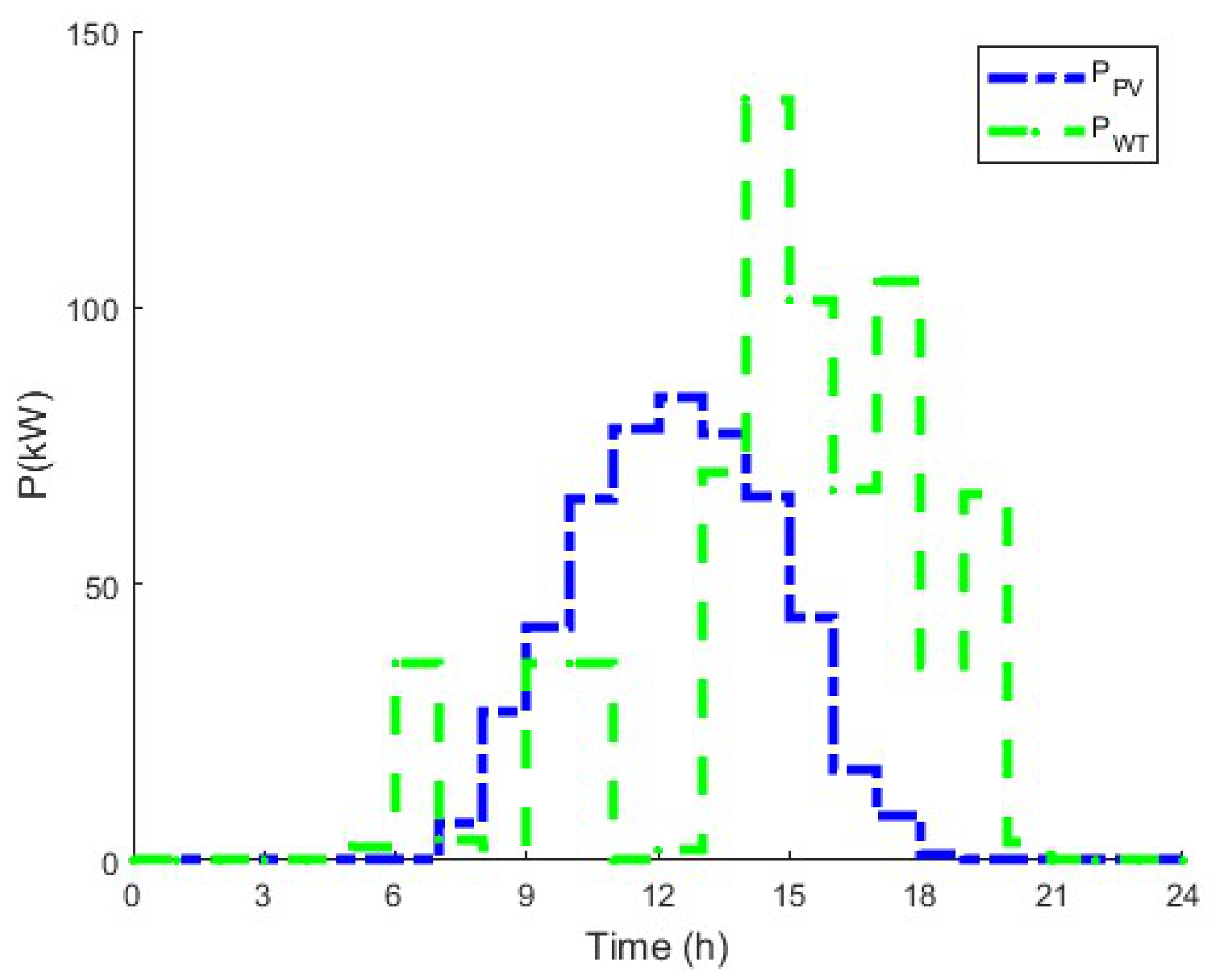
3.2. Renewable Energy Power Supply

The proposed hybrid system incorporates WTs and solar PV panels as primary energy sources, supplemented by grid electricity, to ensure a reliable supply. The input parameters for WT system power generation, such as the wind speed, and for solar PV power generation, such as the solar radiation and ambient temperature, are obtained from a typical day in the low-demand season in Cape Town, South Africa, as referenced in [69]. Figure 4 illustrates the hourly average wind speed measured at a height of 10 m above ground level. The wind speed varies throughout the day, with a daily average of 2.46 m/s. The windiest period occurs between 2:00 and 3:00 PM, with an average wind speed of 4.6 m/s, while the calmest period is observed between 1:00 and 2:00 AM, with an average wind speed of 1.08 m/s. For more information, the average hourly wind speed over the year is presented in Figure 5. Additionally, the daily average for PV generation is depicted in Figure 6, indicating that the peak incident shortwave radiation for solar PV power generation reaching the ground’s surface over a wide area is approximately 0.42 ${\mathrm{kW}/\mathrm{m}}^2$ around 12:45 PM. For more information, the annual shortwave radiation for solar PV power generation reaching the ground’s surface over a wide area is presented in Figure 7, which provides significant seasonal variation, with the brightest peak around December and the darkest period around June. respectively. The proposed hybrid power system is designed to ensure that the EV BSS charging demand is met at any given time, particularly when electricity from the utility grid is expensive. The sizing of the WT and solar PV system is tied to the initial equipment cost and available capital, directly impacting power generation and reducing energy costs from the utility grid.

3.3. Time-of-Use Electricity Tariff

The South African power grid is operated by the national utility company “Eskom”, Sandton, South Africa, while electricity tariffs are regulated by the National Energy Regulator of South Africa (NERSA). Eskom’s tariff structure typically includes both flat and dynamic TOU pricing systems. TOU pricing is a demand-side management strategy that reflects the varying costs of electricity production throughout the day and is divided into three periods: off-peak ($p_{e off}$), standard-peak ($p_{e std}$), and on-peak ($p_{e pk}$). These periods correspond to times when electricity demand and generation costs are low, moderate, and high, respectively. In the context of the optimization problem, the TOU electricity tariff significantly influences the energy efficiency of the EV BSS. This paper considers the Eskom Megaflex TOU tariff scheme, which applies to urban and industrial consumers who both consume energy from the utility grid and generate energy at the same point of supply. For this case study, the 2023/2024 Eskom Megaflex electricity tariff for high-demand season (from June to August) weekdays is used as the basis for the TOU electricity tariff analysis provided in [70].

$$p_{e\left(t\right)}=\left\{\begin{array}{c}{p}_{e off}=1.0370 ZAR/\mathrm{kWh} ; \mathrm{if} \mathrm{t}\in [00:00,06:00)\cup [22:00,24:00),\hfill \\ p_{e std}=1.8991 ZAR/\mathrm{kWh} ; \mathrm{if} \mathrm{t}\in [09:00,17:00)\cup [19:00,22:00),\hfill \\ p_{e pk}=6.2421 ZAR/\mathrm{kWh} ; \mathrm{if} \mathrm{t}\in [06:00,09:00)\cup [17:00,19:00).\hfill \end{array}\right.$$

(57)

with $ZAR$ being the South African currency (Rand) and t representing the time of day in hours.

4. Simulation Results and Discussion

The following section breaks down the simulation results from the optimization model presented in the previous section. The simulation results regarding the system’s performance, cost-effectiveness, and reliability are analyzed. Additionally, the impact of varying key input parameters, such as the number of WTs, PV panels, and TOU electricity tariffs, is also discussed. The outcomes provide insights into the optimal design and management strategies for a grid-connected wind–solar hybrid power supply system for the EV BSS. Furthermore, a comprehensive economic analysis is conducted by assessing the payback period and cost-effectiveness of installing the proposed system.

4.1. Optimal Hybrid Power System Sizing and Management Strategy

The optimization problem, formulated as an MILP, is solved through the SCIP solver within MATLAB’s R2024a OPTI Toolbox during a 24 h horizon with a sampling interval $\Delta t$ = 1 h. The objective is to determine the most cost-effective and reliable design for the hybrid system, focusing on the optimal sizing of WTs and solar PV panels to meet the charging demand while minimizing reliance on the utility grid. The simulation utilized technical and economic input parameters, as outlined in

Table 1. Simulation parameters used in this paper.

Parameters	Symbol	Values
Installation lifetime	$L_p$	20 years
Sampling period	N	24
Sampling time	$\Delta t$	1 h
Weighting factor	$\xi$	0.5
Upper bound	$ub$	$[481 2802 \infty ]$
Lower bound	$lb$	$[0 0 0 ]$
Inflation rate	r	4.60%
Interest rate	i	8.25%
Photovoltaic systems
Lifetime of the PV system	$L_{PV}$	25 years
Rated power of the PV panel	$P{r}_{PV}$	0.545 kW
Conversion efficiency of the PV panel	${\eta }_{PV}$	19.4%
Rated efficiency of the PV panel	${\eta }_r$	18.1%
Initial cost of the PV panel	$I{C}_{INVT,PV}$	ZAR 3199.99
Annual O & M cost of PV	$C_{O\&M{,}_{PV}}$	1% of $I{C}_{INVT,PV}$
Capital cost of the solar PV per kW	$\delta$	ZAR 8220.16/kW
Wind turbine systems
Lifetime of the WT system	$L_{WT}$	25 years
Rated power of the WT generator	$P{r}_{WT}$	8 kW
Rated WT speed	$V_r$	12 m/s
Cut-in WT speed	$V_{ci}$	2.5 m/s
Cut-out WT speed	$V_{co}$	25 m/s
WT gearbox efficiency	${\eta }_T$	90%
WT generator efficiency	${\eta }_g$	80%
Air density	${\phi }_a$	1.225 kg/m3
WT power coefficient	$C_p$	0.48
Initial cost of the WT	$I{C}_{INVT,WT}$	ZAR 10,580.63
Annual O & M cost of WT	$C_{O\&M{,}_{WT}}$	5% of $I{C}_{INVT,WT}$
Capital cost of the WT per kW	$\gamma$	ZAR 15,403/kW
Inverter
Lifetime of the inverter	$L_{INV}$	15 Years
Efficiency of the inverter	${\eta }_{INV}$	98%
Inverter factor	$K_{INV}$	1.25
Initial cost of the inverter	$I_{C,INV}$	ZAR 38,860.00
Capital cost of inverter per kW	$\lambda$	ZAR 3 108.80/kW

, to identify the optimal configuration of the hybrid system. With a weighting factor of 0.5, the simulation results indicate that the optimal configuration for the hybrid systems consists of 64 WTs and 402 solar PV panels, resulting in a total LCC of ZAR 1,963,520.12. This configuration remains optimal for weighting factor values within the range of 0.27 to 0.71. For weighting factors below 0.27, the hybrid system is prioritized over the utility grid, potentially leading to excess energy absorbed by the utility grid. Conversely, weighting factors above 0.71 prioritize the utility grid, resulting in an oversized hybrid system with all the charging power supplied by the utility grid.

Figure 8 illustrates the power generated by the hybrid power system over a 24 h period. It shows that both wind and PV power sources exhibit diurnal patterns, with peaks occurring at different times of the day. The PV power generation starts increasing in the morning, reaching its peak between 12:00 and 15:00 when solar irradiance is at its highest. It gradually decreases towards the evening as sunlight diminishes, showing a typical bell-shaped curve. In contrast, the WT power output exhibits more variability throughout the day, with multiple peaks occurring at different times, reflecting the intermittent nature of wind speed. Notably, wind power generation complements the PV output by producing power during the early morning and late afternoon hours when solar power is negligible, demonstrating a synergistic effect that enhances the overall renewable energy availability. This complementary behavior benefits hybrid renewable systems as it can reduce dependency on grid power.

Figure 9 presents the simulation results of the charging demand along with the optimal output power flows from each source over a 24 h period. It can be observed that the charging demand fluctuates throughout the 24 h, with peak demands occurring around 10 AM, 3 PM, and 8 PM. Hybrid power generation systems supply a significant portion of the power required to meet this charging demand, thereby substantially reducing the operational costs associated with the utility grid. During the off-peak hours (00:00–06:00), hybrid power generation is minimal due to low wind speeds and the unavailability of solar PV, resulting in higher reliance on the utility grid to meet the charging demand. As the wind speed increases from 06:00 onwards, WTs contribute more significantly to the power supply, reducing utility grid dependency. The solar PV system begins generating power at sunrise, reaching its peak around noon. During these hours, the combined contribution of solar PV and WTs is sufficient to meet the charging demand of the EV BSS, significantly decreasing the operational cost of the system. The utility grid supplements any remaining deficit power. Between 17:00 and 19:00, there is another peak in charging demand. Solar PV generation declines at this time, and WTs partially compensate for the power deficit. However, some reliance on the utility grid is necessary to meet the demand. The system’s optimization strategy ensures that electricity is predominantly drawn from renewable sources whenever available, limiting the use of expensive grid electricity during peak TOU tariff periods.

Applying Eskom’s TOU electricity tariff to the proposed system generates a daily electricity cost of R7 676.39 for the charging demand. Incorporating the optimization model reduces this cost to ZAR 4483.53, representing 41.6% of the daily cost savings.

Table 2. Simulation results of the proposed system.

Number of WTs	Number of PV Panels	Total Life Cycle Cost
64	402	ZAR 1,963,520.12

and

Table 3. Daily and annual cost savings of the proposed system.

	Baseline	Optimal	Saving
Daily cost	ZAR 7676.39	ZAR 4483.53	ZAR 3192.5
Annualized cost			ZAR 1,165,262.5

summarize the simulation results, including the number of WTs, PV panels, total LCC, and cost savings achieved through optimal control intervention. These results are based on the average daily cost in the case study, with the daily cost annualized to reflect an average yearly amount. The results demonstrate the feasibility and effectiveness of integrating wind and solar energy, significantly reducing the dependency on the utility grid and offering a sustainable and resilient solution for EV charging and swapping infrastructure.

The proposed optimization model is tailored to a specific region but has been demonstrated as operational in the existing literature. An analysis of the methodology and simulation results indicates that the model effectively demonstrates the techno-economic feasibility and provides an optimal design approach for managing grid-connected hybrid power generation systems in EV BSSs over multiple days under different operational scenarios. Although the optimization model is designed for a particular use case, the simulation results suggest that its straightforward structure enables adaptation to a more generalized framework that is applicable to various electricity markets.

The study’s findings highlight that integrating grid-connected hybrid wind–PV systems into EV BSSs aligns with South Africa’s energy objectives, particularly the Integrated Resource Plan (IRP, 2019) [71], which emphasizes RE diversification and emission reductions in the transport sector. These findings augment the country’s broader policy aspirations of reducing dependence on fossil fuels and implementing distributed generation systems, promoting energy security through minimized grid dependency. To fully capture such innovations, strategic policy changes are required. Governments can provide economic incentives, such as tax rebates and low-interest loans, to help lower hybrid system adoption barriers. Streamlining the permitting procedure and reforming TOU tariff prices would also promote off-peak RE consumption, matching economic benefits with sustainable strategies. Encouraging public–private partnerships and investing in adaptive grid technologies could create a regulatory environment that accelerates infrastructure development with rapid technological advancements. Collaboration among policymakers, utilities (e.g., Eskom), and private stakeholders is equally vital. Collaborative efforts in co-funding pilot trials and developing harmonized technical standards would close the gap between research and large-scale deployment and align with national climate change policies [71] and energy security agendas.

4.2. LCC Analysis for the Payback Period

Economic feasibility is assessed through a cost–benefit analysis of cash outflows and inflows associated with installing the proposed system. The installation feasibility can be evaluated using various methods, considering both environmental benefits and economic indicators [72,73,74]. The LCC method considers the time value of money and the lifespan of the installation by converting all the future cash flows into their present value through discounting. The comparative advantage of LCC is that it covers all the cash inflows and outflows into the system in its lifetime. As a result, the discounted present value (DPV) of a cash flow occurring in a future period (z-th year) can be expressed as

$$DPV\left(z\right)={\displaystyle \frac{FV\left(z\right)}{{(1+d)}^z}}$$

(58)

where $DPV$ is the discounted present value of the future cash flow, $FV$ is the nominal value of a cash flow amount in a future period (z-th year), d is the discount rate, and z is the time in years before the future cash flow occurs. In this LCC analysis, d represents the time value of money or the cost of holding capital and may also account for the risk of not receiving the full payment. The actual d is calculated as the difference between the average interest rate and the inflation rate. The interest rate (r) reflects the opportunity cost of time, representing the compensation required to delay spending from the current to a future year. On the other hand, the inflation rate (i) indicates the percentage change in prices over a specific period, typically measured monthly or annually, and shows how quickly prices increased during that time. The i is an essential parameter in the LCC analysis of an installation project, and, thus, the unit cost of generation is an essential parameter. In this paper, the average interest rate [75] is 8.25%, and the inflation rate [76] is 4.6%, reflecting the time value of money in South Africa as of July 2024. The component prices are based on South African market rates. In this LCC economic analysis of energy efficiency projects, both operational and maintenance costs, as well as cost savings, are considered. Once FV (z) is determined, the net present value (cumulative cash flow) is calculated as follows [74]:

$$NP{V}_{z=1}^m=\sum _{z=1}^{m}DPV\left(z\right)-CC$$

(59)

where NPV is the net present value (or cumulative cash flow) and CC is the total investment capital cost. Subsequently, the discounted payback period (PBP) can be determined using the following equation [74]:

$$PBP=m_y+{\displaystyle \frac{-NP{V}_{z=1}^m}{DPV(m_y+1)}}$$

(60)

where $m_y$ denotes the last year with a negative NPV.

Table 4. Cost components of the proposed system.

Components	Costs (ZAR)
Wind turbines	677,160.32
Solar photovoltaic	1,286,359.80
Inverters	77,720
Installation cost	649,975.98
Accessories	3,000,000
Total investment capital cost	5,691,216.10

provides the approximate prices of the various components of the proposed system, leading to a total investment capital cost.

Certain assumptions are made when conducting the LCC analysis for the proposed system. It is assumed that the annual operation and maintenance costs $C_{O\&M}$, as well as the annual optimal cost–benefit, will increase proportionally over the installation service lifetime. The annual cost–benefit represents the amount the EV BSS owner would have spent each year without implementing the proposed system.

Table 5. Life cycle cost analysis and payback period of the proposed system with a total investment capital cost of ZAR 5,691,216.10.

Years	Annual O & M Cost (ZAR)	Annual Optimal Cost–Benefit (ZAR)	Total	Discount Factor ${(1+\mathrm{d})}^{-{\mathit{L}}_{\mathit{p}}}$	Discounted Cash Flows	Cumulative Cash Flows
0				1.00	(5,691,216.10)	(5,691,216.10)
1	(46,721.61)	1,165,390.25	1,118,668.64	0.96	1,079,275.10	(4,611,941.01)
2	(47,389.73)	1,182,055.33	1,134,665.60	0.93	1,056,158.93	(3,555,782.07)
3	(48,067.40)	1,198,958.72	1,150,891.32	0.90	1,033,537.87	(2,522,244.20)
4	(48,754.77)	1,216,103.83	1,167,349.07	0.87	1,011,401.32	(1,510,842.89)
5	(49,451.96)	1,233,494.12	1,184,042.16	0.84	989,738.89	(521,104.00)
6	(50,159.12)	1,251,133.08	1,200,973.96	0.81	968 540.43	447,436.43
7	(50,876.40)	1,269,024.29	1,218,147.89	0.78	947,796.00	1,395,232.43
8	(51,603.93)	1,287,171.33	1,235,567.40	0.75	927 495.88	2,322,728.31
9	(52,341.87)	1,305,577.88	1,253,236.02	0.72	907 630.56	3,230,358.87
10	(53,090.35)	1,324,247.65	1,271,157.29	0.70	788,190.71	4,018,549.58
11	(53,849.55)	1,343,184.39	1,289,334.84	0.67	869,167.24	4,887,716.82
12	(54,619.60)	1,362,391.92	1,307,772.33	0.65	850,551.21	5,738,268.03
13	(55,400.66)	1,381,874.13	1,326,473.47	0.63	832,333.90	6,570,601.93
14	(56,192.89)	1,401,634.93	1,345,442.04	0.61	814 506.78	7,385,108.72
15	(56,996.44)	1,421,678.31	1,364,681.86	0.58	797,061.48	8,182,170.20
16	(57,811.49)	1,442 008.31	1,384,196.82	0.56	779,989.84	8,962,160.04
17	(58,638.20)	1,462,629.03	1,403,990.83	0.54	763,283.83	9,725,443.87
18	(59,476.72)	1,483,544.62	1,424,067.90	0.52	746,935.64	10,472,379.50
19	(60,327.24)	1,504,759.31	1,444,432.07	0.51	730,937.60	11,203,317.10
20	(61,189.92)	1,526,277.37	1,465,087.45	0.49	715,282.20	11,918,599.30
Payback is 5 years plus 6 months (6.45636)

presents the LCC analysis of the proposed system under the optimal control strategy, with the salvage cost neglected when calculating the PBP. As shown in Table 5, the projected total investment capital cost is recorded as a negative cash flow in brackets as (ZAR 5,691,216.10) in the financial statement. The cash flows and PBP are calculated following the assumptions that the annual optimal cost–benefit and $C_{O\&M}$ will increase proportionately during the lifetime of the proposed system. The cumulative cash flows decrease as negative ones until they eventually turn positive. The payback occurs when the cumulative cash flow reaches zero, and, at this point, the total invested capital cost has been fully recovered. For the proposed system, the PBP occurs after 5 years and 6 months. Afterward, the cumulative cash flow becomes positive, and all the revenue in the following years represents pure profit or benefit. Suppose that the proposed system installation has a lifetime of 20 years and a payback period of approximately 5 years and 6 months. In that case, the EV BSS owner can recover the total capital investment within a reasonable timeframe and will have over 10 years to generate guaranteed profit.

5. Conclusions

This paper presents a novel techno-economic evaluation and optimal design approach for a grid-connected wind–photovoltaic hybrid power generation system tailored for electric vehicle battery swapping stations. The proposed optimization model, developed using mixed-integer linear programming, aims to minimize the total life cycle cost and the cost of electrical energy consumption from the utility grid while maximizing system reliability. By considering decision variables such as the number of wind turbines, solar photovoltaic panels, and power drawn from the utility grid, the model provides a comprehensive solution for cost-effective energy management. For the case study, the simulation results reveal the optimal configuration of 64 wind turbines and 402 solar photovoltaic panels, leading to a total life cycle cost of ZAR 1,963,520.12, achieving substantial energy cost savings of 41.58% through effective energy cost management under a time-of-use electricity tariff. Additionally, the life cycle cost analysis, as the economic performance indicator, reveals a payback period of 5 years and 6 months, affirming the economic viability of the proposed hybrid system. This optimization approach substantially reduces energy costs and enhances system reliability. Such techno-economic feasibility and design optimization provide an adaptable solution for various applications. The developed method can be extended to different locations, proving its flexibility in optimizing grid-connected wind–photovoltaic hybrid power systems, especially in areas where the energy storage costs may be prohibitive. The proposed system offers a reliable and cost-effective solution for electric vehicle battery swapping stations, with promising potential for widespread implementation on South African highways, delivering both economic and environmental benefits.

References

1. Skovgaard, J. EU climate policy after the crisis. Environ. Politics 2014, 23, 1–17. [Google Scholar] [CrossRef]
2. McCarthy, J. A socioecological fix to capitalist crisis and climate change? The possibilities and limits of renewable energy. Environ. Plan. Econ. Space 2015, 47, 2485–2502. [Google Scholar] [CrossRef]
3. Eder, L.; Provornaya, I. Analysis of energy intensity trend as a tool for long-term forecasting of energy consumption. Energy Effciency 2018, 11, 1971–1997. [Google Scholar] [CrossRef]
4. Kenny, A. The rise and fall of Eskom and how to fix it now. Policy Bull. S. Afr. Inst. Race Relat. 2015, 2, 1–22. [Google Scholar]
5. Giglmayr, S.; Brent, A.C.; Gauché, P.; Fechner, H. Utility-scale PV power and energy supply outlook for South Africa in 2015. Renew. Energy 2015, 83, 779–785. [Google Scholar] [CrossRef]
6. Alexander, M.; Tonachel, L. Projected greenhouse gas emissions for plug-in electric vehicles. World Electr. Veh. J. 2016, 8, 987–995. [Google Scholar] [CrossRef]
7. Sujitha, N.; Krithiga, S. Res based ev battery charging system: A review. Renew. Sustain. Energy Rev. 2017, 75, 978–988. [Google Scholar] [CrossRef]
8. International Energy Agency. Global EV Outlook 2021. Available online: https://www.iea.org/reports/global-ev-outlook-2021 (accessed on 25 April 2023).
9. Vani, B.V.; Kishan, D.; Ahmad, M.W.; Reddy, C.R.P. Enhanced electric vehicle battery management system employing bat algorithm with chaotic diversification strategies. IET Power Electron. 2024, 17, 2319–2330. [Google Scholar] [CrossRef]
10. Sui, Q.; Li, F.; Wu, C.; Feng, Z.; Lin, X.; Wei, F.; Li, Z. Optimal scheduling of battery charging–swapping systems for distribution network resilience enhancement. Energy Rep. 2022, 8, 6161–6170. [Google Scholar] [CrossRef]
11. Revankar, S.R.; Kalkhambkar, V.N. Grid integration of battery swapping station: A review. J. Energy Storage 2021, 41, 102937. [Google Scholar] [CrossRef]
12. Macharia, V.M.; Garg, V.K.; Kumar, D. A review of electric vehicle technology: Architectures, battery technology and its management system, relevant standards, application of artificial intelligence, cyber security, and interoperability challenges. IET Electr. Syst. Transp. 2023, 13, 12083. [Google Scholar] [CrossRef]
13. Nyamayoka, L.T.; Masisi, L.M.; Dorrell, D.G.; Wang, S. Optimisation Design of On-Grid Hybrid Power Supply System for Electric Vehicle Battery Swapping Station. In Proceedings of the 2023 IEEE International Future Energy Electronics Conference (IFEEC), Sydney, Australia, 20–23 November 2023; pp. 296–299. [Google Scholar]
14. Alanazi, F. Electric Vehicles: Benefits, Challenges, and Potential Solutions for Widespread Adaptation. Appl. Sci. 2023, 13, 6016. [Google Scholar] [CrossRef]
15. Zhan, W.; Wang, Z.; Zhang, L.; Liu, P.; Cui, D.; Dorrell, D.G. A review of siting, sizing, optimal scheduling, and cost-benefit analysis for battery swapping stations. Energy 2022, 258, 124723. [Google Scholar] [CrossRef]
16. Horak, D.; Hainoun, A.; Neugebauer, G.; Stoeglehner, G. Battery electric vehicle energy demand in urban energy system modeling: A stochastic analysis of added flexibility for home charging and battery swapping stations. Sustain. Energy Grids Netw. 2024, 37, 01260. [Google Scholar] [CrossRef]
17. Li, Y.; Zhu, F.; Li, L.; Ouyang, M. Electrifying heavy-duty truck through battery swapping. Joule 2024, 8, 1556–1561. [Google Scholar] [CrossRef]
18. Sehar, F.; Pipattanasomporn, M.; Rahman, S. Demand management to mitigate impacts of plug-in electric vehicle fast charge in buildings with renewables. Energy 2017, 120, 642–651. [Google Scholar] [CrossRef]
19. Amiri, S.S.; Jadid, S.; Saboori, H. Multi-objective optimum charging management of electric vehicles through battery swapping stations. Energy 2018, 15, 549–562. [Google Scholar] [CrossRef]
20. Adu-Gyamfi, G.; Song, H.; Nketiah, E.; Obuobi, B.; Adjei, M.; Cudjoe, D. Determinants of adoption intention of battery swap technology for electric vehicles. Energy 2022, 15, 123862. [Google Scholar] [CrossRef]
21. Danilovic, M.; Liu, J.L.; Müllern, T.; Nåbo, A.; Almestrand Linné, P. Exploring Battery-Swapping for Electric Vehicles in China 1.0. Sweden-China Bridge. March 2021, pp. 1–105. Available online: https://www.diva-portal.org/smash/get/diva2:1628149/FULLTEXT01.pdf (accessed on 6 November 2023).
22. Chen, X.; Xing, K.; Ni, F.; Wu, Y.; Xia, Y. An electric vehicle battery-swapping system: Concept, architectures, and implementations. IEEE Intell. Transp. Syst. Mag. 2021, 14, 175–194. [Google Scholar] [CrossRef]
23. Lebrouhi, B.E.; Khattari, Y.; Lamrani, B.; Maaroufi, M.; Zeraouli, Y.; Kousksou, T. Key challenges for a large-scale development of battery electric vehicles: A comprehensive review. J. Energy Storage 2021, 44, 103273. [Google Scholar] [CrossRef]
24. Shalaby, A.A.; Shaaban, M.F.; Mokhtar, M.; Zeineldin, H.H.; El-Saadany, E.F. A dynamic optimal battery swapping mechanism for electric vehicles using an LSTM-based rolling horizon approach. IEEE Trans. Intell. Transp. Syst. 2022, 23, 15218–15232. [Google Scholar] [CrossRef]
25. Boonraksa, T.; Boonraksa, P.; Pinthurat, W.; Marungsri, B. Optimal Battery charging schedule for a battery swapping station of an electric bus with a PV integration considering energy costs and peak-to-average ratio. IEEE Access 2024, 12, 36280–36295. [Google Scholar] [CrossRef]
26. Yan, J.; Menghwar, M.; Asghar, E.; Panjwani, M.K.; Liu, Y. Real-time energy management for a smart-community microgrid with battery swapping and renewables. Appl. Energy 2019, 238, 180–194. [Google Scholar] [CrossRef]
27. Mahoor, M.; Hosseini, Z.S.; Khodaei, A. Least-cost operation of a battery swapping station with random customer requests. Energy 2019, 172, 913–921. [Google Scholar] [CrossRef]
28. Liu, X.; Zhao, T.; Yao, S.; Soh, C.B.; Wang, P. Distributed operation management of battery swapping-charging systems. IEEE Trans. Smart Grid 2018, 10, 5320–5333. [Google Scholar] [CrossRef]
29. Bian, H.; Ren, Q.; Guo, Z.; Zhou, C. Optimal Scheduling of Integrated Energy System Considering Electric Vehicle Battery Swapping Station and Multiple Uncertainties. World Electr. Veh. J. 2024, 15, 170. [Google Scholar] [CrossRef]
30. Jordehi, A.R.; Javadi, M.S.; Catalão, J.P. Optimal placement of battery swap stations in microgrids with micro pumped hydro storage systems, photovoltaic, wind and geothermal distributed generators. Int. J. Electr. Power Energy Syst. 2021, 125, 106483. [Google Scholar] [CrossRef]
31. Ren, L.; Liao, W.; Chen, J. Systematic Design and Implementation Method of Battery-Energy Comprehensive Management Platform in Charging and Swapping Scenarios. Energies 2024, 17, 1237. [Google Scholar] [CrossRef]
32. Wu, S.; Xu, Q.; Li, Q.; Yuan, X.; Chen, B. An optimal charging strategy for pv based battery swapping stations in a dc distribution system. Int. J. Photoenergy 2017, 2017, 1504857. [Google Scholar] [CrossRef]
33. Gull, M.S.; Khalid, M.; Arshad, N. Multi-objective optimization of battery swapping station to power up mobile and stationary loads. Appl. Energy 2024, 374, 124064. [Google Scholar] [CrossRef]
34. Fachrizal, R.; Shepero, M.; Åberg, M.; Munkhammar, J. Optimal PV-EV sizing at solar powered workplace charging stations with smart charging schemes considering self-consumption and self-sufficiency balance. Appl. Energy 2022, 307, 118139. [Google Scholar] [CrossRef]
35. DoT. Green Transport Strategy for South Africa: (2018–2050); Department of Transport: Pretoria, South Africa, 2019.
36. Ahjum, F.; Godinho, C.; Burton, J.; McCall, B.; Marquard, A. A Low-Carbon Transport Future for South Africa: Technical, Economic and Policy Considerations; Climate Transparency: Cape Town, South Africa, 2020; pp. 1–28. [Google Scholar]
37. Pillay, N.S.; Nassiep, S. Employment in Automotive Parts with Electric Vehicle Market Penetration in South Africa. 2020. Available online: https://proceedings.systemdynamics.org/2020/papers/P1016.pdf (accessed on 15 September 2023).
38. Moeletsi, M.E.; Tongwane, M.I. Projected direct carbon dioxide emission reductions as a result of the adoption of electric vehicles in Gauteng province of South Africa. Atmosphere 2020, 11, 591. [Google Scholar] [CrossRef]
39. Lamedica, R.; Santini, E.; Ruvio, A.; Palagi, L.; Rossetta, I. A MILP methodology to optimize sizing of PV-Wind renewable energy systems. Energy 2018, 165, 385–398. [Google Scholar] [CrossRef]
40. Banks, D.; Schaffler, J. The Potential Contribution of Renewable Energy in South Africa. In Sustainable Energy & Climate Change Project (SECCP); 2005; pp. 1–116. Available online: https://earthlife-ct.org.za/downloads/The_Potential_Contribution_of_Renewable_Energy_in_South_Africa.pdf (accessed on 19 January 2025).
41. Diaf, S.; Belhamel, M.; Haddadi, M.; Louche, A. Technical and economic assessment of hybrid photovoltaic/wind system with battery storage in corsica island. Energy Policy 2008, 36, 743–754. [Google Scholar] [CrossRef]
42. Diaf, S.; Diaf, D.; Belhamel, M.; Haddadi, M.; Louche, A. A methodology for optimal sizing of autonomous hybrid pv/wind system. Energy Policy 2007, 35, 5708–5718. [Google Scholar] [CrossRef]
43. Belkaid, A.; Colak, I.; Isik, O. Photovoltaic maximum power point tracking under fast varying of solar radiation. Appl. Energy 2016, 179, 523–530. [Google Scholar] [CrossRef]
44. Abbes, D.; Martinez, A.; Champenois, G. Life cycle cost, embodied energy and loss of power supply probability for the optimal design of hybrid power systems. Math. Comput. Simul. 2014, 98, 46–62. [Google Scholar] [CrossRef]
45. Kazem, H.A.; Khatib, T. Techno-economical assessment of grid connected photovoltaic power systems productivity in Sohar, Oman. Sustain. Energy Technol. Assess. 2013, 3, 6–65. [Google Scholar] [CrossRef]
46. Ramli, M.A.; Hiendro, A.; Twaha, S. Economic analysis of pv/diesel hybrid system with flywheel energy storage. Renew. Energy 2015, 78, 398–405. [Google Scholar] [CrossRef]
47. Bokopane, L.; Kanzumba, K.; Vermaak, H. Is the south african electrical infrastructure ready for electric vehicles? In 2019 Open Innovations (OI); IEEE: Cape Town, South Africa, 2019; pp. 127–131. [Google Scholar]
48. Dane, A.; Wright, D.; Montmasson-Clair, G. Exploring the Policy Impacts of a Transition to Electric Vehicles in South Africa; Trade & Industrial Policy Strategies: Pretoria, South Africa, 2019; pp. 1–20. [Google Scholar]
49. Sooknanan, P.N.; Brent, A.C.; Musango, J.K.; van Geems, F. Using a system dynamics modelling process to determine the impact of ecar, ebus and etruck market penetration on carbon emissions in South Africa. Energies 2020, 13, 575. [Google Scholar] [CrossRef]
50. Brenna, M.; Foiadelli, F.; Leone, C.; Longo, M. Electric vehicles charging technology review and optimal size estimation. J. Electr. Eng. Technol. 2020, 15, 2539–2552. [Google Scholar] [CrossRef]
51. Hemmati, R. Chapter 3—Integration of electric vehicles and charging stations. In Energy Management in Homes and Residential Microgrids: Short-Term Scheduling and Long-Term Planning; Hemmati, R., Ed.; Elsevier: Amsterdam, The Netherlands, 2024; pp. 79–140. [Google Scholar]
52. Evans, A.; Strezov, V.; Evans, T.J. Assessment of sustainability indicators for renewable energy technologies. Renew. Sustain. Energy Rev. 2009, 13, 1082–1088. [Google Scholar] [CrossRef]
53. Adefarati, T.; Bansal, R.C.; Shongwe, T.; Naidoo, R.; Bettayeb, M.; Onaolapo, A.K. Optimal energy management, technical, economic, social, political and environmental benefit analysis of a grid-connected PV/WT/FC hybrid energy system. Energy Convers. Manag. 2023, 292, 117390. [Google Scholar] [CrossRef]
54. Al-Sharrah, G.; Elkamel, A.; Almanssoor, A. Sustainability indicators for decision-making and optimisation in the process industry: The case of the petrochemical industry. Chem. Eng. Sci. 2010, 65, 1452–1461. [Google Scholar] [CrossRef]
55. Bilal, M.; Oladigbolu, J.O.; Mujeeb, A.; Al-Turki, Y.A. Cost-effective optimization of on-grid electric vehicle charging systems with integrated renewable energy and energy storage: An economic and reliability analysis. J. Energy Storage 2024, 100, 113170. [Google Scholar] [CrossRef]
56. Sediqi, M.M.; Furukakoi, M.; Lotfy, M.E.; Yona, A.; Senjyu, T. Optimal economical sizing of grid-connected hybrid renewable energy system. J. Energy Power Eng. 2017, 11, 244–253. [Google Scholar]
57. Zhang, W.; Maleki, A.; Rosen, M.A.; Liu, J. Optimization with a simulated annealing algorithm of a hybrid system for renewable energy including battery and hydrogen storage. Energy 2018, 163, 191–207. [Google Scholar] [CrossRef]
58. Kaabeche, A.; Belhamel, M.; Ibtiouen, R. Sizing optimization of grid-independent hybrid photovoltaic/wind power generation system. Energy 2011, 36, 1214–1222. [Google Scholar] [CrossRef]
59. Kamjoo, A.; Maheri, A.; Dizqah, A.M.; Putrus, G.A. Multi-objective design under uncertainties of hybrid renewable energy system using NSGA-II and chance constrained programming. Int. J. Electr. Power Energy Syst. 2016, 74, 187–194. [Google Scholar] [CrossRef]
60. Duffie, J.A.; Beckman, W.A.; Blair, N. Solar Engineering of Thermal Processes, Photovoltaics and Wind, 5th ed.; John Wiley & Sons, Inc.: Hoboken, NJ, USA, 2020. [Google Scholar]
61. Eltamaly, A.M.; Mohamed, M.A. Optimal sizing and designing of hybrid renewable energy systems in smart grid applications. In Advances in Renewable Energies and Power Technologies; Elsevier: Amsterdam, The Netherlands, 2018; pp. 231–313. [Google Scholar]
62. Askarzadeh, A.; dos Santos Coelho, L. A novel framework for optimization of a grid-independent hybrid renewable energy system: A case study of Iran. Sol. Energy 2015, 112, 383–396. [Google Scholar] [CrossRef]
63. Maleki, A.; Pourfayaz, F.; Rosen, M.A. A novel framework for optimal design of hybrid renewable energy-based autonomous energy systems: A case study for Naming, Iran. Energy 2016, 98, 168–180. [Google Scholar] [CrossRef]
64. Anoune, K.; Ghazi, M.; Bouya, M.; Laknizi, A.; Ghazouani, M.; Abdellah, A.B.; Astito, A. Optimization and techno-economic analysis of photovoltaic-wind-battery based hybrid system. J. Energy Storage 2020, 32, 101878. [Google Scholar] [CrossRef]
65. MATLAB, R2024a. Available online: https://www.mathworks.com/help/optim/ug/intlinprog.html (accessed on 15 August 2024).
66. Bénichou, M.; Gauthier, J.M.; Girodet, P.; Hentges, G.; Ribière, G.; Vincent, O. Experiments in mixed-integer linear programming. Math. Program. 1971, 1, 76–94. [Google Scholar] [CrossRef]
67. Penangsang, O.; Sulistijono, P. Suyanto, Optimal power flow using multi-objective genetic algorithm to minimize generation emission and operational cost in micro-grid. Int. J. Smart Grid Clean Energy 2014, 3, 410–416. [Google Scholar]
68. Gunantara, N. A review of multi-objective optimization: Methods and its applications. Cogent Eng. 2018, 5, 1502242. [Google Scholar] [CrossRef]
69. Weather Spark. Available online: https://weatherspark.com/y/82961/Average-Weather-in-Cape-Town-South-Africa-Year-Round#Figures-WindSpeed (accessed on 25 November 2023).
70. Eskom Holdings SOC Ltd. Available online: https://www.eskom.co.za/distribution/wp-content/uploads/2023/03/Schedule-of-standard-prices-2023_24-140323.pdf (accessed on 20 August 2024).
71. DMRE, South Africa. Integrated Resource Plan (IRP, 2019). 2019. Available online: https://www.dmre.gov.za/Portals/0/Energy_Website/IRP/2019/IRP-2019.pdf (accessed on 15 January 2024).
72. Hoppmann, J.; Volland, J.; Schmidt, T.S.; Hottmann, V.H. The economic viability of battery storage for residential solar photovoltaic systems—A review and a simulation model. Renew. Sustain. Energy Rev. 2014, 39, 1101–1118. [Google Scholar] [CrossRef]
73. Liu, G. Development of a general sustainability indicator for renewable energy systems: A review. Renew. Sustain. Energy Rev. 2014, 31, 611–621. [Google Scholar] [CrossRef]
74. Sichilalu, S.; Mathaba, T.; Xia, X. Optimal control of a wind–PV-hybrid powered heat pump water heater. Appl. Energy 2017, 185, 1173–1184. [Google Scholar] [CrossRef]
75. TRADING ECONOMICS: South Africa Interest Rate. Available online: https://tradingeconomics.com/south-africa/interest-rate (accessed on 20 September 2024).
76. TRADING ECONOMICS: South Africa Inflation Rate. Available online: https://tradingeconomics.com/south-africa/inflation-cpi (accessed on 20 September 2024).
Figure 1. Schematic layout of the proposed system.
Energies 18 01208 g001
Figure 2. Wind generator power curve.
Energies 18 01208 g002
Figure 3. Charging patterns of electric vehicle battery swapping station.
Energies 18 01208 g003
Figure 4. Average hourly wind speed.
Energies 18 01208 g004
Figure 5. Monthly average wind speed.
Energies 18 01208 g005
Figure 6. Daily average shortwave solar power.
Energies 18 01208 g006
Figure 7. Monthly average shortwave solar power.
Energies 18 01208 g007
Figure 8. Wind and photovoltaic power generated by the hybrid systems.
Energies 18 01208 g008
Figure 9. Charging side power flows at EV-BSS.
Energies 18 01208 g009