Optimization of Fault Current Limiter Reactance Based on Joint Simulation and Penalty Function-Constrained Algorithm

Abstract

This paper proposes a novel optimization method for fault current limiter (FCL) reactance configuration based on joint simulation and penalty function constraint optimization. By integrating MATLAB and ATP for joint simulation, the method accurately derives the constraint conditions of the objective optimization function, providing critical data support for the optimization process. To address the challenges of high computational complexity and solution difficulties in constrained optimization, the Penalty Function Method (PFM) is employed to transform the original constrained optimization problem into a standard unconstrained optimization problem, significantly reducing computational complexity and ensuring the feasibility of the solution. On this basis, the Gravitational Search Algorithm (GSA) is applied to compute the optimal reactance value. Through comparative analysis of engineering case studies, the superiority of the GSA over the Genetic Algorithm (GA) and Particle Swarm Optimization (PSO) in optimization performance is validated, further confirming the accuracy and efficiency of the proposed method. The results indicate that this method not only achieves precise calculation results but also significantly improves computational efficiency. Moreover, the integration of PFM and GSA demonstrates excellent robustness, providing reliable technical support for the optimized deployment of fast-switching fault current limiters in large-scale power grids.

1. Introduction

With the continuous expansion of China’s power grid, the levels of short-circuit current across various voltage levels have been rising year by year, posing unprecedented challenges to the stability of the power system [1,2]. Taking the Hebei power grid as an example, calculations of the short-circuit withstand capacity of 220 kV transformers revealed that 73 transformers (accounting for 87%) had medium- and low-voltage side windings that did not meet the required standards. Among these, a significant number of transformers had major safety concerns on their medium-voltage side. Even more critically, in recent years, multiple incidents of medium-voltage side equipment damage due to short-circuit current impacts have occurred in the Hebei power grid, further highlighting the vulnerability of the system under short-circuit fault conditions.

Traditionally, solutions such as adjusting the grid structure or changing the operational mode are used to limit short-circuit currents [3]. However, these approaches require long construction periods, incur high costs, and may trigger a series of chain reactions, thereby reducing the overall stability and reliability of the power grid [4]. Additionally, installing fault current limiters (FCLs) on transmission lines can lead to increased reactive power losses during normal operation, affecting the power flow distribution [5]. Although installing FCLs at the transformer neutral points can limit short-circuit currents to some extent, unbalanced currents may still flow through the neutral point during operation, resulting in some power losses [6].

To address these challenges effectively, researchers have proposed using FCLs to limit short-circuit currents while avoiding energy losses from unbalanced currents during normal operation [7]. Recently, with advancements in fast-switching technology, fast-switching fault current limiters (FSFCLs) have gained widespread application. Compared to traditional FCLs, FSFCLs offer numerous advantages, including faster switching speeds, better economic performance, and higher reliability, making them an effective solution to the short-circuit current issue [8].

Existing studies have primarily focused on the FCL devices themselves and their applications on transmission lines [9,10]. For example, Gong Xianfu et al. [11] compared the effectiveness of installing short-circuit current limiting devices at transformer neutral points versus on transmission lines. Their results indicated that installing such devices near transformers not only reduces costs but also better suppresses short-circuit currents. Xia Shengguo et al. [12] conducted electromagnetic transient simulations to evaluate the effectiveness of FCLs with highly coupled split inductors on transmission lines. Professor Zhao Chengyong and colleagues [13] proposed a novel FCL topology for HVDC systems, which limits short-circuit current peaks by rapidly engaging energy-absorbing resistors and coordinating with DC circuit breakers. While these studies have focused on innovative devices and topologies, less attention has been given to selecting the optimal parameters and configuring the inductance.

In practical applications, traditional methods for calculating fault current limiter inductance typically involve setting an initial inductance value, followed by extensive short-circuit calculations for different installation positions, transformer operating modes, and fault types. These calculations provide short-circuit current values for various scenarios, ensuring that the currents do not exceed the permissible limits [14]. Additionally, the potential overvoltage across the neutral point insulation when installing a fast-switching fault current limiter must be calculated to ensure it remains below the transformer’s insulation rating [15]. However, since inductance is inversely proportional to short-circuit current and directly proportional to overvoltage, this process often requires multiple trial calculations, making it time-consuming and inefficient. This inefficiency is especially problematic in large-scale grids, such as the Hebei power grid, where numerous variables and transformers need to be considered.

To enhance the efficiency of fault current limiting reactance configuration, this paper proposes an optimization method based on joint simulation and penalty function constraint optimization. The method sets the reactance value as the optimization objective and first utilizes joint simulation with MATLAB R2021b and ATP-EMTP to derive constraint conditions, providing precise data support for the optimization process. Subsequently, the PFM is introduced to transform the original constrained optimization problem into a standard unconstrained optimization problem, significantly reducing computational complexity and effectively addressing constraint issues. On this basis, the GSA is employed to compute the optimal reactance value. Through a comparative analysis of engineering cases, the superiority of the GSA over GA and PSO is demonstrated, further validating the accuracy and efficiency of the proposed method. The results indicate that the method not only delivers precise calculation results but also significantly improves computational efficiency. Moreover, the integration of PFM and GSA exhibits excellent robustness, making the method particularly suitable for the optimization and deployment of fast-switching fault current limiters in large-scale power grids. This optimization method effectively reduces computation time while providing reliable technical support for the widespread application of fast-switching fault current limiters in power systems.

2. Materials and Methods

2.1. Working Principle of FSFCL

The fast-switching fault current limiter consists of a current-limiting reactor, fast switch, overvoltage protection, controller, and current transformer (as shown in Figure 1) [8]. During normal operation, the fast switch remains closed, resulting in minimal device losses and no impact on the power grid. When the current transformer detects a fault current, the fast switch rapidly opens, and the current-limiting reactor is engaged to effectively control the fault current within the safe operating range of the transformer. After the fault is cleared, the fast switch closes again, ensuring the stable operation of the power grid [16]. The physical model of FSFCL is shown in Figure 2.

2.2. Current-Limiting Reactor Inductance Optimization Model

2.2.1. Objective Solution Model for Current-Limiting Reactance Value

The cost of a fast-switching fault current limiter is primarily influenced by the equipment and installation costs. Since the fast-switching fault current limiter is mainly composed of a current-limiting reactor, fast switch, controller, and current transformer, most of the costs are difficult to reduce. The cost of the current-limiting reactor is positively correlated with the equivalent inductance of the reactor. Therefore, the objective function min f is set as the equivalent inductance value x of the current-limiting reactor in the fault current limiter.

$$\min f=x$$

(1)

The optimization of the fast-switching fault current limiter configuration must also satisfy the following constraint:

(1)

Short-Circuit Current Constraint

To ensure the reliable operation of transformers, constraints should be imposed on short-circuit currents. According to the literature [17], when a short-circuit occurs in the nearby area, the short-circuit surge current through the windings increases significantly. If it exceeds 90% of the permissible short-circuit current, it may lead to the risk of transformer damage. Therefore, it is required that the maximum short-circuit current of each winding does not exceed 90% of the allowable short-circuit current. The short-circuit current constraint is thus set as follows:

$$\left\{\begin{array}{l}{I}_1(x)-\alpha I_B\le 0\\ I_2(x)-\alpha I_B\le 0\end{array}\right.$$

(2)

where I₁(x) represents the maximum short-circuit current in each winding during a two-phase ground fault; I₂(x) represents the maximum short-circuit current in each winding during a two-phase ground fault; α is a constant of 0.9, and I_B denotes the maximum allowable short-circuit current that can pass through each winding of the transformer.

(2)

Overvoltage constraint

To prevent the overvoltage at the transformer neutral point from exceeding the insulation level and causing accidents after the current-limiting reactor is connected, constraints should be set for the neutral point overvoltage. According to the literature [18], the operating voltage of the equipment at the neutral point on the 110 kV side of the transformer is 72.5 kV. Its rated lightning impulse withstand voltage should be less than 325 kV, and the rated short-time power frequency withstand voltage should be less than 140 kV. Therefore, the following constraints are set for overvoltage:

$$\left\{\begin{array}{l}{U}_1(x)-v_1<0\\ U_2(x)-v_2<0\end{array}\right.$$

(3)

where U₁(x) is the rated lightning impulse withstand voltage of the current-limiting reactor; U₂(x) is the rated short-time power frequency withstand voltage of the current-limiting reactor; v₁ is the maximum lightning impulse withstand voltage, equal to 325 kV; v₂ is the maximum short-time power frequency withstand voltage, equal to 140 kV.

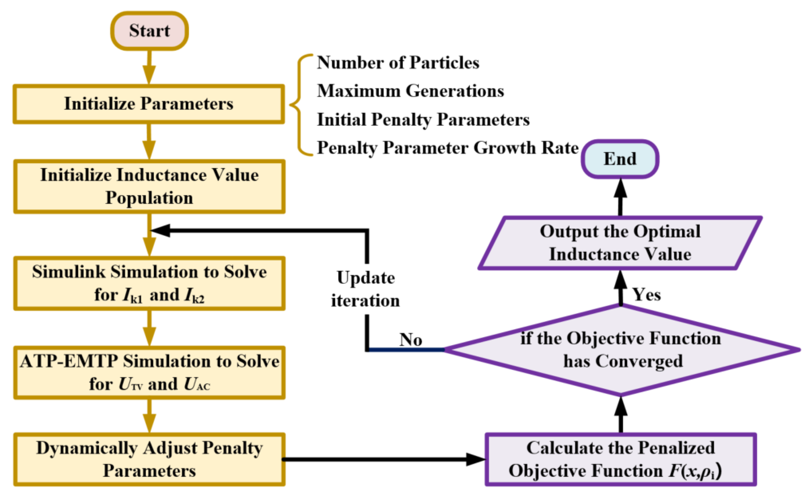
2.2.2. Objective Optimization Mode Based on the Penalty Function Method

The Penalty Function Method [19] adds a penalty term to the objective function with constraints, transforming a constrained optimization problem into an unconstrained one, thus avoiding the situation where no feasible solution can be found. In this study, the constraints, including short-circuit current and overvoltage, are converted into penalty function forms. These penalty terms are then incorporated into the objective function concerning the fault current limiter reactance value, resulting in a fitness function. This combined fitness function is used to efficiently solve the equivalent impedance value of the fault current limiter.

By introducing penalty functions k_i (i = 1, 2, 3, 4) and combining with Equations (1)–(3), the transformed conventional unconstrained optimization equation is as follows:

$$\min F(x,k_i)=f(x)+{\displaystyle \sum _{i=1}^4{k}_i\cdot max(0,g_i(x}))$$

(4)

where g_i(x) is derived from the constraint conditions as the penalty equation, as follows:

$$\left\{\begin{array}{l}{g}_1(x)=I_1(x)-\alpha I_B\\ g_2(x)=I_2(x)-\alpha I_B\\ g_3(x)=U_1(x)-v_1\\ g_4(x)=U_2(x)-v_2\end{array}\right.$$

(5)

3. Results and Discussion

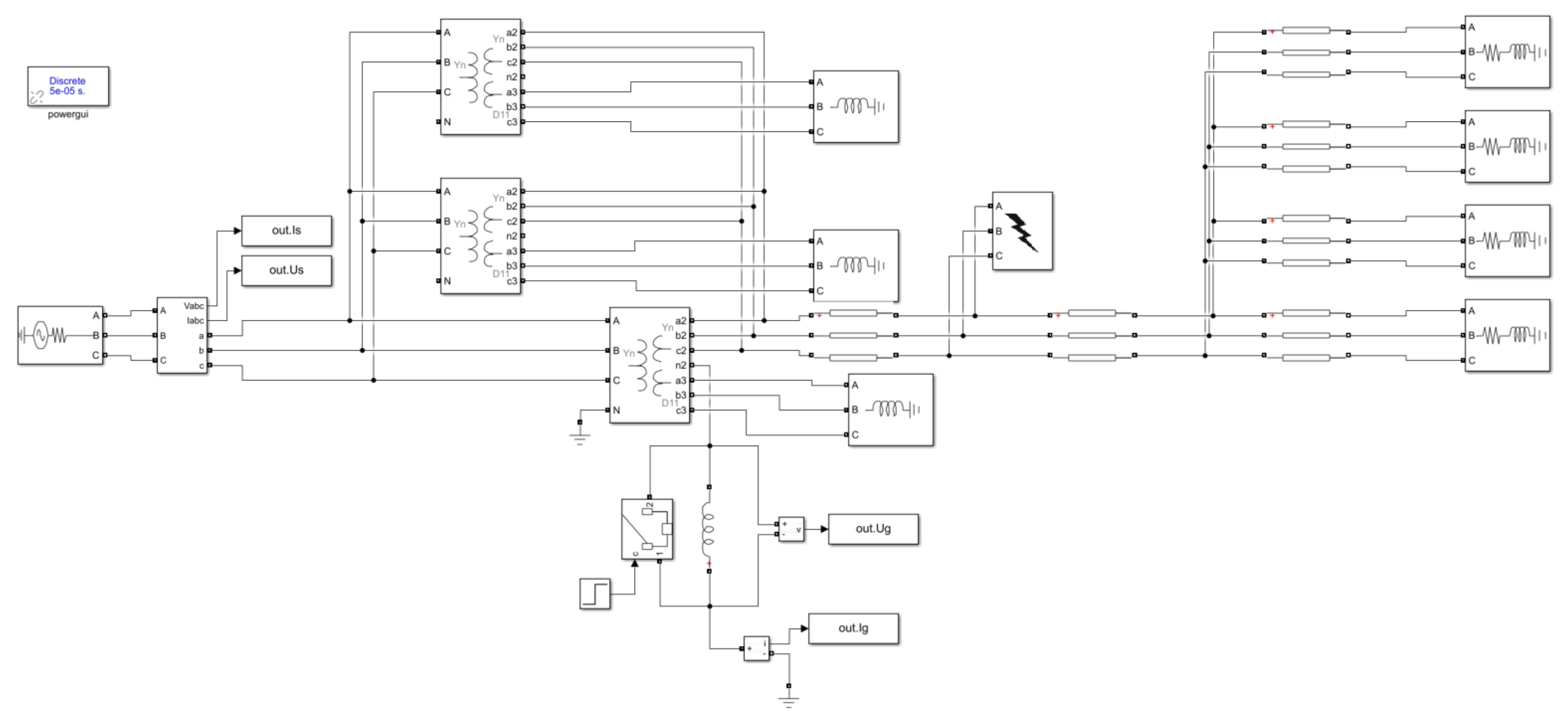
3.1. Joint Simulation Method Based on ATP and SIMULINK

In this study, both Simulink and ATP-EMTP simulation tools were utilized, as each offers distinct advantages in specific application scenarios. Simulink excels in modeling low-frequency dynamics and control systems, making it particularly suitable for analyzing power frequency components in single-phase and two-phase ground fault currents (I_k1/I_k2), where steady-state or quasi-steady-state conditions dominate. Its electrical network models enable rapid solutions and facilitate the integration of control strategies, such as the timing and logic of fast-switch actions. However, for high-frequency electromagnetic transient analysis, Simulink may introduce larger errors or require more complex models.

In contrast, ATP-EMTP is highly precise for high-frequency phenomena, such as lightning overvoltage, due to its support for smaller simulation time steps and the use of distributed parameter models for transmission lines and BCT models for transformers. This allows ATP-EMTP to better capture high-frequency transient behaviors, including neutral point overvoltage (U_TV/U_AC). Although ATP-EMTP can also analyze short-circuit currents, it is less convenient for co-simulation with control systems and other tools like MATLAB, and it demands more computational resources for high-frequency transient handling.

By combining both tools, this study achieved a comprehensive and accurate approach to address various analysis tasks. This dual-tool strategy leverages the strengths of each—ensuring high-precision electromagnetic transient analysis with ATP-EMTP and flexible control system integration with Simulink—while mitigating the limitations associated with using a single tool.

3.1.1. Simulink Short-Circuit Current Simulation Calculation

To accurately assess the severe, short-circuit faults that may occur on the medium-voltage side under the most adverse conditions, short-circuit current simulation calculations need to be carried out. The simplified system topology is shown in Figure 3. In this paper, it is assumed that the transformer and its respective system sides all operate at maximum load, and the fault location is set at the near end of the medium-voltage side of the transformer [20].

Upon analysis, it was found that installing a current-limiting reactor at the high-voltage side neutral point does not significantly increase the zero-sequence impedance at the fault point, resulting in unsatisfactory fault current limitation. Additionally, the increased impedance on the high-voltage side can cause an increase in the zero-sequence fault current flowing into the low-voltage side windings during an unbalanced ground fault, potentially creating new safety hazards. Therefore, it is advisable to install the current-limiting reactor at the medium-voltage side’s neutral point.

The simulation model built in Simulink is shown in Figure 4, where the fault type can be set at the lightning symbol position in the figure. In this model, the input is the equivalent inductance value of the fast-switching fault current limiter. When the fault type is a single-phase ground fault, the short-circuit current value I_k1 is calculated. When the fault type is a two-phase ground fault, the short-circuit current value I_k2 is calculated.

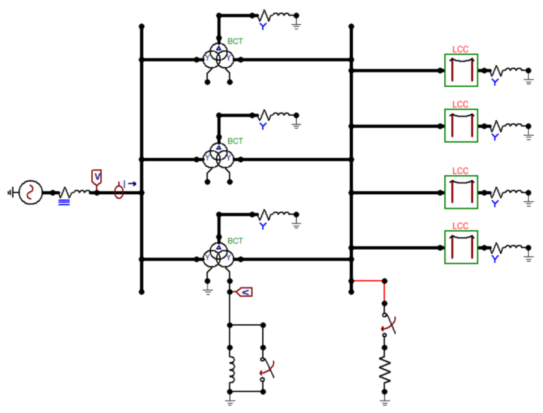
3.1.2. ATP-EMTP Overvoltage Simulation Calculation

During normal system operation, the neutral-point reactance only affects the zero-sequence loop and does not influence voltage or power flow. However, when an unbalanced short-circuit fault occurs on the line, the zero-sequence current flows through the neutral-point current-limiting reactor to the ground, which will cause the neutral-point voltage to rise [21]. If this voltage exceeds a certain threshold, it may lead to overvoltage at the transformer neutral point, surpassing the insulation withstand level, and potentially resulting in serious insulation failures. Therefore, before installing the fast-switching fault current limiter, overvoltage calculations must be performed considering the system wiring and transformer parameters to ensure the voltage remains within the insulation’s withstand range.

In this paper, ATP-EMTP simulation software (The version number of the simulationsoftware used is GNU-Mingw32 ATP) is used to model the power frequency and transient overvoltage conditions after a current-limiting reactor is installed at the neutral point of a 220 kV substation’s main transformer [22]. When building the simulation model, the surrounding power grid was simplified, and equivalent processing was applied, following the principle of maintaining power flow and node voltage unchanged to ensure the accuracy of the simulation data [23].

The simulation model is shown in Figure 5 and primarily consists of a transformer and the power grids on each side. The transformer model employs the SAT-saturated transformer model with a capacity of 120 MVA and a rated voltage of 220/121/11 kV. Both the excitation losses and short-circuit losses are set according to actual values. Three transformers operate in parallel on the high and medium-voltage sides, while the low-voltage side operates independently, with only one transformer grounded.

For the power grids on each side:

1. High-Voltage Side: The 220 kV grid is modeled using a three-phase ideal voltage source and three-phase symmetrical parallel resistors for equivalence, with a peak phase voltage of 179.6 kV.

2. Medium-Voltage Side: The 10 kV grid consists of four transmission lines with lengths of 15.93 km, 3.35 km, 8.51 km, and 31.49 km, respectively. The ends of each transmission line are modeled using three-phase symmetrical Y-connected grounding resistors as equivalent loads.

3. Low-Voltage Side: The 11 kV grid is modeled using three-phase symmetrical Y-connected grounding resistors for equivalence.

In the simulation, the fault current limiter is simplified to a current-limiting reactor. Two types of asymmetrical fault conditions are set near the medium-voltage side outlet of the transformer: one is phase A grounded through a 0.01 Ω resistor, and the other is phases B and C grounded through a 0.01 Ω resistor.

The input to this model is the equivalent reactance value of the fast-acting switch-based fault current limiter, and the outputs are the rated transient withstand voltage U₁ and the rated short-time power frequency withstand voltage U₂.

3.1.3. Joint Simulation Method of ATP-EMTP and MATLAB

To achieve joint simulation between ATP-EMTP and MATLAB, it is necessary to control the parameters in ATP-EMTP through MATLAB, modifying the model to meet the overvoltage calculation requirements under different operating conditions. Additionally, the waveform data output from ATP-EMTP calculations is saved in the “.pl4” file, which is an encrypted file, making data reading difficult.

To adjust model parameters, MATLAB’s text reading and modification functions are used to read and modify the model parameters and component states in the ATP-EMTP model configuration file.

To read the output results from ATP-EMTP, the STARTUP toolbar in the ATP-EMTP Tools toolbar is opened. In the “FMTPL4” option on the seventh tab, enter “6 × 10^13.6” to convert the encrypted “.pl4” file output by ATP-EMTP into readable decimal data.

After solving these two issues, a joint simulation between MATLAB and ATP-EMTP was achieved by calling the “.tpbig” program in MATLAB. The detailed joint simulation process is shown in Figure 6.

3.2. Gravitational Search Algorithm-Based Optimization with Joint Simulation and Comparative Analysis

3.2.1. Gravitational Search Algorithm-Based Optimization with Parameter Adaptation and Performance Comparison

However, the Penalty Function Method suffers from issues such as high computational cost and slow convergence speed [24]. Therefore, this study proposes using a GSA with adaptive dynamic adjustment of penalty parameters to avoid slow convergence caused by excessively large penalty parameters in the early stages, while ensuring effective penalization of constraint violations.

Gravitational Search Algorithm (GSA), a global optimization technique based on the law of gravity in nature, has been widely applied in various fields. As GSA has become a well-established method with numerous references available, this paper provides only a brief introduction to it [25,26,27,28].

The fundamental concept of GSA is to simulate the interaction between objects in a gravitational field to search for the optimal solution to a problem. In this algorithm, each solution is treated as an object, and the gravitational force between objects is determined by their mass and the distance between them. Larger mass objects exert a stronger gravitational pull on smaller ones, making their movement more pronounced. This allows larger objects to effectively guide smaller ones toward the global optimum.

During initialization, a set of solutions is randomly generated, with each solution’s mass proportional to its fitness. For each pair of objects i and j, the gravitational force F_ij(t) at the t-th iteration is calculated using the gravitational formula:

$$F_{ij}(t)=G{\displaystyle \frac{M_i(t)\times M_j(t)}{{R_{ij}}^2(t)}}$$

(6)

where G is the gravitational constant, M_i(t) and M_j(t) are the masses of objects i and j at the t-th iteration, and R_ij(t) is the distance between them at the same iteration. The size of the gravitational force determines the degree of attraction between the objects, thereby influencing their movement direction and speed.

During each iteration, the positions of the objects are updated according to the gravitational forces, following the update formula:

$$x_i(t+1)=x_i(t)+{\displaystyle \sum _{j=1}^N{F}_{ij}\cdot }(x_j(t)-x_i(t))$$

(7)

where x_i(t) is the position of object i at the t-th iteration, and x_j(t) is the position of object j. The gravitational force F_ij between objects i and j affects their movement toward each other. The parameter N denotes the number of particles in the population. With each iteration, the objects gradually move toward the optimal solution. As the iteration count increases, the gravitational force decreases, causing the objects’ velocities to reduce until they converge to the optimal solution or meet the stopping criterion.

To validate the superiority of GSA over conventional optimization methods in FCL reactance configuration, we conducted comparative analyses with Genetic Algorithm (GA) and Particle Swarm Optimization (PSO) under two scenarios.

1. Single Reactance Optimization

Based on the practical validation provided in the case study in Section 3.3, which focuses on the Hebei power grid, a comparative analysis of the GSA, GA, and PSO was conducted. Using the example of a FCL installed at the neutral point of a 220 kV transformer, the following parameter settings were applied: for the PSO algorithm, the inertia weight is set to 0.6, and the learning factors are set as c1 = 1.7 and c2 = 1.5 [29]; for the GA, the crossover probability is set to 0.8, and the mutation probability is set to 0.1 [30]. The comparison results are summarized in the

Table 1. Comparison of the Convergence Performance of Different Optimization Methods.

Algorithm	Average Convergence Iterations	Optimal Solution x (mH)	Solution Std. Dev σ (mH)	Computation Time (s)
GSA	83	15.9	<0.01	948.1
GA	33	15.9	<0.01	363.7
PSO	134	15.9	<0.01	1436.8

.

The results show that in the optimization of a single current-limiting reactance value, the convergence rate follows GA > GSA > PSO, with all three algorithms stably converging to the same optimal solution (15.9 mH) and a standard deviation below 0.01 mH. Additionally, the results indicate that computation time is primarily influenced by the number of iterations, as each algorithm iteration takes less than 0.1 s, while the simulation step for each iteration exceeds 10 s. Although GA exhibits the fastest convergence, practical applications prioritize robust global search capabilities to ensure stable identification of the global optimal solution. In real-world engineering scenarios, where multiple FSFCLs are installed at various points, the optimization of reactance values evolves into a multimodal problem with numerous local optima, making GSA’s global search advantage critically important.

2. Multi-Reactance Optimization

Consider the following scenario: three FSFCLs are installed at the neutral points of a 220 kV substation, and one FSFCL is installed on each of five feeder lines. The objective function in this case can be simply set as:

$$\min f={\displaystyle \sum _{j=1}^8{\lambda }_j}{x}_j$$

(8)

where x_j represents the current-limiting reactance value of each FSFCL, and λ_j represents the influence weight of each reactance value. In this scenario, the weights λ_j are assumed to be set as 1, 0.5, 2, 1, 1.5, 2, 1, and 0.5, respectively.

The constraints are assumed to remain unchanged. At this point, different combinations of reactance values may lead to similar objective function values, meaning the objective function has multiple local optima. After running the program for 100 iterations, the results are summarized in

Table 2. The Global Optimal Solution Hit Rate of Different Optimization Methods.

Algorithm	Global Optimal Solution Hit Rate
GSA	92%
GA	78%
PSO	67%

.

Through the above simple case, it can be observed that the GSA demonstrates superior global search capabilities compared to the other two methods, making it more suitable for practical engineering applications in the optimization and selection of current-limiting reactance values.

3.2.2. Gravitational Search Algorithm Key Parameter Settings

The main advantage of GSA lies in its strong global search capability, which helps in preventing entrapment in local optima. This feature makes it especially suitable for high-dimensional, complex optimization problems. By utilizing gravitational interactions between objects, GSA promotes comprehensive exploration of the solution space and demonstrates excellent convergence and optimization performance.

To further enhance the application of GSA in optimizing FCL reactance configurations, several key parameters are carefully designed as follows:

1. GSA Parameter Design

(1) Gravitational Constant Evolution

The gravitational constant G is dynamically adjusted using an exponential decay function to balance exploration and exploitation:

$$G\left(t\right)=G_0\cdot e^{{-\alpha (t/T)}^{\beta }}$$

(9)

where β = 0.7; G₀ = 100, and α = 20, are empirical coefficients derived from power grid optimization studies [31].

(2) Initialization Strategy

1) Position Initialization

Adopting the asymmetric sampling method from [32]:

$$x_i(0)=x_{\min }+\left[{\left(rand+0.1i\right)}^{1.5}\right]\cdot \left(x_{\max }-x_{\min }\right)$$

(10)

2) Mass Initialization

Fuzzy-transformed fitness values characterize object masses:

$$M_i(0)={\displaystyle \frac{\exp (-F_i/\sigma )}{{\displaystyle {\sum }_{j=1}^N\exp (-F_j/\sigma )}}}$$

(11)

where F_i represents the fitness value of the i-th object, σ is the standard deviation of the fitness values (used to normalize the distribution), and N is the population size.

3) Velocity Initialization:

Initial velocities v_i(0) = 0 minimize early-stage divergence risks.

(3) Population Parameters

1) Population Size

The population size N is as follows [33]:

$$N\ge 10\cdot n$$

(12)

where n is the problem dimension (n = 1 in this study).

However, considering practical application scenarios where the selection of current-limiting reactance values for multiple FSFCLs may be required, the number of devices typically does not exceed ten. Taking into account convergence efficiency, solution accuracy, and computational cost, a population size of N = 100 was ultimately chosen.

2) Maximum Iterations

Based on the convergence analysis in [34], the maximum number of iterations, D, should meet the following condition:

$$P(D)\ge 99.8\%$$

(13)

where P(D) denotes the probability of convergence within D iterations.

During the actual iterative computation process, the iteration count required for solution convergence occasionally exceeds 100. Therefore, the maximum number of iterations is set to 200 in this study to ensure a sufficient convergence probability while maintaining a certain margin.

During the iterations, the penalty factor is dynamically adjusted based on the current constraint violations. The penalty factor in this study is initially set to 1 and increases proportionally with each iteration, intensifying the penalty for constraint violations. This dynamic adjustment mechanism ensures that the algorithm prioritizes solutions that satisfy the constraints throughout the search process, guiding the algorithm toward feasible solutions.

When the objective function value changes very little over several iterations and satisfies the convergence criteria, it indicates that the algorithm has found a solution close to the optimal one. At this point, the algorithm can be terminated. Through this iterative process, the optimal reactance value for the fault current limiter (FCL) is determined.

The selection of Δk = 1.1 in this study is based on the dynamic adjustment theory [24], which employs a linearly increasing penalty coefficient to prevent insufficient constraint weighting during the early iterations. This incremental strategy has been validated as effective in the IEEE CEC 2017 benchmark tests.

In addition to the penalty factor’s incremental adjustment, the selection of the initial penalty parameter k_n0 requires careful consideration. A balance must be achieved between its impact on constraint satisfaction and convergence performance. If k_n0 is set too small, the algorithm may fail to adequately penalize constraint violations, leading to unacceptable errors. Conversely, if k_n0 is set too large, it may increase computational complexity and reduce algorithm efficiency. Therefore, the selection of k_n0 must be approached with caution in practical applications.

For the computational scenario in this study, both current and voltage constraints are critical. Violating these constraints would lead to unacceptable outcomes, making it essential to set k_n0 sufficiently large to strictly enforce the constraints while avoiding overly small values. To evaluate the impact of different initial penalty parameter values, in the context of the case study in Section 3.3 of this paper, an analysis was conducted using k_n0 values of 0.001, 0.01, 0.1, 1, 10, and 100. The results of this analysis are shown in

Table 3. Comparison of convergence performance under different k_n0 values.

kn0	Average Convergence Iterations	Optimal Solution x (mH)
0.001	82	8.9
0.01	83	14.1
0.1	83	15.7
1	83	15.9
10	82	15.9
100	83	15.9

.

As shown in Table 3, all parameter settings achieve convergence with nearly identical convergence iterations. However, when k_n0 is relatively small (e.g., 0.001 or 0.01), the resulting optimal reactance value fails to meet the constraint conditions and shows significant deviation from the expected value. As k_n0 increases, the optimization results gradually stabilize, and the constraints are strictly satisfied.

Considering both convergence accuracy and computational efficiency, this study selects k_n0 = 1 as the initial penalty parameter. This value ensures that the constraints are strictly enforced while maintaining computational efficiency and solution accuracy.

The overall calculation process proposed in this paper is shown in Figure 7.

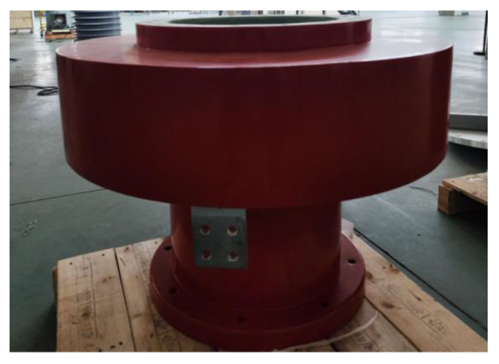
3.3. Case Study Analysis

This paper takes the No. 1 main transformer of a 220 kV substation in the Hebei power grid as an example to analyze the situation of asymmetric short circuits occurring on the medium-voltage side of the transformer. The high-voltage side of the transformer is independently powered, and the high- and medium-voltage sides operate in parallel with two other transformers that have nearly identical parameters, while the low-voltage side operates independently.

The basic parameters of the transformer are as follows: rated voltage of 220/121/11 kV, rated capacity of 120/120/60 MVA, short-circuit impedance of 14.1%, 24.0%, and 7.32%, connection group YNyn0D11, and the transformer core is a three-phase five-column type.

The current-limiting target for the windings on each side of the transformer is set to 1.94/2.85/17.90 kA.

Using the optimization configuration method proposed in this paper, the optimal inductance value calculated is 15.9 mH. The variation and convergence process of the current-limiting reactance values obtained through iterations is shown in Figure 8.

Based on the convergence curve, the current-limiting reactor value shows significant oscillations during the first 20 iterations, ranging from approximately 16 mH to 30 mH, indicating that the GSA is still in the global search phase and has not yet converged. Between the 20th and 45th iterations, the oscillations decrease, and the reactor value gradually stabilizes around 16mH, reflecting partial convergence. From the 50th iteration onward, the reactor value becomes increasingly stable, achieving full convergence near the 80th iteration and locating a region close to the optimal solution.

At this reactance value, the short-circuit current values for each winding under different fault conditions, as well as the maximum transient overvoltage and maximum power frequency steady-state overvoltage at the neutral point of the medium-voltage side, are presented in

Table 4. Calculation Results under Various Fault Conditions.

Fault Conditions	High-Voltage Side Winding Current (kA)	Medium-Voltage Side Winding Current (kA)	Low-Voltage Side Winding Current (kA)
Single-phase ground fault	0.92	2.78	7.05
Two-phase ground fault	1.80	2.85	4.54

.

In both fault scenarios, the current-limiting targets are achieved, and the short-circuit current constraints are met. Additionally, the maximum transient overvoltage on the medium-voltage side neutral point is 74.6 kV, and the maximum power–frequency steady-state overvoltage is 49.8 kV. Both values are lower than the insulation level of the 110 kV side neutral point equipment, thus satisfying the overvoltage constraint requirements.

Based on the comprehensive analysis presented above, this paper ultimately ascertains the optimal limiting reactance value for the equipment to be 15.9 mH. A corresponding fault current limiter has been fabricated accordingly. The subsequent step entails preparing for commissioning and field application. The specific physical prototype is depicted in the Figure 9 and Figure 10.

4. Conclusions

This paper proposes a novel optimization method for FSFCL reactance configuration based on joint simulation and penalty function constraint optimization. By integrating MATLAB and ATP-EMTP for joint simulation, the method effectively derives the constraint conditions of the objective optimization function, providing critical data support for the optimization process. To address the challenges of high computational complexity and solution difficulties in constrained optimization problems, the PFM is employed to transform the constrained optimization problem into a standard unconstrained optimization problem, significantly reducing computational complexity and ensuring solution feasibility. Subsequently, the GSA is applied to compute the optimal reactance value. Through a comparative analysis based on engineering case studies, the superiority of the GSA over GA and PSO is validated, further confirming the accuracy and efficiency of the proposed method. The results demonstrate that the method not only achieves precise parameter calculations but also significantly enhances computational efficiency. By combining PFM and GSA, the proposed approach exhibits excellent robustness, providing reliable technical support for the application and deployment of fast-switching fault current limiters in large-scale power grids.

References

1. Yu, Y.; Wei, M.; Lyu, P.; Yang, G.; Wang, C. A practical modeling method for new energy stations applicable to asymmetric fault short-circuit calculation. Power Grid Technol. 2024, 48, 4788–4795. [Google Scholar]
2. Liu, Y. Analysis and treatment of low-voltage short-circuit faults in 220 kV main transformers. Hebei Electr. Power Technol. 2017, 36, 53–55. [Google Scholar]
3. Zheng, S.; Liu, H.; Zhu, S. Two-step optimization method for limiting measures of three-phase and single-phase short circuits. Electr. Meas. Instrum. 2019, 56, 70–75+81. [Google Scholar]
4. Han, B.; Chen, W.; Chang, N.; Jin, Y.; Qie, X.; Han, Y.; Zhu, B.; Tan, S.; Yu, Y.; Zhang, J.; et al. Research on short-circuit current limitation method based on system topology dynamic adjustment. Grid Technol. 2021, 45, 1158–1166. [Google Scholar]
5. Zhao, E.; Han, Y.; Liu, Y.; Zalhaf, A.S.; Wang, C.; Yang, P. Feasibility analysis of neutral grounding by small reactor of HVDC converter transformer. Energy Rep. 2022, 8 (Suppl. S1), 392–399. [Google Scholar] [CrossRef]
6. Chen, T.; Li, B.; Han, Y.; Li, Q.; Wang, J.; Jin, J. Research on fault line selection of small current grounding system considering zero sequence unbalanced current. Electr. Porcelain Light. Arrester 2022, 124–130. [Google Scholar]
7. Liu, J.; Yuan, J.; Zhou, H.; Li, X.; Mo, Z. Parameter design of short-circuit fault limiter considering the transient component of short-circuit current in high-voltage AC systems. High Volt. Technol. 2024, 50, 3769–3785. [Google Scholar]
8. Wang, W.; Zhao, Y.; Xu, Y.; Lv, W.; Yang, B.; Fang, T. Canister-type rapid switch for 500 kV fast switching fault current limiter. High Volt. Technol. 2023, 49, 803–811. [Google Scholar] [CrossRef]
9. Im, I.G.; Choi, H.S.; Jung, B.I. Limiting characteristics of the superconducting fault current limiter applied to the neutral line of conventional transformer. Phys. C Supercond. 2013, 494, 339–343. [Google Scholar] [CrossRef]
10. Sahebi, A.; Samet, H. Discrimination between internal fault and magnetizing inrush currents of power transformers in the presence of a superconducting fault current limiter applied to the neutral point. IET Sci. Meas. Technol. 2016, 10, 537–544. [Google Scholar] [CrossRef]
11. Gong, X.; Gao, C.; Long, Z.; Lin, Y.; Xu, L. Principle of asymmetric short-circuit current limitation by adding a small reactance at the neutral point of 500kV auto-transformer. Electr. Power Constr. 2013, 34, 56–60. [Google Scholar]
12. Xu, M. Research on Modeling and Application of Complex High Coupling Split Reactor for Fault Current Limiter. Master’s Thesis, Huazhong University of Science and Technology, Wuhan, China, 2020. [Google Scholar]
13. Han, N.; Jia, X.; Zhao, X.; Xu, J.; Zhao, C. A new topology of hybrid DC fault current limiter. Proc. Chin. Soc. Electr. Eng. 2019, 39, 1647–1658+1861. [Google Scholar]
14. Hong, J.; Guan, Y.; Xu, G. Selection of fault current limiter installation position and parameter calculation in large power grids. High Volt. Appar. 2010, 46, 62–66. [Google Scholar]
15. Hu, J.; Li, X.; Yang, Y.; Bao, X.; Li, J. Analysis of neutral grounding overvoltage of 220 kV transformer. Electr. Porcelain Light. Arrester 2019, 152–158. [Google Scholar]
16. Xu, D. Research on Fault Current Limiter Based on Fast Switch. Master’s Thesis, Dalian University of Technology, Dalian, China, 2021. [Google Scholar]
17. Q/GDW169-2008; Oil-immersed Transformers (Reactors) Condition Evaluation Guide. State Grid Corporation of China: Beijing, China, 2008.
18. GB 311.1-2012; Insulation Coordination Part 1: Definitions, Principles and Rules. Standardization Administration of China: Beijing, China, 2012.
19. Jia, L.; Li, W.; Zhao, C. Numerical optimization design of vehicle cooling fan based on penalty function method. Mech. Des. Manuf. 2020, 201–205+210. [Google Scholar]
20. Zhang, B.; Zhang, W.; Guo, S.; Wang, X.; Li, T. Simulation calculation of transformer differential current containing non-periodic components in external short circuits. Hebei Electr. Power Technol. 2023, 42, 82–85+94. [Google Scholar]
21. Zhao, H.; Zhang, X.; Cao, W.; Cheng, Z.; Gao, S. Study on overvoltage protection of ultra-high voltage transformer neutral point grounded through a small reactance. Insul. Surge Arresters 2022, 109–115. [Google Scholar]
22. Zhang, W.; Ding, Q.; Hu, G.; Qiao, Z.; Ma, X. Research on lightning overvoltage protection scheme of distribution transformer based on ATP-EMTP simulation analysis. Electr. Porcelain Light. Arrester 2020, 86–92. [Google Scholar]
23. Kang, S.; Feng, W.; Qin, Z.; Jia, H. Overvoltage analysis of fast power supply restoration for transformers with ungrounded neutral points after faults. Hebei Electr. Power Technol. 2019, 38, 5–8. [Google Scholar]
24. Si, C.; Lan, T.; Hu, J.; Wang, L.; Wu, Q. Discussion on the penalty coefficient in the penalty function. Control. Decis. 2014, 29, 1707–1710. [Google Scholar]
25. Aditya, N.; Mahapatra, S.S. An adaptive gravitational search algorithm for optimizing mechanical engineering design and machining problems. Eng. Appl. Artif. Intell. 2024, 138, 109298. [Google Scholar] [CrossRef]
26. Roy, A.; Verma, V.; Gampa, S.R.; Bansal, R.C. Planning of distribution system considering residential rooftop photovoltaic systems, distributed generations and shunt capacitors using gravitational search algorithm. Comput. Electr. Eng. 2023, 111, 108960. [Google Scholar] [CrossRef]
27. Shukla, A.; Momoh, J.A. Pseudo inspired gravitational search algorithm for optimal sizing of grid with integrated renewable energy and energy storage. J. Energy Storage 2021, 38, 102565. [Google Scholar] [CrossRef]
28. Omkar, S.; Arabinda, G.; Kumar, A.R. Estimation of parameters of one-diode and two-diode photovoltaic models: A chaotic gravitational search algorithm-based approach. Energy Sources Part A Recovery Util. Environ. Eff. 2023, 45, 5938–5956. [Google Scholar]
29. Marini, F.; Walczak, B. Particle swarm optimization (PSO): A tutorial. Chemom. Intell. Lab. Syst. 2015, 149, 153–165. [Google Scholar] [CrossRef]
30. Coello, C.A. An updated survey of GA-based multiobjective optimization techniques. ACM Comput. Surv. (CSUR) 2000, 32, 109–143. [Google Scholar] [CrossRef]
31. Zhang, X.; Liu, B.; Wang, Y. Day-ahead reactive power optimization scheduling strategy for active distribution networks considering operating condition prediction errors. J. North China Electr. Power Univ. (Nat. Sci. Ed.) 2024, 51, 31–40. [Google Scholar]
32. Rashedi, E.; Nezamabadi-Pour, H.; Saryazdi, S. GSA: A gravitational search algorithm. Inf. Sci. 2009, 179, 2232–2248. [Google Scholar] [CrossRef]
33. Sareni, B.; Krahenbuhl, L. Fitness sharing and niching methods revisited. IEEE Trans. Evol. Comput. 1998, 2, 97–106. [Google Scholar] [CrossRef]
34. Deb, K.; Agrawal, R. Simulated binary crossover for continuous search space. Complex Syst. 1995, 9, 115–148. [Google Scholar]
Figure 1. Schematic diagram of FSFCL structure.
Energies 18 01077 g001
Figure 2. The physical model diagram of FSFCL.
Energies 18 01077 g002
Figure 3. Power system topology diagram of a 220 kV substation.
Energies 18 01077 g003
Figure 4. Simulink asymmetric short-circuit simulation model.
Energies 18 01077 g004
Figure 5. Simulation Circuit of a 220 kV Substation Power System.
Energies 18 01077 g005
Figure 6. ATP-EMTP and MATLAB Joint Simulation Flowchart.
Energies 18 01077 g006
Figure 7. Flowchart for Adaptive Dynamic Adjustment of Penalty Parameters and Solution of Objective Function.
Energies 18 01077 g007
Figure 8. Convergence Curve of the Objective Function Using the GSA.
Energies 18 01077 g008
Figure 9. Photograph of the current-limiting reactor.
Energies 18 01077 g009
Figure 10. Overall physical image of the fault current limiter.
Energies 18 01077 g010