Optimal Allocation and Sizing of BESS in a Distribution Network with High PV Production Using NSGA-II and LP Optimization Methods

Abstract

Battery energy storage systems (BESSs) can play a significant role in overcoming the challenges in Distribution Systems (DSs) with a high level of penetration from renewable energy sources (RESs). In this paper, the goal is to determine the optimal location, size, and charging/discharging dispatches of BESSs in DSs with a high level of photovoltaic (PV) installations. The problem of the location and size of BESSs is solved with multi-criteria optimization using Non-dominated Sorting Genetic Algorithm-II (NSGA-II). The criteria of the multi-criteria optimization are minimal investment costs for BESS and improvement of the network performance index. The network performance index includes the reduction in annual losses of active energy in DSs and the minimization of voltage deviations. The dispatch of a BESS is determined using auxiliary optimization. Linear Programming (LP) is used for auxiliary optimization, with the aim of dispatching the BESS to smooth the load profile in DS. The proposed optimization method differs from previous studies because it takes in its calculations all days of the year. This was performed using the K-means clustering technique. The days of one year are classified by the level of consumption and PV production. The optimization was performed for five different levels of PV penetration (60%, 70%, 80%, 90%, and 100%) and for two scenarios: the first with one BESS and the second with two BESSs. The proposed methodology is applied to the IEEE 33 bus balanced radial distribution system. The results demonstrate that with an optimal choice of location and parameters of the BESS, significant improvement in network performance is achieved. This refers to a reduction in losses of active power, improvement of voltage profile, smoothing the load diagram, and reducing the peak load. For the scenario with one BESS and PV penetration of 100%, the reduction in daily energy losses reaches a value of up to 10% compared to the base case (case without a BESS). The reduction in peak load goes to 20%. Further, the highest voltage during the day is significantly lower in all buses compared to the base case. Similarly, the lowest voltage during the day is considerably higher. The methodology from this paper can be applied to any radial distribution network with a variable number of BESSs. The testing results confirm the effectiveness of the proposed method.

1. Introduction

Today, electricity generation must always be balanced with the load. Balancing load and generation is a critical aspect of power grid operation. This has become less predictable in recent years, with more RESs being connected to the grid. With the increasing role of variable generation and changing demand profiles, grid operators have limited resources to maintain this dynamic balance.

BESSs can help grid operators maintain the dynamic balance in systems with high penetration of variable RESs. In DSs with high PV penetration and no BESS, network security may be compromised. The potential problems include high voltages in the buses, overloaded branches of the network, reverse power flows, etc. It is in the interest of the distribution system operator (DSO) to avoid such situations. One of the possible solutions is the installation of a BESS. A BESS can significantly enhance the efficiency, stability, and resilience of electricity networks. A BESS can provide a number of benefits to the distribution network [1], typically categorized based on the time scale. The following factors must be considered to efficiently and economically install a new BESS in the DS: the optimal location and the optimal size of the BESS. If a BESS is suitably deployed, it can give the grid operators a flexible and fast-responding resource to manage variability in generation and load effectively. From the standpoint of the DSO, finding the optimal BESS number, as well as its location and capacity, is a critical issue that has been tackled over the last few years. Many studies have explored the optimal location and size of BESSs to improve various problems in the network caused by the high penetration of RESs.

Different optimization techniques were used for these purposes. Papers [2,3,4] investigate using BESSs to improve voltage regulation problems in both DS and microgrids—the authors use modified NSGA-II in [2], binary grey wolf optimization in [3], and the power sensitivity matrix in [4].

Papers [5,6,7,8,9,10] deal with loss reduction and total system energy reduction with the help of BESS. The authors in [5] propose using a metaheuristic rider optimization algorithm. Reference [6] introduces a modified Henry gas solubility optimization algorithm. Paper [7] presents a two-layered optimization, which includes African buffalo optimization and heuristic optimization. Reference [8] applies the Archimedes optimization algorithm. The whale optimization algorithm appears in [9], while [10] uses both the genetic algorithm (GA) and Particle Swarm Optimization (PSO). The study in [11] aims to reduce energy losses and CO₂ emissions by integrating BESSs. It combines two technologies: a parallel discrete version of the vortex search algorithm and PSO.

Regarding energy arbitrage as an objective, [12] proposes a robust and efficient planning-operation methodology using a non-linear programming model for solving the optimal integration of BESSs and distributed generation (DG).

The literature mentioned above considers only one criterion for improving the network’s condition. Some papers investigate more than one criterion for solving problems in DSs using BESSs. In [13], the authors present a methodology for the determination of the size of both the PV DG and BESS by a multi-objective nested optimization framework. The goal is to minimize annual energy losses, feeder power loss, reverse power flow, load deviation index, and node voltage deviation and maximize the BESS utilization index. Reference [14] describes the determination of the optimal location and size of BESS along with its charging and discharging schedules. The objective is to minimize voltage violations and line overloading. The methods include PSO, novel bat, firefly, coyote, and krill herd optimization. The authors in [15] present a methodology for BESS location in DS, with an objective function that combines various benefits of BESS. These benefits are energy arbitrage, energy loss reduction, lower BESS investment costs, reduced transmission access fees, and decreased environmental emissions. They use a GA. Reference [16] investigates how the location and capacity of BESS affect voltage fluctuations and power losses in a DS with DG, applying an improved NSGA-II. Paper [17] demonstrates using a multi-objective evolutionary algorithm based on decomposition to solve DS problems by combining the DG and BESS. The analysis includes reducing power losses, minimizing energy not supplied, cutting load costs, and reducing voltage deviations. In [18], the location and size of the BESS are determined using NSGA-II to decrease losses and improve voltage stability in DS.

There are also papers on which the minimization of the costs of the DSO is the objective of optimization. To minimize the daily costs of the DS caused by voltage regulation, power losses, and peak demand by finding the optimal location and size of the BESS, authors in [19] suggest using PSO, while those in [20] recommend both GA and PSO. Three optimization algorithms (GA, PSO, and salp swarm algorithm) are compared in [21] for finding the optimal location and size of the BESS in terms of power loss costs, peak power demand costs, and voltage regulation costs. In [22], the optimization problem is to find the optimal size of BESS in a microgrid to minimize the investment costs of the BESS and operational costs of the microgrid. The algorithm combines quadratic programming with binary PSO. In [23], the authors optimize the location and size of the BESS to reduce the DS cost incurred from purchasing energy within one day using artificial ecosystem optimization. In [24], using multi-objective equilibrium optimization, the authors seek the optimal location and size of DG and BESSs. The aim is to reduce the operation and investment costs of both BESS and DG, the cost of power losses, the cost of energy not supplied, and the cost of CO₂ emissions. In [25], the authors apply mixed integer linear programming to reduce the microgrid’s operational and investment costs by finding the optimal size of the DG and BESS.

As the literature shows, one of the most crucial issues during the implementation of BESSs is optimally determining the tradeoff between the investment costs of BESS and the economic and technical benefit that DSO obtains from using BESS. The literature study [26] lists comprehensive reviews of BESS sizing criteria, methods, and applications in various renewable energy systems.

In all cited papers, the optimal location and parameters of the BESS were determined using only one daily profile (consumption profile and PV production profile). This profile represents either an average daily profile or a profile corresponding to some critical day. The present study differs because all days of the year are subject to optimization. In this way, the variability of consumption and PV production is modeled, which is not possible with a model with only one daily profile.

This paper presents a methodology for determining the optimal location and parameters (energy and capacity) of BESSs in medium voltage DSs with high PV penetration. The study assumes that the DSO owns the BESS. The idea is to find the optimal location and parameters of the BESS to improve the performance of the distribution network while taking care of the investment costs of BESS. The performance of the distribution network is measured by the network performance index. The network performance index includes two network indicators: reduction in annual losses of active energy in DS and minimization of voltage deviations. The two criterion functions model the problem. The first function presents BESS costs, while the second presents the network performance index. These two criterion functions are optimized simultaneously. The NSGA-II method, which is commonly used for multi-criteria optimization, was chosen to solve this optimization problem.

In addition to NSGA-II, auxiliary optimization is applied for the determination of optimal BESS dispatching with the objective to “smoot” the consumption profile. LP is used for auxiliary optimization. Smoothing the consumption profile improves network performance. A measure of smoothing the consumption profile is the network performance index.

The consumption and PV production profiles are variables that differ daily. For one year, these data have significant seasonal and daily oscillations. When using only one selected day (an average day or the most critical day of the year), the result of optimization may not apply to other days. To obtain the results from the optimization that are realistic and applicable for every day of the year, in this paper, all days of the year are considered while searching for the optimal location, size, and daily operation of the BESS. This was performed using the K-means clustering technique [27].

Hence, the problem that authors consider in this paper can be formulated along these lines: the goal is to find the location and parameters of a BESS, considering all days of the year, to optimize the network performance index and the investment costs of BESS.

Taking into consideration those mentioned above, the main contributions of this paper are summarized as follows:

• A proposed optimization method takes into consideration all days in one year. This was performed using the K-means clustering technique. The days of one year are classified by the level of consumption and the level of PV production. The clusters are obtained by combining groups of days with similar levels of PV production and consumption. The number of clusters is input data for optimization, and it is changeable;
• Simultaneous optimization of two key indicators of the distribution network using a network performance index. The goal of the criterion function modeled in this way is that the decision-maker when applying this method to a real network, chooses which key indicators of the distribution network will be optimized. Each indicator has a weighting factor, whose value is between 0 and 1. Selecting the value for weighting factors allows the decision-maker to prioritize some of the key indicators of the distribution network. For each key indicator, it is possible to choose its influence on the optimization process;
• Smoothing the fluctuations of the load profile. This could help the DSO to optimally dispatch the BESS based on the load and PV production forecast;
• Determination of the initial value of the energy in the BESS by optimization;
• Using the combination of NSGA-II and LP algorithms, which proved to be effective and not time-consuming for solving this kind of problem in distribution networks;
• Developing an original program in MATLAB 2024a to implement the described methodology. The advantage of the developed program is that it can be adapted to the different needs of the user and to any radial distribution network with a variable number of BESS.

The optimization results in a set of solutions, from which the decision maker (the DSO) selects the final solution.

The remainder of the paper is organized into four sections. Section 2 presents the proposed optimization model. Section 3 provides numerical results obtained through the proposed methodology. The discussion appears in Section 4, and Section 5 concludes the paper.

2. Proposed Optimization Model

This section presents the proposed optimization model. The problem of finding optimal location and BESS parameters in this paper is a multi-criteria problem. These two criterion functions, which are simultaneously optimized, model this problem. The first criterion function determines BESS investment costs, while the second criterion function determines the network performance index. The optimization aims to find the optimal location and parameters of the BESS in the DS to improve the performance of the distribution network while taking care of the investment costs of BESS.

The investment costs of BESSs are calculated as follows:

$$f_1=C_P{P}_{B,rated}+C_E{E}_{B,rated},$$

(1)

where C_P is the cost per W, C_E is the cost per Wh, P_B,rated is the power rating, and E_B,rated is the rated energy capacity. The network performance index is calculated as follows:

$$f_2={\displaystyle \frac{{\omega }_1{I}_1+{\omega }_2{I}_2}{{\omega }_1+{\omega }_2}},$$

(2)

where I₁ and I₂ are performance indicators and ω₁ and ω₂ are weighting factors for I₁ and I₂. Indicator I₁ represents the relative ratio of the voltage deviation in the distribution network, which is calculated using Equations (3)–(5):

$${\sigma }_d=\sqrt{{\displaystyle \frac{1}{24}}{\displaystyle \sum _{t=1}^{24}{\displaystyle \sum _{k=1}^{N_n}{(U_{tk}-U_{ref})}^2}}}, d=1, 2, \dots , D,$$

(3)

$${\sigma }_y=\sqrt{{\displaystyle \frac{1}{365}}{\displaystyle \sum _{d=1}^D{N}_d{\sigma }_d^2}},$$

(4)

$$I_1={\displaystyle \frac{{\sigma }_y^{BESS}}{{\sigma }_y^{BASE}}},$$

(5)

where U_tk is the voltage module in bus k at hour t for cluster d, U_ref is the reference value of voltage, N_n is the number of buses in the distribution network, σ_d is voltage deviation for cluster d, D is number of clusters, N_d is number of days in cluster d, σ_y is annual voltage deviation in distribution network, σ_y^BESS is annual voltage deviation in distribution system with BESS and σ_y^BASE is annual voltage deviation in distribution system without BESS (base state of distribution network). Indicator I₂ represents the relative ratio of yearly losses of active energy in the distribution network, calculated using Equations (6)–(8):

$$W_d={\displaystyle \sum _{t=1}^{24}{P}_t}\cdot 1h, d=1, 2, \dots , D,$$

(6)

$$W_y={\displaystyle \sum _{d=1}^D{N}_d{W}_d},$$

(7)

$$I_2={\displaystyle \frac{W_y^{BESS}}{W_y^{BASE}}},$$

(8)

where P_t represents losses of active power in the distribution network at hour t for cluster d, N_d is the number of days in cluster d; W_d represents losses of active energy in the distribution network for cluster d, W_y are annual losses of active energy in the distribution network, W_y^BESS are annual losses of active energy in the distribution network with a BESS and W_y^BASE are annual losses of active energy in the distribution network without a BESS (base state of distribution network).

I₁ and I₂ formulated in this way compose a common network performance index, which is subject to optimization. The weighting factors ω₁ and ω₂ for performance indicators I₁ and I₂, respectively, are input values for calculation. Their value is between zero and one. If the weighting factor for the performance indicator is equal to zero, that performance indicator is not subject to optimization. On the other hand, if both weighting factors are equal, both performance indicators have the same importance in optimization. In this way, choosing values for the weighting factors makes it possible to provide a greater impact on one performance indicator over the other. The optimization results are optimal for the selected combination of the weighting factors. The results are expected to differ for a different combination of the weighting factors. In this case, the decision maker, DSO, determines the weighting factors for every optimization process. Following its business plans and current problems in the network, DSO chooses which performance indicator to optimize by selecting values for the weighting factors.

Considering all the above-mentioned functions, the optimization problem could be defined as follows:

$$\min (f_1,f_2).$$

(9)

The NSGA-II algorithm [28,29] was applied to solve the optimization problem. NSGA-II is a standard algorithm for solving multi-criteria optimization problems. In the problem posed, the criterion functions f₁ and f₂ are simultaneously optimized using this algorithm.

NSGA-II is a population-based evolutionary algorithm. In this optimization problem, the population consists of chromosomes whose structure is shown in Figure 1.

The meaning of individual values from Figure 1 are:

• Loc—the bus where BESSs will be installed;
• P_B,rated—the power rating;
• E_B,rated—the rated energy capacity;
• E₀—the energy level in BESS at the beginning of the day.

These values represent the control variables in the optimization process.

The optimization begins with forming an initial population P with a given number of chromosomes. Each chromosome contains information about the location and parameters of the BESS and represents a potential solution to the optimization problem. Every possible solution (chromosome) should ensure that a BESS will improve network performance. For this purpose, auxiliary optimization was applied to every potential solution. Auxiliary optimization aims to determine the optimal BESS dispatching that will enhance the network’s performance.

It is necessary to define the following values to describe the auxiliary optimization:

• Pd_t—total active power demand in the distribution network in hour t;
• Ps_t—total PV production in the distribution network in hour t;
• Pc_t—charging/discharging power of BESS in hour t;
• P_t—deviation of load from the average daily load;
• P_avg—an average daily load value in the distribution network before installation of BESS.

The average daily value of load in the distribution network before installation of BESS is calculated as follows:

$$P_{avg}={\displaystyle \frac{{\displaystyle \sum _{t=1}^{24}(P{d}_t-P{s}_t)}}{24}}.$$

(10)

For every hour h in cluster d, the deviation of load from the average daily load (P_t) is calculated as follows:

$$P_t=(P{d}_t-P{s}_t)-P_{avg}.$$

(11)

The main intention of the auxiliary optimization is the “smoothing” of the load diagram. A BESS should operate so that the load diagram is as close as possible to the average daily load. Taking this into consideration, the criterion function could be described as follows:

$$\min {\displaystyle \sum _{t=1}^{24}\left|P_t+P{c}_t\right|}.$$

(12)

The BESS is discharged during the hours when P_t has a positive value, and the BESS is charged during the hours when P_t has a negative value. The BESS is not charged or discharged in hours where P_t is equal to zero. This could be described as follows:

$$\begin{array}{l}{P}_t>0 \Rightarrow P{c}_t<0\\ P_t<0 \Rightarrow P{c}_t>0\\ P_t=0 \Rightarrow P{c}_t=0\end{array}.$$

(13)

The mathematical model of the BESS and the operational limitations are described by Equations (14)–(17). When Pc_t is positive, the BESS is charged and when Pc_t is negative, the BESS is discharged. While tackling this optimization problem, there are also some constraints that must be satisfied. These constraints are related to the capacity and energy of the BESS. Charging and discharging processes could be described as follows:

$$E_{t+1}=\left\{\begin{array}{c}{E}_t+P{c}_t\cdot {\eta }_c, P{c}_t>0\\ E_t+P{c}_t/{\eta }_d, P{c}_t<0\end{array}\right.,$$

(14)

where E_t is energy in the BESS at the end of hour t, E_t+1 is energy in the BESS at the beginning of hour t + 1, η_c and η_d are charging and discharging efficiency, respectively. The following constraints must be satisfied in every hour:

$$E_t^{\min }<E_t<E_t^{\max },$$

(15)

where E_t^min and E_t^max are the minimum and maximum energy of the BESS, respectively. In hours in which the BESS is charging (Pc_t > 0), the following constraint must be satisfied:

$$0<P{c}_t<P{c}^{C\max }.$$

(16)

In hours in which the BESS is discharging (Pc_t < 0), the following constraint must be satisfied:

$$-P{c}^{D\max }<P{c}_t<0.$$

(17)

Pc^Cmax and Pc^Dmax are the maximum charging and discharging power rates, respectively. In addition to the constraints mentioned above, some limitations ensure that BESS load diagrams before and after the charging/discharging process stay on the same side of the P_avg line. These constraints eliminate the absolute value from the criterion function in (12). Because it is already known in which hours the value P_t + Pc_t is greater than zero and in which hours the value P_t + Pc_t is lower than zero, the criterion function should be described as follows:

$$\min \left\{{\displaystyle \sum _{t\in T_D}(P_t+P{c}_t)-{\displaystyle \sum _{t\in T_C}(P_t+P{c}_t)}}\right\}.$$

(18)

T_D is the set of hours in which the BESS is discharging, and T_C is the set of hours in which the BESS is charging. An optimization problem described in this way and with given constraints can be efficiently solved using LP. The result of the auxiliary optimization is the charging/discharging power of the BESS, as well as the level of energy in the BESS for every hour of the individual cluster.

For every chromosome of the initial population P, the optimal dispatch of the BESS is calculated using the auxiliary optimization. This is performed for all clusters. Then, for every chromosome and every cluster, the network state is calculated. For the calculation of the state of the network, the Shirmohammadi method [30], also known as the backward/forward algorithm, is used. This is a standard method for calculating power flows in a radial distribution network. Based on the network state, the criteria function f₂ is calculated using Equations (2)–(8). The criteria function f₁ is calculated based on values from the chromosome (values for P_B,rated and E_B,rated). In this way, the values of the criterion functions f₁ and f₂ were determined for all chromosomes in the initial population.

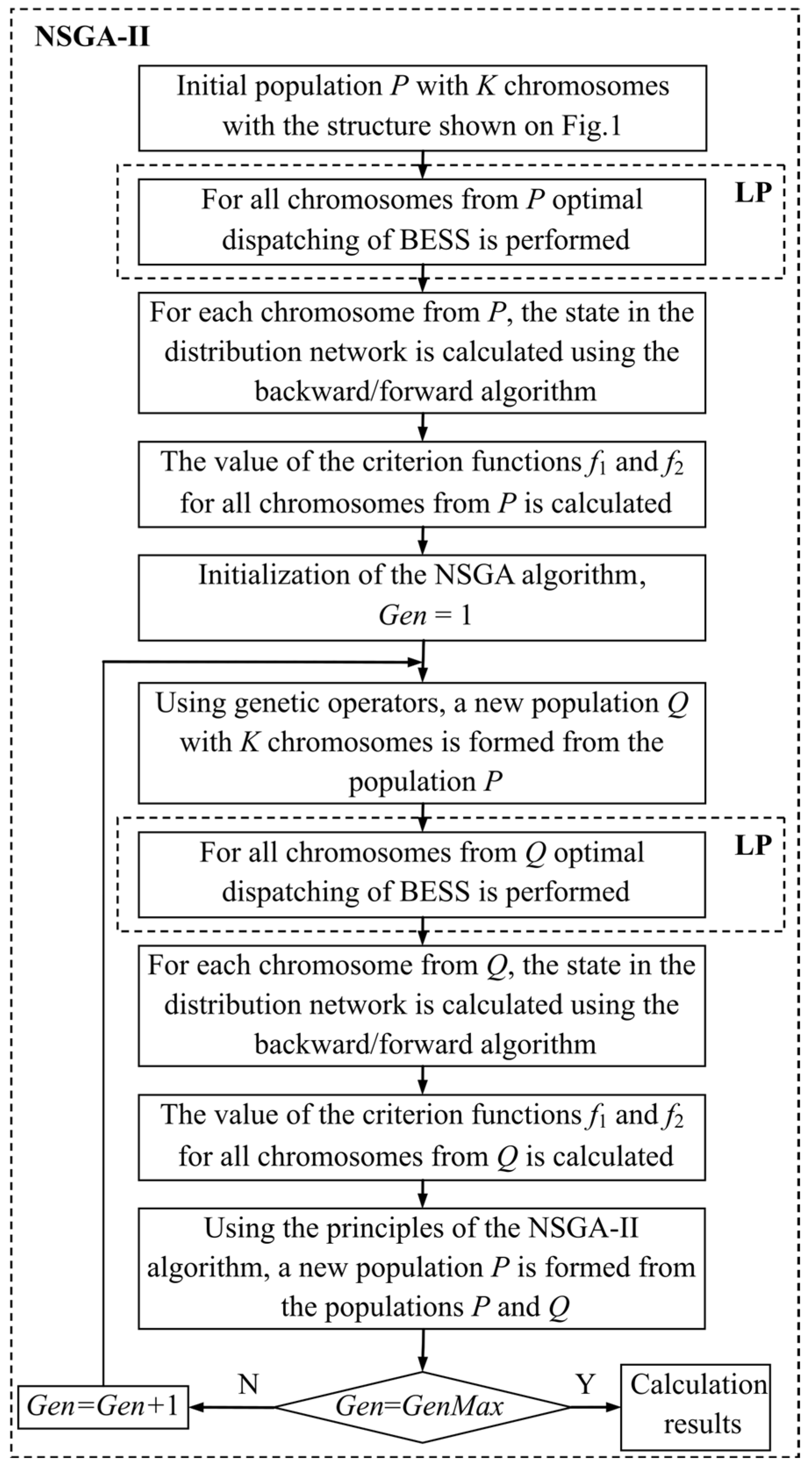
A new population, Q, is formed by applying genetic operators (selection, crossover, and mutation) to the initial population, P. A “roulette wheel” was used for the selection, a one-point crossover with an 80% probability was used for the crossover, and mutation applies in the standard way for binary coding with a 5% probability. For every chromosome of population Q, all steps for population P are performed—auxiliary optimization, calculation of the state of the network, and calculation of the criterion functions f₁ and f₂. Then, by combining populations P and Q using non-dominated sorting principles of NSGA-II, a new population P is formed, which starts a new generation. The procedure is repeated for the given number of generations. In every new generation, the criterion functions f₁ and f₂ have better values than those of the previous generation.

The model presented in this paper could be applied to any radial distribution network with a variable number of BESSs. The complete flow of the optimization process is presented in Figure 2.

As a result of the multi-criteria optimization, the set of optimal solutions or Pareto optimal solutions is obtained [28,29]. According to the principles of Pareto optimality, the obtained solutions represent a compromise between two criterion functions, f₁ and f₂.

In addition to the BESS operating constraints, all solutions must satisfy the operational constraints of the distribution network. One of these constraints is the balance of active and reactive power in all buses of the distribution network. These constraints are satisfied by calculating the network state using the backward/forward algorithm. The other restrictions are listed below.

Values of voltage must be within the defined limits for every solution:

$$U_{\min }\le U_{tk}\le U_{\max },$$

(19)

where U_min and U_max are the maximum and minimum voltage values at bus k, respectively, and U_tk is the voltage magnitude at bus k at hour t. Further, power flows in branches must be within the defined limits:

$$\left|{\underset{¯}{S}}_{tk}\right|\le S_k^{\max },$$

(20)

where S_tk is the apparent power in branch k at hour t, and S_k^max is the maximum allowable power in branch k.

Every solution must also satisfy the constraints regarding the reverse power flows. It is necessary to limit reverse power flows to avoid energy flows from the distribution network to the transmission network. The following equitation can describe this constraint:

$${\theta }_{1,t}>{\theta }_{2,t}$$

(21)

where θ_1,t and θ_2,t are voltage angles at buses 1 and 2 at hour t.

If the optimization gives a solution that does not satisfy one of the set constraints, that solution is eliminated from the optimization process. Therefore, the obtained set of optimal solutions satisfies all the set constraints. The obtained set of optimal solutions represents the best approximation of the real Pareto front for this optimization problem.

3. Case Studies and Results

This section presents the network used to test the proposed methodology, and the results obtained by applying the methodology. The proposed methodology is applied to the IEEE 33 bus balanced radial distribution system [31], shown in Figure 3. The IEEE 33 system is a standard test system and has been used as a test grid in many works dealing with the optimal location of the BESS [2,5,7,13,14,15,16,20,21,23].

Table 1. Network parameters and the maximum transmission capacity of the branches.

Bus i	Bus j	R [p.u.]	X [p.u.]	B [p.u.]	Smax [p.u.]
1	2	0.0058	0.0029	0	0.5
2	3	0.0308	0.0157	0	0.4
3	4	0.0228	0.0116	0	0.3
4	5	0.0238	0.0121	0	0.3
5	6	0.0511	0.0441	0	0.3
6	7	0.0117	0.0386	0	0.2
7	8	0.0444	0.0147	0	0.2
8	9	0.0643	0.0462	0	0.2
9	10	0.0651	0.0462	0	0.2
10	11	0.0123	0.0041	0	0.2
11	12	0.0234	0.0077	0	0.2
12	13	0.0916	0.0721	0	0.2
13	14	0.0338	0.0445	0	0.2
14	15	0.0369	0.0328	0	0.2
15	16	0.0466	0.0340	0	0.2
16	17	0.0804	0.1074	0	0.2
17	18	0.0457	0.0358	0	0.2
2	19	0.0102	0.0098	0	0.2
19	20	0.0939	0.0846	0	0.2
20	21	0.0256	0.0298	0	0.2
21	22	0.0442	0.0585	0	0.2
3	23	0.0282	0.0192	0	0.3
23	24	0.056	0.0442	0	0.3
24	25	0.0559	0.0437	0	0.3
6	26	0.0127	0.0065	0	0.2
26	27	0.0177	0.0090	0	0.2
27	28	0.0661	0.0583	0	0.2
28	29	0.0502	0.0437	0	0.2
29	30	0.0317	0.0161	0	0.2
30	31	0.0608	0.0601	0	0.2
31	32	0.0194	0.0226	0	0.2
32	33	0.0213	0.0331	0	0.2

provides data on network parameters and the maximum transmission capacity of the branches.

Table 2. Active and reactive power in individual buses of the network.

Bus i	P [p.u.]	Q [p.u.]	Bus i	P [p.u.]	Q [p.u.]	Bus i	P [p.u.]	Q [p.u.]
1	0	0	12	0.006	0.0035	23	0.009	0.005
2	0.010	0.006	13	0.006	0.0035	24	0.042	0.020
3	0.009	0.004	14	0.012	0.008	25	0.042	0.020
4	0.012	0.008	15	0.006	0.001	26	0.006	0.0025
5	0.006	0.003	16	0.006	0.002	27	0.006	0.0025
6	0.006	0.002	17	0.006	0.002	28	0.006	0.002
7	0.020	0.010	18	0.009	0.004	29	0.012	0.007
8	0.020	0.010	19	0.009	0.004	30	0.020	0.060
9	0.006	0.002	20	0.009	0.004	31	0.015	0.007
10	0.006	0.002	21	0.009	0.004	32	0.021	0.010
11	0.0045	0.003	22	0.009	0.004	33	0.006	0.004

contains data on active and reactive power in individual network buses. All data are given in [p.u.] according to base values U_b = 12.66 kV and S_b = 10 MVA.

The DSO in Serbia provided the data for consumption profiles. The data for PV production profiles came from measuring solar irradiation in the Southern Banat region of Serbia (Supplementary Materials Table S1). This is a region with very good potential for producing electricity from the sun. The IEEE 33 network is of medium voltage. It was assumed that many consumers are connected to each network bus. There is no consumption on bus 1. It is assumed that there is PV production in each bus of the network. Each bus is represented by a daily profile of consumption and PV production.

Based on these data, all days of the year were grouped into clusters using the K-means clustering technique [27]. This widely used technique partitions a set of data into K clusters, minimizing the sum of the squared distances between the data and their assigned cluster mean. The number of clusters is an input value of calculation, and it can be adapted. In this paper, the number of clusters equals nine. This is performed as follows: 365 daily consumption profiles are classified into three groups depending on the consumption level- low, medium, and high consumption level. In the same way, 365 daily profiles of PV production of the same year are depending on the production level, grouped into three groups—low, medium, and high PV production levels. Using crosscheck, all 365 days of the year were identified to which group of consumption level and PV production level they belong. Then, combining three groups of consumption and three groups of production, nine clusters were obtained. In this way, all days of one year were classified into nine clusters presented in Figure 4. Figure 4 shows the normalized profiles of consumption and PV production for the entire network. The PV production profiles and consumption profiles for individual buses are obtained by scaling the profile from Figure 4. The degree of PV penetration and consumption in individual buses from Table 1 and Table 2 are used for scaling.

In Figure 4, the first row represents all days with low consumption: Cluster 1 represents all days with low consumption and low PV production, Cluster 2 represents all days with low consumption and medium PV production, and Cluster 3 represents all days with low consumption and high PV production. The second row represents all days with medium consumption: Cluster 4 represents all days with medium consumption, and so on. Finally, Cluster 9 represents all days with high consumption and PV production. Figure 4 also presents an overview of the number of days of the year belonging to each cluster.

The optimization was, therefore, performed for nine clusters, considering the number of such days in a year, to include all days of the year in the calculation. In this way, the variable character of consumption and PV production for one year is modeled in the calculation.

The level of PV penetration was calculated as a percentage of the maximum load in buses. The optimization was performed for five different levels of PV penetration—60%, 70%, 80%, 90%, and 100%. The degree of PV penetration is assumed to be the same across all buses in the distribution network. All buses except bus 1 can be targeted for the BESS location. The voltage on bus 1 is 1.05 p.u. while the voltages on all other buses are limited from 0.95 p.u. to 1.05 p.u. It is assumed that the shapes of both load profiles and PV production profiles are identical in all buses, but profiles are scaled according to IEEE 33 system data [31].

The minimum level of energy (E_min) in the BESS during the day is limited to 10% of E_B,rated while the maximum level of energy (E_max) is limited to 90% of E_B,rated. With these limitations, the BESS’s operational life is prolonged. The initial value of the energy in the BESS (E₀) is determined by optimization and its minimum is limited to 10% of E_max, and its maximum is limited to 50% of E_max.

Regarding the energy management of the BESS, the level of energy of BESS should reach its initial value at the end of the day. The efficiency coefficient for both the charging and discharging states is 0.9. The number of charging and discharging cycles is not limited to one during the day. E_B,rated and P_B,rated are control variables, and they are determined by optimization. For both scenarios and for all PV penetration levels, E_B,rated can have a value from the range of 0 MWh to 10 MWh, while P_B,rated can have a value from the range of 0 MW to 2 MW. The costs C_P and C_E, which figure in criterion function f₁, are 0.18 €/W and 0.43 €/Wh, respectively. The weighting factors ω₁ and ω₂ for criterion functions f₁ and f₂ are equal to 1.

The authors have developed an original program in MATLAB 2024a for applying the described methodology. The methodology can be applied to any radial distribution network where the number of BESSs can vary (one, two, or more). This paper examines two scenarios. The first scenario considers the installation of one BESS, and the second considers the installation of two BESSs. In both scenarios, calculations were made for five different levels of PV penetration. For each level of PV penetration, the calculation includes 200 generations with a population of 40 chromosomes. Each calculation results in a set of optimal solutions. Figure 5 shows the results for the first scenario for five different levels of PV penetration. Figure 6 presents the results for the second scenario for the same five levels of PV penetration.

The results obtained represent a set of optimal solutions for two scenarios. These results represent a set of compromise solutions for two criteria functions, f₁ and f₂ (investment costs and network performance index), optimized simultaneously, considering all constraints. The set of optimal solutions shows how network performance depends on investments in BESS. In almost every optimization problem, one or more constraints are dominant, and they determine the optimal solution. The results for these two scenarios showed that the reverse power flow constraints have a dominant effect on the set of optimal solutions. Therefore, the sets of optimal solutions from Figure 5 and Figure 6 are limited on the left side by the constraint on reverse power flows. The first solutions in the set of optimal solutions for every penetration level (solutions marked with A, B, C, D, and E in Figure 5 and Figure 6) correspond to the minimum investment in BESSs. These solutions indicate the minimum investments to avoid reverse power flows in the distribution network. For the level of penetration of 60%, in both scenarios, one compromise solution has the value of the criterion function f₁ equal to 0 and the value of the criterion function f₂ equal to 1 (point marked with A in Figure 5 and Figure 6). This solution shows that with the level of 60% PV penetration in the network, reverse power flows do not occur. Therefore, one of the optimal solutions is not to install the BESSs in the distribution network. Since optimization gives such a solution as one of the possible ones, it proves the robustness of the applied NSGA-II method.

Table 3. Selected solutions for the scenario with 1 BESS.

Sol.	Location	PB,rated [MW]	EB,rated [MWh]	E0 [×Emax]	f1 [103 €]	f2
A	-	0	0	-	0	1
B	16	0.084	0.899	0.204	401.84	0.9931
C	26	0.391	3.754	0.163	1692.55	0.9824
D	6	0.751	6.334	0.117	2858.89	0.9732
E	6	1.079	8.367	0.402	3792.30	0.9639

presents the results for solutions A, B, C, D, and E from Figure 5, and

Table 4. Selected solutions for the scenario with 2 BESS.

Sol.	Location	PB,rated [MW]	EB,rated [MWh]	E0 [×Emax]	f1 [103 €]	f2
A	-	0	0	-	0	1
	-	0	0	-
B	17	0.064	0.645	0.114	453.04	0.9925
	30	0.094	0.342	0.203
C	6	0.524	3.763	0.115	1773.24	0.9812
	18	0.056	0.117	0.186
D	6	0.843	5.347	0.499	2750.57	0.974
	24	0.1	0.655	0.313
E	6	1.017	6.031	0.106	3921.41	0.9616
	24	0.313	2.532	0.249

shows the results for solutions A, B, C, D, and E from Figure 6.

Some buses appear dominantly as a solution to the optimization problem for the BESS location. In the first scenario, which is bus 6, while in the second scenario, buses 6 and 24. In the literature [20,21,23], bus 6 also appears most often as the optimal location for the BESS.

For some solutions, the initial value for E₀ is close to the minimum (10% of E_max), while other solutions have a significantly higher initial value. These are solutions B and E for the scenario with one BESS and solution D for the scenario with two BESSs. This shows that it is better to optimize the value of E₀ rather than set a value for E₀ as an input parameter, as performed in [2,3,5,7,9,12]. BESS does not have to be discharged to the minimum value at the beginning of each day but to the value obtained through optimization. This approach enables energy savings.

In both scenarios, the decision on which solution to choose from the set of solutions ultimately depends on the decision-maker (in this case, the DSO). The DSO selects a solution based on criteria aligned with its business decisions. These criteria can be financial or technical performance, or both requirements together, or others.

An analysis of the solutions for both scenarios indicates that installing two BESSs does not significantly improve network performance.

Therefore, further analysis will focus only on the results from the first scenario (one BESS). A case with a PV penetration level of 100% has been selected.

For this case, Figure 7 presents the final optimization solution E (the same as in Figure 5), along with the initial population used at the start of the optimization. This figure clearly shows how much optimization helps in finding the optimal solution. The solutions from the initial population can be interpreted as the solutions that someone would propose without knowing the characteristics of the distribution network and the profile of consumption and PV production. Optimization can significantly help decision-makers avoid such wrong conclusions.

Since an evolutionary optimization method such as NSGA-II does not guarantee obtaining an accurate Pareto front, the authors performed a new calculation to verify the proposed method. Instead of the NSGA-II method for multi-criteria optimization, the Multi-Objective Particle Swarm Optimization method (MOPSO) [32] was used for the simultaneous optimization of two criterion functions. In this case, LP was also used as auxiliary optimization to determine the optimal dispatching of BESS. LP is a very efficient method that guarantees the achievement of convergence for a given criterion function and constraints.

Figure 8 presents a comparative view of the optimal solutions obtained using two different multi-criteria optimization methods: NSGA-II and MOPSO. The same scenario was used for comparison: one BESS and a PV penetration level of 100%. Although these two methods apply different principles to find optimal solutions, the results largely coincide. Because of that, it can be concluded that the proposed method resulted in a set of optimal solutions that is a good approximation of the true Pareto front. However, with NSGA-II methods, the solutions spread better along the Pareto front.

The solution with the minimum investment costs will undergo a detailed analysis. This is solution E in Figure 5, Figure 7, and Table 3. This solution was selected to show the impact of BESS on network performance. The authors selected cluster number 3 (low consumption, high PV production) for this analysis because this is the most critical cluster from the aspect of the distribution network, and it represents most days of the year.

Figure 9 shows the load profile of the network before and after BESS installation for the selected case. It can clearly be seen to what extent the load profile is smoothed using BESS. The peak load before the installation of BESS was 2.163 MW, and after installation, it was 1.718 MW, which is a decrease of 20.6%. This significant shift in peak load can delay planned investments in distribution capacities. In addition, using BESS eliminates the reverse power flows, which appear in hours where PV penetration is high and consumption is low. From the aspect of the distribution network, eliminating reverse power flows is a very significant result.

Figure 10 shows a diagram of the voltage profiles before and after installing the BESS for the selected case. The profiles show the hours with the lowest and highest voltages. These results demonstrate the improvement in the voltage profile across all buses after installing the BESS.

Figure 11 shows a diagram of active energy losses in the distribution network before and after the installation of BESS. Daily energy losses are 0.711 MWh without BESS and 0.643 MWh with BESS, which is a reduction of 9.6%. It is important to emphasize that in terms of active energy losses, optimization is performed on a daily basis. It could happen that losses are lower in the case without BESS in some hours during the day (in Figure 11, this happens in hours 2–8). However, the total daily losses of active energy are significantly lower in the case of BESS installation. These results are important because they indicate daily loss reduction, although there are additional losses of energy because of BESS operation (charging and discharging).

In addition to optimal siting and sizing of the BESS, proper operation of the BESS is also important to be considered. Figure 12 shows the charging and discharging power of the BESS in each hour for the selected solution (solution E). As expected, the BESS charges during periods of high PV production. It discharges at the end of the day to ensure the energy level at the day’s end matches the initial energy value from the start of the day. Figure 13 shows the energy levels for the BESS throughout the day for the selected solution.

The optimization process determines the optimal dispatching for each cluster. Therefore, the charging and discharging periods of the BESS are not always the same. The BESS control model depends on the consumption level and PV production level every hour for individual clusters.

4. Discussion

This section analyzes the results from the case study and the proposed methodology. The presented model has the advantage of being easily adaptable to different user needs.

The user can choose the level of PV penetration for the calculation. Calculations, which include different levels of penetration, can be used for network development planning due to new renewable sources, considering an expected increase in PV penetration. Additionally, when the only goal is to avoid reverse power flows, the results of calculations may indicate the level of PV penetration at which installing BESSs is unnecessary. This paper shows that for applied networks, this level is 60% of PV penetration. At this level of PV penetration, the results show that there is no reverse power flow.

One of the criterion functions (function f₂) in the presented model is the network performance index, which is a function of two network indicators. One indicator refers to the voltage profile, and the other refers to active energy losses. The user can choose whether to optimize with only one or both indicators. Further, by assigning values to the weighting factors, the user can give greater importance to one of the indicators during optimization. The choice of all these parameters depends on the user’s needs and whether there is a specific problem in the distribution network that BESS installation could solve. The criterion function f₂ could expand with some additional indicators in case of further development of the proposed method.

BESS cost and efficiency are input parameters of the calculation that affect the optimization results. The calculation will yield different solutions depending on these parameters.

The problem described in this paper is related to the distribution network development and planning domain. When solving planning problems, calculation time does not play a key role in evaluating the effectiveness of the method. Therefore, it is not necessary to perform calculations in real time and very fast. However, even though this problem is not real-time but a planning problem, it is essential to emphasize that the calculation took about 30 min. This is the time of the calculation for one scenario (the scenario with one BESS or the scenario with two BESSs) with the selected level of PV penetration. The calculation time is not long, considering that the NSGA-II algorithm could be very time-consuming. The calculation time of NSGA-II depends on the choice of input parameters. The input parameters of the calculation are quite demanding (200 generations, with a population of 40 chromosomes). Further, for every 200 generations, an auxiliary optimization was performed using LP, where the parameters of BESS are calculated, and the state of the network is calculated (using the backward/forward algorithm) considering all constraints. The calculations ran on a computer with an i7 processor and 16 GB RAM. Since the calculation process is not time-consuming, the proposed model can easily apply to real distribution networks of higher dimensions with more than one or two BESS. This could help DSOs in network development and planning processes.

Many papers determine the optimal location, power, and energy of the BESS using one daily consumption profile and a PV production profile. The profiles used in those papers represent either some average daily profile or a profile corresponding to some critical day. In the author’s opinion, such an approach cannot cover all days of the year since every day has different combinations of daily consumption profiles and PV production profiles. For this reason, the authors apply the K-means clustering technique to include all days of the year in the calculation. This process includes classifying all days of the year into clusters, each representing a set of days based on daily consumption and PV production profiles. The authors deem that this is a significant contribution because it directly implies that the results (location and parameters of BESSs) obtained in this way are more precise. They fit all days of the year, not only one day, and consequently, they have a better impact on the smoothing of the diagram and improvement of the network performance.

The authors performed an additional calculation highlighting the advantages of using the K-means clustering technique. Additional calculations compare the K-means clustering technique with the consumption and PV production profiles corresponding to an average day. The authors obtained the average consumption profile and PV production profile by averaging values for all days of the year. The first scenario (one BESS) and level of PV penetration of 80% serve for the analysis. Figure 14 shows the results by using the K-means clustering technique and using profiles of an average day. The results differ significantly. When using an average day, it may happen that some critical days of the year, from the aspect of set constraints, are not registered due to averaging. Using the K-means clustering technique, some of the clusters consider all critical days, and it cannot happen that some of the constraints are violated. It can be seen from Figure 14 (and Figure 7) that the set of optimal solutions obtained using the K-means clustering technique has a limit on the left side. The reason for this is all the constraints set. On the other hand, this is not the case for the results obtained using an average day. Figure 14 presents a solution where the value of the criterion function f₁ equals zero. This could lead to the conclusion that, at the chosen level of PV penetration, there is no violation of the constraints, and therefore, it is unnecessary to install BESS. Still, as was shown in the previous sections, this is a wrong conclusion.

The number of clusters is one of the calculation parameters and can be changed. Optimization of this number was not the subject of this work. In this work, the number of clusters is nine. Increasing the number of clusters would increase the calculation time, while not significantly different results would be obtained as with nine clusters. With nine clusters, daily variations in consumption and PV production can be modeled to a good extent without too long a calculation time.

5. Conclusions

This section provides a conclusion and the author’s intentions for future work. This paper presents the method for optimal sitting and sizing of BESS in a distribution network with high PV penetration. The following were used: NSGA-II and LP optimization methods, the K-means clustering technique, and different levels of PV penetration.

The proposed method shows that the selection of the optimal location and size of the BESS, as well as its optimal dispatching, can significantly improve network performance. Installing a BESS can improve the voltage profile, reduce daily active power losses, and smoothen the network load profile. For the case study presented in this paper in Section 3, the reduction in daily energy losses is 0.068 MWh (9.6%) compared to the base case (without BESS). The reduction in peak load is 0.445 MW (20.6%). Regarding voltage profiles, the results show that high voltages are significantly lower in all buses of the distribution network compared to the base case. Analogously, low voltages are significantly higher. In addition, the reverse power flows, which occur in distribution networks with a high PV penetration, can be prevented. The K-means clustering technique was used to classify the days of a year, and this method included all days of the year. This approach produced a more realistic result than the calculation where optimization focuses on only one day (average or some critical day). As a result of the optimization, a set of optimal solutions was obtained. A decision maker, in this case, the DSO, chooses a solution that corresponds to its technical and economic criteria, which are of interest. The optimization uses a combination of NSGA-II and LP algorithms. NSGA-II is a standard method for multi-criteria optimization problems. LP, used to optimize BESS dispatching, has proven to be fast and effective. Both optimization methods demonstrated their advantages in finding the optimal solution. In conclusion, this methodology can be used for efficient planning of the development of any radial distribution networks that face uncertainties caused by the increasing number of RES. Users can adjust some input calculation parameters, such as the number of BESSs, the level of PV penetration, the number of clusters, and the weighting factors for key indicators, to suit the specific situation.

The variability of load and PV production is modeled with nine clusters. However, the stochastic nature of consumption and PV production, which can affect optimization results, is not fully modeled in this way. Additionally, the paper did not model BESS aging and efficiency degradation, negatively impacting BESS performance. They have a negative effect on the work of BESS. To include these two characteristics in the calculation, it would be necessary to perform optimization for every year of the BESS lifetime and to predict when to replace BESS. In future works on this topic, the authors plan to include these phenomena in the BESS model as well as the stochastic nature of load and PV production. Further, in future work on this topic, optimization of the coordinated work of BESS and charging stations in urban transportation can be considered. This topic is relevant in cities with developed transport electrification [33].