Abstract
To overcome the incomplete decomposition of vibration signals in traditional motor-bearing fault diagnosis algorithms and improve the ability to characterize fault characteristics and anti-interference, a diagnostic strategy combining dual signal reconstruction and deep learning architecture is proposed. In this study, an improved complete ensemble empirical mode decomposition with adaptive noise (CEEMDAN) and variational mode decomposition (VMD)-based signal reconstruction method is first introduced to extract features representing motor bearing faults. A feature matrix construction method based on improved information entropy is then proposed to quantify these fault features. Finally, a fault diagnosis algorithm architecture integrating a multi-scale convolutional neural network (MSCNN) with attention mechanisms and a bidirectional long short-term memory network (BiLSTM) is developed. The experimental results for four fault states show that this model can effectively extract fault features from original vibration signals and, compared to other fault diagnosis models, offer high diagnostic accuracy and strong generalization, maintaining high accuracy even under varying speeds and noise interference.
1. Introduction
Electric motors are ubiquitous in the realm of rotating machinery and find extensive application across electrical and energy-related industries. However, their operation often occurs under harsh conditions, making them prone to failures that can lead to shutdowns and pose significant threats to production safety. To ensure safe and continuous operations while mitigating economic losses associated with maintenance and repair, rapid and accurate fault diagnosis of motor bearings is essential [1,2].
Traditionally, fault diagnosis methods for electric motor bearings have relied on signal processing techniques [3,4,5]. These methods typically analyze vibration signals or current signals in the time domain, frequency domain, or both, to diagnose bearing faults. Commonly used signal processing methods include empirical mode decomposition (EMD) [6], variational mode decomposition (VMD) [7], and wavelet transform [8]. While EMD is capable of processing non-linear and non-stationary signals using adaptive basis functions, it may suffer from mode mixing, which can degrade the accuracy of signal decomposition [9]. Ensemble empirical mode decomposition (EEMD) addresses this issue by effectively suppressing mode mixing [10]. VMD, as a newer adaptive signal processing method, transforms the signal decomposition process into a variational problem, thereby achieving adaptive separation of signals without mode mixing or endpoint effects [11,12]. Despite these advancements, the non-stationary and non-linear characteristics of real-world bearing vibration signals present challenges for feature extraction. As a result, traditional signal processing approaches alone make it hard to provide adaptive fault diagnosis. The development of fault classification methods integrating multiple methodologies has become a leading direction in this field.
With the advent of artificial intelligence, deep neural networks have demonstrated unique advantages in handling data with non-linear relationships. Numerous studies have applied deep learning algorithms to establish mappings between signals and faults, facilitating fault diagnosis for electric motor bearings [13]. The limitations of traditional CNNs have led to the emergence of a new type of CNN called CapsNet, which overcomes the problems of CNN position information loss and feature reuse [14]. Additionally, Ref. [15] indicated that traditional deep learning-based bearing fault diagnosis methods assume that the training and testing data follow the same distribution. However, in practical scenarios, the distribution of bearing data may vary, invalidating this assumption and leading to a significant decline in diagnostic performance. To address this issue, the concept of transfer learning has been introduced in deep learning, allowing knowledge gained from other data or models to be transferred to the current task, thereby effectively resolving this problem. Similarly, algorithm architectures based on combined recurrent networks have also been proposed to overcome similar problems. For instance, a combined Convolutional Neural Network (CNN) and Long Short-Term Memory (LSTM) model was proposed for bearing fault diagnosis [16] using time–frequency images and vibration signals as inputs for multi-dimensional feature extraction and fusion. Another study introduced a hybrid CNN-LSTM neural network for end-to-end rolling bearing fault diagnosis [17]. Yet another approach combined the CNN and bidirectional LSTM (BiLSTM) to adaptively extract features for bearing fault diagnosis [18]. Although these integrated methods have shown promise, they still face challenges in complex vibration environments, including incomplete signal decomposition, weak correlation between defect features and signals, and limitations in model interpretability and generalization.
To address these issues, we propose a novel fault diagnosis model based on signal reconstruction and feature dependency. In our research, we first combine Improved Complete Ensemble Empirical Mode Decomposition with Adaptive Noise (ICEEMDAN) and VMD to extract effective vibration signal components under complex noise conditions. We then introduce an improved signal entropy-based method to quantify defect features, yielding parameters corresponding to different fault states. Finally, we utilize attention mechanisms to enhance the interpretability and generalization capabilities of the MSCNN-MSBiLSTM model for fault diagnosis. Our results demonstrate that the proposed model can adaptively adjust its parameters based on signal features, achieving a diagnostic accuracy of 95% under laboratory conditions. Thus, the methodology presented here offers a new algorithmic framework for the fault diagnosis of electric motor bearings.
2. Experimental Platform and Data Description
To substantiate the efficacy and practical applicability of the proposed diagnostic methodology, this study analyzes a publicly available dataset provided by Case Western Reserve University (CWRU). The CWRU rolling element bearing fault simulation test rig, depicted in Figure 1a, was utilized [19].
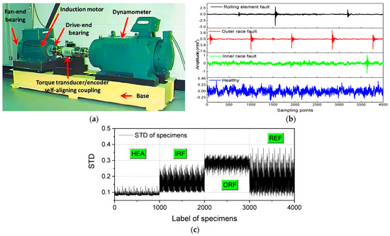
Figure 1.
(a) CWRU rolling bearing for fault simulation test bench in [17], (b) original signal of rolling bearing corresponding different states, (c) the standard deviation of all specimens.
Data acquisition was performed at a sampling frequency of 15 kHz, with the motor operating at a speed of 500, 700, and 900 rpm. Three distinct fault diameters of 0.21 mm, 0.33 mm, and 0.52 mm were simulated, representing inner race, outer race, and rolling element faults, respectively, along with a healthy condition. A sling window technique with a fixed sample length (4096) and a fixed sampling interval (2000) was employed to extract signal samples from the CWRU dataset.
Specifically, the vibration signals generated by the motor’s rolling bearings constitute a one-dimensional time series with temporal characteristics. The raw measurement signals corresponding to the four conditions, including healthy (HEA), inner race fault (IRF), outer race fault (ORF), and rolling element fault (REF) are illustrated in Figure 1b. The data used in the current database are collected under the same platform and conditions, so the samples in the dataset follow the same generation process or distribution. To evaluate its homogeneity and representativeness, the mean standard deviation is performed on the signals of 4000 samples (including four types of states), and the results are shown in Figure 1c.
Additionally, the original data are divided into datasets Φ1, Φ2, and Φ3 according to the three speeds. Then, for each given speed, 1000 samples were randomly selected and subsequently divided into training, testing, and verifying sets at a 7:2:1 ratio. This process then yielded a training set consisting of 2800 samples and a testing/verifying set containing 800/400 samples, both of which included all four defect categories (HEA, IRF, ORF, and REF), as tabulated in Table 1.

Table 1.
Details of the training and test corresponding to various speeds.
3. Signal Decomposition and Feature Extraction Model
3.1. Signal Reconstruction Method Based on ICEEMDAN and VMD
- Step I. Acquisition of high-frequency characteristics of signals
CEEMDAN (Complete Ensemble Empirical Mode Decomposition with Adaptive Noise) is a signal processing method designed to decompose complex signals into several Intrinsic Mode Functions (IMFs) [20]. While CEEMDAN reduces modal aliasing, it faces challenges in the early stages of decomposition due to the presence of significant noise and similar-scale features in the fault signals, which hinder the precise selection of IMFs. Kernel Principal Component Analysis (KPCA) can effectively extract non-linear features and reduce dimensionality by mapping data into a high-dimensional feature space, thereby efficiently handling complex datasets [21].
Therefore, incorporating KPCA into the CEEMDAN framework not only preserves the non-linear characteristics of the data but also eliminates redundant information, aiding in the extraction of more representative and discriminative non-linear principal components. This paper employs cross-analysis to determine the optimal component set, ensuring the retention of critical information during dimensionality reduction and the extraction of appropriate fractal dimensions of non-linear principal components. The flowchart of the improved CEEMDAN algorithm is presented in Figure 2.
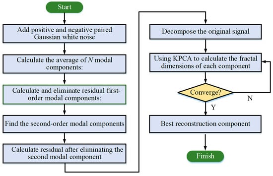
Figure 2.
Computation scheme of ICEEMDAN.
For bearing vibration signals, the first IMF component derived from the ICEEMDAN algorithm primarily encapsulates the high-frequency elements or the most dynamic portions of the original signal. Since high-frequency components are indicative of mechanical faults, the first IMF is crucial for early fault detection and diagnosis. The outcomes of signal decomposition for the four states using ICEEMDAN are illustrated in Figure 3 (one sample from each state listed in Table 1 was randomly chosen for demonstration, and IMFs are preset as 6).
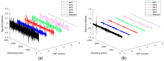
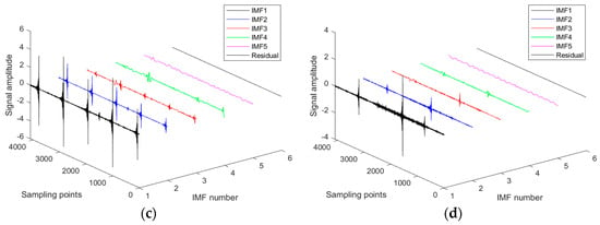
Figure 3.
Signal decomposition results via ICEEMDAN. (a) HEA, (b) IRF, (c) ORF, and (d) REF.
- Step II. Acquisition of high-frequency characteristics of signals
Since the first IMF from ICEEMDAN encompasses high-frequency components, VMD can further separate distinct characteristic frequencies within this high-frequency information [7], offering a more precise spectral analysis. This additional decomposition aids in clearly identifying these features, thereby improving the accuracy of fault detection. Additionally, the VMD algorithm effectively distinguishes between different frequency components, aiding in noise reduction and preserving more relevant signal features. The detailed V-IMF components derived from the VMD decomposition of IMF1, as illustrated in Figure 3, are shown in Figure 4 (the number of V-IMF components is preset as 7).
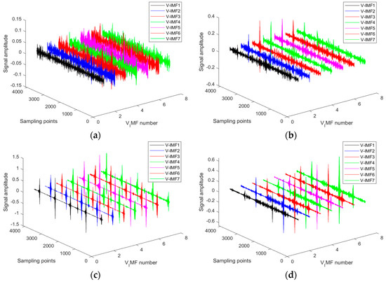
Figure 4.
Sub−signal decomposition results (V−IMF) via VMD. (a) HEA, (b) IRF, (c) ORF, and (d) REF.
3.2. Fault Feature Extraction Method Based on Improved Information Entropy (IIE)
Fault signals often introduce non-periodic or abrupt components into the signal. Information entropy highlights these anomalies, assesses the significance of various modes, and determines the purity of the signal, thereby assisting in fault diagnosis [22]. For the IMF components of vibration signals, a more ordered system corresponds to lower entropy values. The specific method for calculating information entropy is as follows.
For any variable X, the expression for information entropy H(X) is as follows:
In (1), pi is the ratio of the energy of the i-th IMF component to the total energy, and the IMF component is obtained from VMD (in Figure 4). The calculation formula for pi is as follows:
where x(t) is the input signal sequence concerning time t and Xi is the i-th signal.
When information entropy is used to describe bearing motion, fault-induced periodic impacts lead to a more ordered signal. Thus, IMF components containing fault signals will exhibit lower entropy values. However, during the early stages of bearing faults, the features may be less pronounced, resulting in lower identification rates. To address this, improvements to entropy are necessary, such as amplifying individual IMF features.
Additionally, kurtosis, an important indicator for describing waveform peaks and evaluating fault impacts, can enhance the model’s sensitivity to impact information. The entropy can be refined using kurtosis and is defined as follows:
In (3), Qi is the improved information entropy of the i-th IMF component and Hi and Ki are the information entropy and kurtosis indicators of the i-th IMF component, respectively. Since information entropy only represents the corresponding amount of IMF information, and due to environmental noise and other reasons, fault information does not show obvious entropy values.
Then, the number of IMFs decomposed from each specific signal segment is constant, and the improved information entropy of IMFs will have an upper limit value of the following:
In (4), n is the number of IMFs obtained by decomposition and Q is information entropy.
The average improved information entropy of a single set of original signals is as follows:
Compared to the unmodified entropy in (3) to (5), IIE uses kurtosis to improve the model’s sensitivity to impact information and address the issue of low recognition rates of entropy in less distinct fault components. Finally, relying on the above calculation process, the information entropy corresponding to the V-IMF obtained from VMD decomposition is calculated and used as the feature input (4000 × 7) for training CNN BiLSTM with different samples.
To examine the discrimination of these features in the case of state evaluation, t-distributed stochastic neighbor embedding (t-SNE) [23] is thus used for visualizing the formed feature input, and the resulting pictures are presented in Figure 5. The t-SNE algorithm, known for its efficiency and visualization capabilities in dimensionality reduction, aims to visualize the discrimination of features corresponding to different fault states. In Figure 5, 4000 signals with improved entropy (fault features, seven dimensions) are used as input, resulting in a three-dimensional fused feature representation (which lacks specific physical meaning). The visualization in Figure 5 shows that the signal features of different fault states (indicated by different colors) exhibit distinct regional distributions.
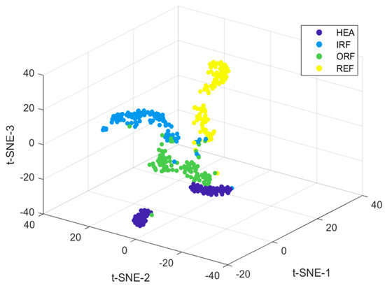
Figure 5.
The t-SNE results for visualizing the discrimination of feature input corresponding to various states.
4. Fault Diagnosis Model Based on Data-Driven and Deep Learning
4.1. MSCNN-BiLSTM-Based Fault Diagnosis Model Integrating an Attention Mechanism
In this study, spatial features are initially extracted using a feature selection layer and a multi-scale feature extraction layer, followed by temporal feature extraction through a BiLSTM layer. A self-attention mechanism is then introduced for adaptive fusion of all features, culminating in fault diagnosis results via a Softmax layer. The preliminary feature screening significantly impacts model performance. Bearing fault features are typically low-frequency signals; thus, larger convolution kernels are employed to enhance low-frequency feature extraction and suppress high-frequency noise, while also accommodating the periodic nature of vibration signals by providing a broader receptive field.
Consequently, the model utilizes large convolution kernels for initial feature screening, followed by batch normalization and max pooling layers to accelerate convergence and mitigate gradient issues. An optimized Inception module is employed to construct a multi-scale feature extraction module, thereby improving feature extraction capabilities at various scales. To further refine the network structure and enhance fault diagnosis accuracy, batch normalization is applied after each convolution operation to expedite training and prevent overfitting. Additionally, channel attention modules are integrated with post-post-feature extraction to generate and continuously optimize channel-specific weights. The self-attention mechanism effectively mitigates redundant feature interference and prevents loss of critical information, thus improving diagnostic performance. The mathematical expression for this process is as follows:
where Q, P, and V represent the query value, calculated value, and weight, respectively; f(Q, PT) is used to calculate the similarity between Q and P; dp is the feature vector dimension; and Softmax is a normalization function.
The feature extraction subnetwork and channel attention modules are alternately arranged to construct a multi-scale feature extraction module. This module continuously refines fault data by emphasizing critical features and suppressing noise, thereby enhancing diagnostic efficiency. Subsequently, features from different channels are merged and processed through a max pooling layer to retain essential characteristics and reduce model parameters. Spatial features extracted from the multi-scale feature extraction module are then fed directly into the BiLSTM layer to capture temporal information from vibration signals. Outputs from the BiLSTM layer are input to a self-attention mechanism to improve the network’s focus on global key features. Dimensionality reduction and information integration are performed via global average pooling, and the fault diagnosis results are ultimately produced by a Softmax classifier.
4.2. Computation Scheme and Parameter Values
Based on the previous sections, high-frequency signal components used to characterize fault features were obtained through ICCEMDAN and VMD decomposition. Subsequently, improved entropy was employed to achieve quantitative descriptions of different fault signals. Finally, a fault state evaluator was established using the entropy feature matrix based on the algorithm framework shown in Figure 6, with the entire algorithm framework illustrated in Figure 7.

Figure 6.
Multi-scale feature extraction module structure.
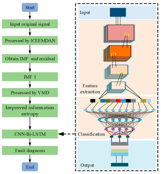
Figure 7.
Entire algorithm framework for fault diagnosis.
In the current work, the main hyper-parameter (HP) includes the number of IMFs in both ICEEMDAN and VMD, as well as the learning rate of MSCNN-BiLSTM. It can significantly affect the overall performance of algorithms; the selection of the optimal value of them is thus rather fundamental. Given the small parameter range and only three optimization variables in this case, iterative computation to determine optimal parameters is more suitable.
Therefore, we use ICEEMDAN and VMD to decompose all signals (4000 signals, the length of the signal is 4096), with the mean residuals serving as criteria for selecting the number of decompositions; accuracy on the validation set (400 signals) is used to choose the learning rate for MSCNN-BiLSTM. The criteria values corresponding to different parameters are shown in Figure 8. Under the condition of ensuring the highest accuracy of signal decomposition and the evaluation results, the number of IMFs in ICEEMDAN and VMD is five and seven, respectively, and the learning rate for MSCNN-BiLSTM is 0.006.

Figure 8.
The criteria values correspond to different parameters: (a,b) are the number of IMFs, (c) is the learning rate.
Given that model parameters significantly impact signal processing results and the final evaluation outcomes, the parameters listed in Table 2 were used throughout all sample data preprocessing, feature extraction, and training. Finally, Figure 9 presents the accuracy (using a test set in Table 1) during the 50 iterations, in which the computation is completed by a computer with a 2nd Gen Intel(R) Core(TM) i9-12900K CPU at 3.20 GHz and a 64 bit Win 11 system with 16.0 GB of RAM. The Matlab Deep Learning Toolbox is used in this work for fault diagnosis. The computation time is 144 s. Obviously, the final accuracy of the test set is close to 98%.

Table 2.
Parameter values used in the contained models.
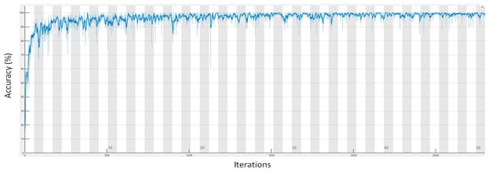
Figure 9.
The diagnosis accuracy during the iterations.
5. Verification for Fault Diagnosis
5.1. Diagnosis Results Analysis
The training and testing sets with sample sizes of 2800 and 800, respectively, are used to train the fault assessment for motor bearings in four different states. The internal parameters and training process of the evaluator are detailed in Table 2 and Figure 9. Additionally, a validation set with a sample size of 400 (details in Table 3) is used to assess the accuracy of the constructed evaluator. First, the ICCEMDAN decomposition is applied to the 400 validation vibration signals based on the computation process shown in Figure 8. Then, the first IMF component obtained is further decomposed using VMD to obtain 7 V-IMF components. Next, the improved entropy of each V-IMF is calculated and used as feature inputs for the fault evaluator. Finally, the evaluation state is obtained through the CNN-BiLSTM model with an attention mechanism. Figure 10a shows the final confusion matrix, and Figure 10b compares the evaluations and actual states for different fault conditions. It can be seen that the reported evaluator achieves an overall assessment accuracy of 99.25%, with fault assessment accuracy reaching 100% for HEA and ORF states.

Table 3.
Details of the used verification set.
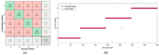
Figure 10.
(a) Confusion matrix of the evaluation results. (b) Comparison of the evaluated and actual states.
5.2. Comparison of Fault Diagnosis Accuracy via Different Models
To demonstrate that the current model combining multiple processing methods is optimal, this section conducts comparative experiments using the same sample data. Specifically, the models ICEEMEDAN-VMD-IIE-CNN, VMD-IIE-CNN-BiLSTM, and ICEEMDAN-IIE-CNN-BiLSTM are selected. The algorithm parameters and computational conditions are consistent with those described in Section 5.1.
Then, Figure 11 presents the confusion matrices for the three combined models mentioned above. Table 4 shows the fault state assessment accuracy for each model. The differences in classifiers have a minimal impact on overall accuracy, while the reconstruction (decomposition) methods for signals are crucial for the assessment. In summary, it is evident that the method reported in this paper effectively extracts fault features from samples, ensuring high accuracy in state evaluation.
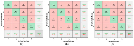
Figure 11.
Accuracy of the evaluation results. (a) ICEEMEDAN-VMD-IIE-CNN, (b) VMD-IIE-CNN-BiLSTM, (c) ICEEMDAN-IIE-CNN-BiLSTM.

Table 4.
Accuracy comparison of the evaluation results of various combinations.
Table 4 compares the proposed ICEEMEDAN-VMD-IIE-CNN with VMD-IIE-CNN-BiLSTM and ICEEMDAN-IIE-CNN-BiLSTM to highlight the contribution of ICEEMEDAN-VMD. According to this comment, we added the additional methods (SVM, GRNN, and DPRNN), and a detailed table of comparison with the state-of-the-art methods is tabulated in Table 5.

Table 5.
Accuracy comparison of the evaluation results corresponding to various models.
In the experiments, “×” indicates non-applicability, with decomposed signals used as feature inputs. The SVM parameters are set with a penalty factor of 0.1 and a radial basis function kernel; the GRNN parameters include a spread parameter of 0.5. The DPRNN parameters are configured as follows: seven layers, a stride of 1, ReLU activation function, a dropout rate of 0.3, a learning rate of 0.001, a batch size of 64, and the Adam optimizer. All other computational and sample conditions remain consistent.
According to the results, the impact of different classifiers on the evaluation outcomes is not significant when the signal reconstruction and feature extraction methods are the same. This is because the input features already exhibit good separability, as demonstrated by the TSNE results in Figure 5 in the revised manuscript.
6. Conclusions
Given the faced shortcomings, this work proposed an intelligent strategy for fault diagnosis via the combination of signal reconstruction and deep learning, and the current findings lead to the following conclusions.
The strategy of combining ICEEMDAN and VMD enables adaptive signal decomposition, streamlining fault feature extraction through improved information entropy and avoiding the complexities of manual feature extraction while significantly enhancing computational efficiency. The developed fault classifier not only captures multi-scale spatial and temporal features but also integrates a channel attention mechanism, which improves the model’s ability to select and extract fault features.
The comparative experimental results demonstrate that the proposed model exhibits strong generalization and versatility, maintaining high fault diagnosis accuracy (99.25%) under varying speeds and noisy conditions, outperforming comparison models. However, due to the low number of training and test samples, as well as the optimization of hyper-parameters and algorithm architecture, further testing and research are needed to assess its applicability to other bearing faults and mixed fault scenarios.
Author Contributions
Conceptualization, W.L. and N.F.; methodology, C.Z.; software, C.Z. and M.L.; validation, X.Y.; formal analysis, L.M.; investigation, W.L. and X.P.; resources, N.F.; data curation, W.L. and N.F.; writing—original draft preparation, L.M.; writing—review and editing, M.L. and N.F.; project administration, W.L. All authors have read and agreed to the published version of the manuscript.
Funding
This research received no external funding.
Data Availability Statement
The data supporting the findings of this study are available from the corresponding author upon reasonable request due to the difficulty in obtaining experimental data.
Conflicts of Interest
The authors declare no conflicts of interest.
References
- Hu, Z.X.; Wang, Y.; Ge, M.F.; Liu, J. Data-Driven Fault Diagnosis Method Based on Compressed Sensing and Improved Multi-Scale Network. IEEE Trans. Ind. Electron. 2020, 67, 3216–3225. [Google Scholar] [CrossRef]
- Shao, H.D.; Xia, M.; Han, G.J.; Zhang, Y.; Wan, J. Intelligent Fault Diagnosis of Rotor-Bearing System under Varying Working Conditions with Modified Transfer CNN and Thermal Images. IEEE Trans. Ind. Inform. 2021, 17, 3488–3496. [Google Scholar] [CrossRef]
- Knap, P.; Lalik, K.; Balazy, P. Boosted Convolutional Neural Network Algorithm for the Classification of the Bearing Fault from 1-D Raw Sensor Data. Sensors 2023, 23, 4295. [Google Scholar] [CrossRef]
- Gao, L.; Li, X.K.; Yao, Y.C.; Wang, Y.; Yang, X.; Zhao, X.; Geng, D.; Li, Y.; Liu, L. A Modal Frequency Estimation Method of Non-Stationary Signal under Mass Time-Varying Condition Based on EMD Algorithm. Appl. Sci. 2022, 12, 8187. [Google Scholar] [CrossRef]
- Guo, M.F.; Zeng, X.D.; Chen, D.Y.; Yang, N.C. Deep-Learning-Based Earth Fault Detection Using Continuous Wavelet Transform and Convolutional Neural Network in Resonant Grounding Distribution Systems. IEEE Sens. J. 2017, 18, 1291–1300. [Google Scholar] [CrossRef]
- Zhang, Z.; Deng, A.; Wang, Z.; Li, J.; Zhao, H.; Yang, X. Wind Power Prediction Based on EMD-KPCA-BiLSTM-ATT Model. Energies 2024, 17, 2568. [Google Scholar] [CrossRef]
- Wang, D.; Li, S.; Fu, X. Short-Term Power Load Forecasting Based on Secondary Cleaning and CNN-BILSTM-Attention. Energies 2024, 17, 4142. [Google Scholar] [CrossRef]
- Zhang, Z.; Liu, X.; Zhang, X.; Yang, Z.; Yao, J. Carbon Price Forecasting Using Optimized Sliding Window Empirical Wavelet Transform and Gated Recurrent Unit Network to Mitigate Data Leakage. Energies 2024, 17, 4358. [Google Scholar] [CrossRef]
- Huang, N.E.; Shen, Z.; Long, S.R.; Wu, M.C.; Shih, H.H.; Zheng, Q.; Yen, N.-C.; Tung, C.C.; Liu, H.H. The Empirical Mode Decomposition and the Hilbert Spectrum for Nonlinear and Non-Stationary Time Series Analysis. Proc. Math. Phys. Eng. Sci. 1998, 903, 903–995. [Google Scholar] [CrossRef]
- Wu, Z.; Huang, N.E. Ensemble Empirical Mode Decomposition: A Noise Assisted Data Analysis Method. Adv. Adapt. Data Anal. 2009, 1, 1–41. [Google Scholar] [CrossRef]
- Konstantin, D.; Dominique, Z. Variational Mode Decomposition. IEEE Trans. Signal Process. 2013, 62, 531–544. [Google Scholar]
- Li, Z.; Chen, J.; Zi, Y.; Pan, J. Independence-Oriented VMD to Identify Fault Feature for Wheel Set Bearing Fault Diagnosis of High-Speed Locomotive. Mech. Syst. Signal Process. 2017, 85, 512–529. [Google Scholar] [CrossRef]
- Ding, L.; Guo, H.; Bian, L. Convolutional Neural Networks Based on Resonance Demodulation of Vibration Signal for Rolling Bearing Fault Diagnosis in Permanent Magnet Synchronous Motors. Energies 2024, 17, 4334. [Google Scholar] [CrossRef]
- Tama, B.A.; Vania, M.; Lee, S.; Lim, S. Recent advances in the application of deep learning for fault diagnosis of rotating machinery using vibration signals. Artif. Intell. Rev. 2023, 56, 4667–4709. [Google Scholar] [CrossRef]
- Chen, X.H.; Yang, R.; Xue, Y.H.; Huang, M.; Ferrero, R.; Wang, Z. Deep Transfer Learning for Bearing Fault Diagnosis: A Systematic Review Since 2016. IEEE Trans. Instrum. Meas. 2023, 72, 3508221. [Google Scholar] [CrossRef]
- Qiao, M.Y.; Yan, S.H.; Tang, X.X.; Xu, C. Deep Convolutional and LSTM Recurrent Neural Networks for Rolling Bearing Fault Diagnosis under Strong Noises and Variable Loads. IEEE Access 2020, 8, 66257–66269. [Google Scholar] [CrossRef]
- Hao, S.J.; Ge, F.X.; Li, Y.M.; Jiang, J. Multisensor Bearing Fault Diagnosis Based on One-Dimensional Convolutional Long Short-Term Memory Networks. Measurement 2020, 159, 107802. [Google Scholar] [CrossRef]
- Guo, Y.R.; Mao, J.; Zhao, M. Rolling Bearing Fault Diagnosis Method Based on Attention CNN and BiLSTM Network. Neural Process. Lett. 2023, 55, 3377–3410. [Google Scholar] [CrossRef]
- Case Western Reserve University Bearing Data Center Website. 2013. Available online: https://engineering.case.edu/bearingdatacenter/ (accessed on 31 January 2023).
- Li, Z.W.; Xu, H.Y.; Jiang, B.B.; Han, F. Wavelet Threshold Ultrasound Echo Signal Denoising Algorithm Based on CEEMDAN. Electronics 2023, 12, 3026. [Google Scholar] [CrossRef]
- Pan, H.; Badawi, D.; Bassi, I.; Ozev, S.; Cetin, A.E. Detecting Anomaly in Chemical Sensors via L1-Kernel-Based Principal Component Analysis. IEEE Sens. Lett. 2022, 6, 7004304. [Google Scholar] [CrossRef]
- Zivieri, R. Magnetic Skyrmions as Information Entropy Carriers. IEEE Trans. Magn. 2022, 58, 1500105. [Google Scholar] [CrossRef]
- Fu, Y.; Zhou, K.; Zhu, G.; Li, Z.; Li, Y.; Meng, P.; Xu, Y.; Lu, L. A Partial Discharge Signal Separation Method Applicable for Various Sensors Based on Time–Frequency Feature Extraction of t-SNE. IEEE Trans. Instrum. Meas. 2024, 73, 3505609. [Google Scholar] [CrossRef]
Disclaimer/Publisher’s Note: The statements, opinions and data contained in all publications are solely those of the individual author(s) and contributor(s) and not of MDPI and/or the editor(s). MDPI and/or the editor(s) disclaim responsibility for any injury to people or property resulting from any ideas, methods, instructions or products referred to in the content. |
© 2024 by the authors. Licensee MDPI, Basel, Switzerland. This article is an open access article distributed under the terms and conditions of the Creative Commons Attribution (CC BY) license (https://creativecommons.org/licenses/by/4.0/).