Methods for the Investigation and Mitigation of Conducted Differential-Mode Electromagnetic Interference in Commercial Electrical Vehicles

Abstract

One of the main challenges as the market for fully commercial electrified vehicles quickly expands is predicting the electromagnetic interference (EMI) in traction voltage systems (TVSs) in differential mode (DM) and common mode (CM). The number of subsystems connected to vehicle TVSs is increasing, and thus, so are the electromagnetic compatibility (EMC) requirements. These requirements should make sure that neither the function nor lifetime of any source or load is affected by another, but experience shows that they are often insufficient. The purpose of this article is to show how circuit simulations can complement these requirements and that a generalized artificial network/line impedance stabilization network (LISN) is insufficient to correctly predict the EMI situation of a real vehicle. This article presents a method for complexity reduction in TVS DM simulations and a comparison with the usage of LISN to predict the EMI between subsystems; the article also addresses how to mitigate the EMI with DM filters for the subsystems. The proposed method creates a foundation for a faster and safer development process. The simulation model’s development includes a traction battery and TVS subsystems. It is found that a standardized LISN does not reflect the behavior of a commercial TVS and cannot be used solely to judge if a subsystem will operate as intended within a TVS without creating EMI. A change in switching frequency in the DUT can cause severe resonance between TVS subsystems, but this is not seen with a LISN. The conclusion of the article is that LISN can provide a false sense of security and that calibrated simulation models of a complete TVS are necessary to predict the behavior in that TVS; this study also highlights the importance of using DM filters to ensure protection against resonance frequencies.

1. Introduction

The market for commercial electrified vehicles is quickly expanding. This also increases the need for early validation of the electric behavior of traction voltage systems (TVSs) and the included subsystems.

The TVS of a road vehicle, such as a heavy-duty truck or a car, is a class B voltage (<1500 V DC) system, and such systems include traction battery packs (BPs) and all subsystems that are connected to the traction batteries, including electric machine drives (EMDs), air compressor drives, and DC/DC converters. All subsystems use power electronic switches and, thus, are sources of high-bandwidth excitation of the very complex impedance network that makes up the TVS with all of its subsystems. It is a challenge to ensure a sustainable electromagnetic interference (EMI) situation given the multitude of configurations of TVSs in different versions and models of vehicles. Ref. [1] presents a method for analyzing and quantifying the interference in high-voltage DC (HV-DC) systems due to excitation currents from inverters based on impedance, frequencies, and operating points. Avoiding damage or aging due to current ripple is crucial when it comes to expensive parts in a fuel cell electric heavy-duty truck (FCEHDT) and is discussed in [2]. There are quite a few publications that focus on a single subsystem, such as the single-motor drive and its formation of harmonics on its DC side [3,4,5,6,7] and the DC-link capacitor [8] and how these age DC capacitors [9]. However, there are not many publications that describe the challenges of modeling and simulating entire systems such as the traction systems in trucks. It is important to be able to predict the EMI situation in new TVS configurations or when new subsystems, e.g., from a new supplier, are introduced. This requires simulation models. The purpose of simulation models is to gain confidence in the design phase that the connected TVS subsystems will work together at a sustainable level of EMI and to predict what electromagnetic interference (EMI), in terms of currents and voltages, can be expected in the vehicle at the prototype and production stages. Unexpected EMI in a prototype vehicle will delay its market introduction and decrease possibilities for changing unwanted behaviors in subsystems.

The simulation models must represent the high-frequency voltage and current content that are associated with both differential-mode (DM) and common-mode (CM) electromagnetic disturbances [10,11], which can reach up to at least 10 MHz for the CM and 100 kHz for the DM. However, simulation models of complete TVSs, including feedback loops in subsystems, become large due to the high-frequency content, meaning that they are slow to simulate and not practically usable. Simplifications that capture relevant phenomena with minimum complexity are needed. A standardized form of a simplified simulation model is an artificial network referred to as the line impedance stabilization network (LISN). It is supposed to mimic the impedance characteristics of electric networks in the connection point of a subsystem.

This study achieves the following:

• It describes how the modeling and simulation of a TVS can be simplified to a practically functional level that assists in setting requirements for subsystems that make sure that neither the function nor lifetime of any source or load is severely affected by another.
• It describes how to verify subsystems from suppliers created for original equipment manufacturers (OEMs).
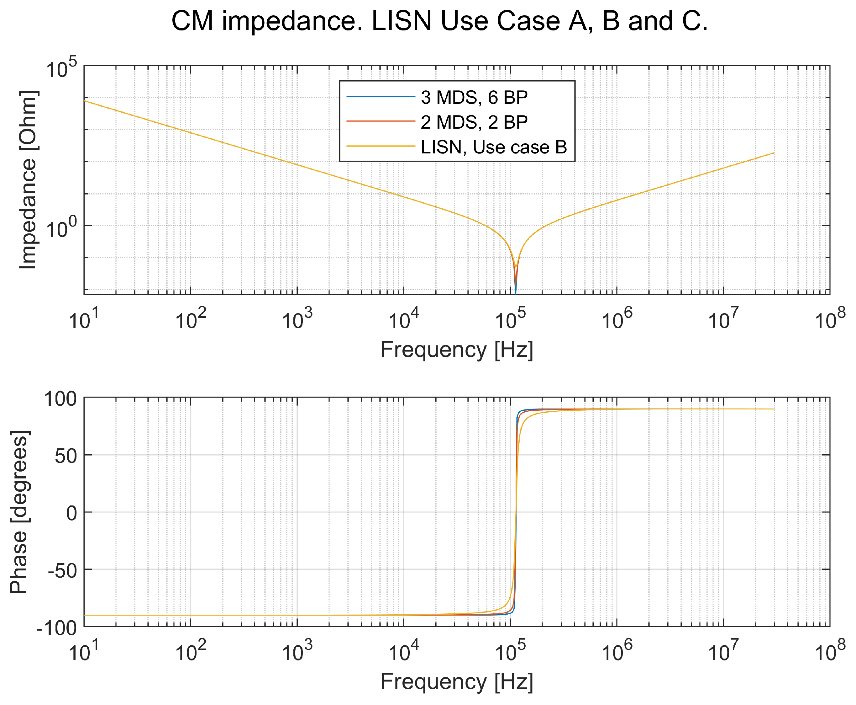
• It presents a comparison of simulations of the traction voltage system (TVS) in a commercial electric vehicle, with several levels of simplifications, and an LISN. A recommendation from this article is that the customer should use a tailored LISN [12] that reflects their specific vehicle(s); in real vehicles, impedance differs too much from the impedance of a standardized artificial network [13,14]. It is also recommended to perform simulations to foresee behavior within TVSs that is not reflected at all by the LISN.
• This study also shows the importance of DM filters in subsystems to avoid resonances in a TVS. If a resonance frequency is triggered by a switching device, it may cause high-ripple currents that may accelerate the aging of the DC-link capacitor. In electric traction machine drives, the worst operating point with respect to the current that flows in the DC-link capacitor is at about half the base speed combined with the maximum torque [15].

N.B.: The simulations presented in this article are partly verified using a vehicle with a TVS that includes three machine drive systems (MDSs) and several auxiliaries. One MDS consists of one EMD and one electric machine (EM). It is difficult to find the same operating point in a simulation as in a measurement, because real loads operate as stand-alone systems, and switching events are not synchronized. The simulation model and details of the traction voltage system are not shared due to intellectual property (IP) concerns.

The rest of this article is structured in the following way.

In Section 2, a comprehensive model of all relevant subsystems and their aggregates in a TVS, representing both DM and CM properties and the effect of feedback loops, is introduced. Furthermore, it is shown how the subsystem models can be simplified without losing relevance with respect to DM and CM EMI. Comparisons with detailed in-truck measurements are made. A comparison with the use of a standardized LISN is made, and suggestions on how to alter an LISN to increase its relevance compared with the complete circuit simulation are provided. Finally, a circuit simulation is used to show the importance of introducing a DM filter on the DC terminals of subsystems in a TVS.

In Section 3, the developed simulation models from Section 2 are used to emphasize the difference between details in the DC DM current drawn by an EMD using a full-circuit simulation compared with using an LISN. It is also shown how an LISN fails to reveal how a change in the configuration and number of batteries and traction machines may lead to very significant differences in the frequency content of the DC-link current drawn by a specific subsystem. Finally, the impact of a DM filter on the DC terminals of subsystems in the TVS is quantified.

In Section 4, the results from the model development and simplifications are discussed, and in Section 5, the main conclusions and recommendations for future work are discussed.

2. Modeling, Verification, and Simulations

This section is dedicated to TVS modeling and model calibration. The subject for the measurements and simulations is a commercial truck’s traction voltage system (TVS), as shown in Figure 1.

The main functions of the TVS shown in Figure 1 are described in

Table 1. The main functions of the TVS shown in Figure 1.

Subsystem	Description
EMD1–EMD3	The electrical machine drive (EMD) provides electrical energy to or from the electrical machine (EM). The EMD converts DC to AC and AC to DC.
EM1–EM3	The electrical machines (EMs) convert electrical energy into mechanical energy to propel the vehicle or convert mechanical energy into electrical energy to brake the vehicle.
Gearbox	This changes the speed from the EM to the shaft. The use of a gearbox makes the use of EMs more efficient, as the speed of the EMs can be higher; thus, the EMs are smaller in volume and cheaper in cost.
BP1–BP6	A battery pack (BP) stores energy that is charged from the grid. It also provides the vehicle with energy for consumers and receives energy from the EMD when braking the vehicle.
OCEPS	The onboard charger and electrical power supply (OCEPS) charge the batteries when connected to the AC grid.
CSU	The charging switch unit (CSU) is mainly a contactor that is isolated when not charging.
DCDC1–DCDC2	The DC/DC is a converter that supplies the 24 V batteries with energy from the BP.
El. Heater Cab	The electrical cab heater is a heater that provides heat to the driver’s cab.
El. Heater Bat	The electrical battery heater is a heater that provides heat to the batteries.
AC Compr	The air-conditioning compressor provides cooling to the driver’s cab.
Air Compr	The air compressor provides compressed air to the vehicle, mainly for the brakes.
JB, JB1–JB3	The junction boxes (JBs) provide connections between the different components of the TVS. The high-current consumers, such as the EMD and BPs, connect via busbars, and the low-current consumers are connected via fuses.
Orange cables	The “orange cables” are coaxial or twin axial cables that provide shielding and a return path for common-mode currents.

.

The purpose of the measurements and simulations is to verify that the subsystems included in the TVS do not disturb each other with conducted electromagnetic interference (EMI). Conducted EMI may lead to functional disturbances or a decreased lifetime of the components. This article focuses on differential-mode (DM) disturbances. Common-mode (CM) disturbances and how to mitigate them are described in [15,16,17,18].

2.1. Measurements for Model Calibration

Simulation models are designed to match measurements of subsystems [16]. Some subsystems are available for “tear-down”, and some are just measured from the outside, e.g., at the positive and negative poles.

To obtain measurements of the impedance to create a simulation model of a subsystem, it is convenient to use an LCR meter (L—inductance; C—capacitance; R—resistance). This is an instrument made to analyze the frequency characteristics of various types of subsystems. The LCR meter used in the work presented in this article was a PSM3750 Frequency Response Analyzer [19] with an IAI2 Impedance Analyzer [20], as shown in Figure 2.

One common method of measuring impedance is the four-wire Kelvin method with Kelvin leads, as shown in Figure 3 and Figure 4. During testing, it was found that the method was not accurate above 4–5 MHz, as the Kelvin leads introduced capacitance and inductance in the circuit.

Measurements on a battery or DC source were not possible with this LCR instrument because the device under test (DUT), in this case, had an internal DC voltage source that was far too high. The normal procedure is to measure passive circuits as resistors, capacitors, inductors, or a mix thereof. If measurements shall be made on devices with an internal DC voltage, the DC voltage needs to be blocked. There are no high-voltage (HV) LCR interfaces for voltages around 750 V DC available on the market, or at least they were not found by the author of this article. Instead, an HV LCR interface was developed, and a principal schematic thereof is shown in Figure 5. In Figure 5, “Gen” is the generated output signal from the LCR meter, “Ch2” measures the current of the “Gen” signal, and “Ch1” measures the voltage at the DUT.

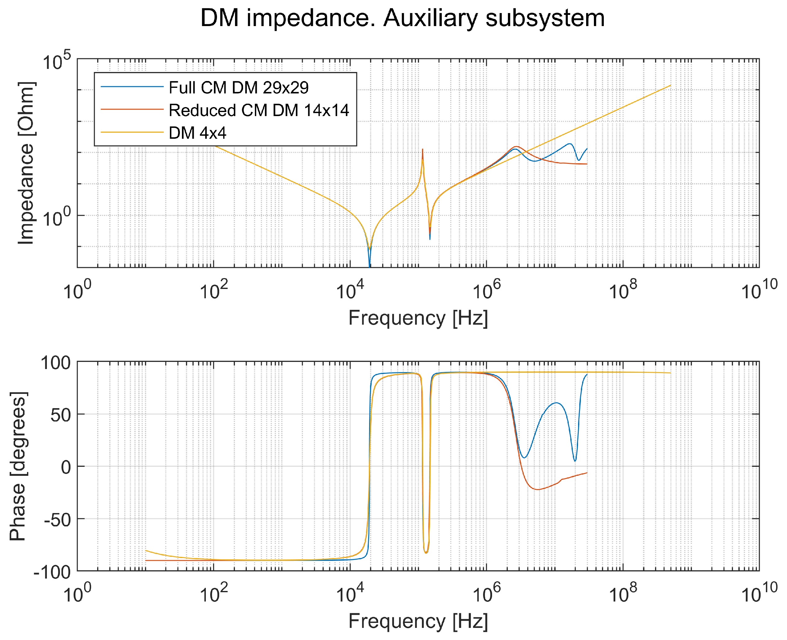
2.2. Simplification of System Simulation in PLECS

Simulations were performed in the PLECS simulation platform [21], version 4.8.8 (64 bit). The measured data from Section 2.1 were used to build subsystem models in PLECS. The DM impedance characteristics of all subsystems of a complete TVS in Figure 1 were modeled and found to be valid up to 100 kHz. In this study, simulations of the DM were performed, and it was found that the fully detailed combined CM and DM models could not be used for DM simulations because the models were too large, complex, and stiff. A model that is too stiff appears when there is a system of differential equations in which certain components interact in a very short time and remain constant while others change slowly. Stiff models often appear in simulations of electrical circuits, especially when considering parasitic parameters such as inductance and capacitance. The subsystems that are modeled have all of these constraints. A way forward is to reduce the models to smaller state–space matrices without losing data in the required frequency range of interest. The full system, representing both CM and DM parameters, grew to exceed a 500 × 500 state–space matrix.

The size of a state–space matrix is, in practice, impossible to simulate, even with the fastest desktop computers. The reason for this is that many parasitic elements with small values, representing very short time constants, and a high number of switching elements (power electronics), which also require a high time resolution, make the state–space matrix “very stiff”. This can be solved by means of two different approaches.

(I)

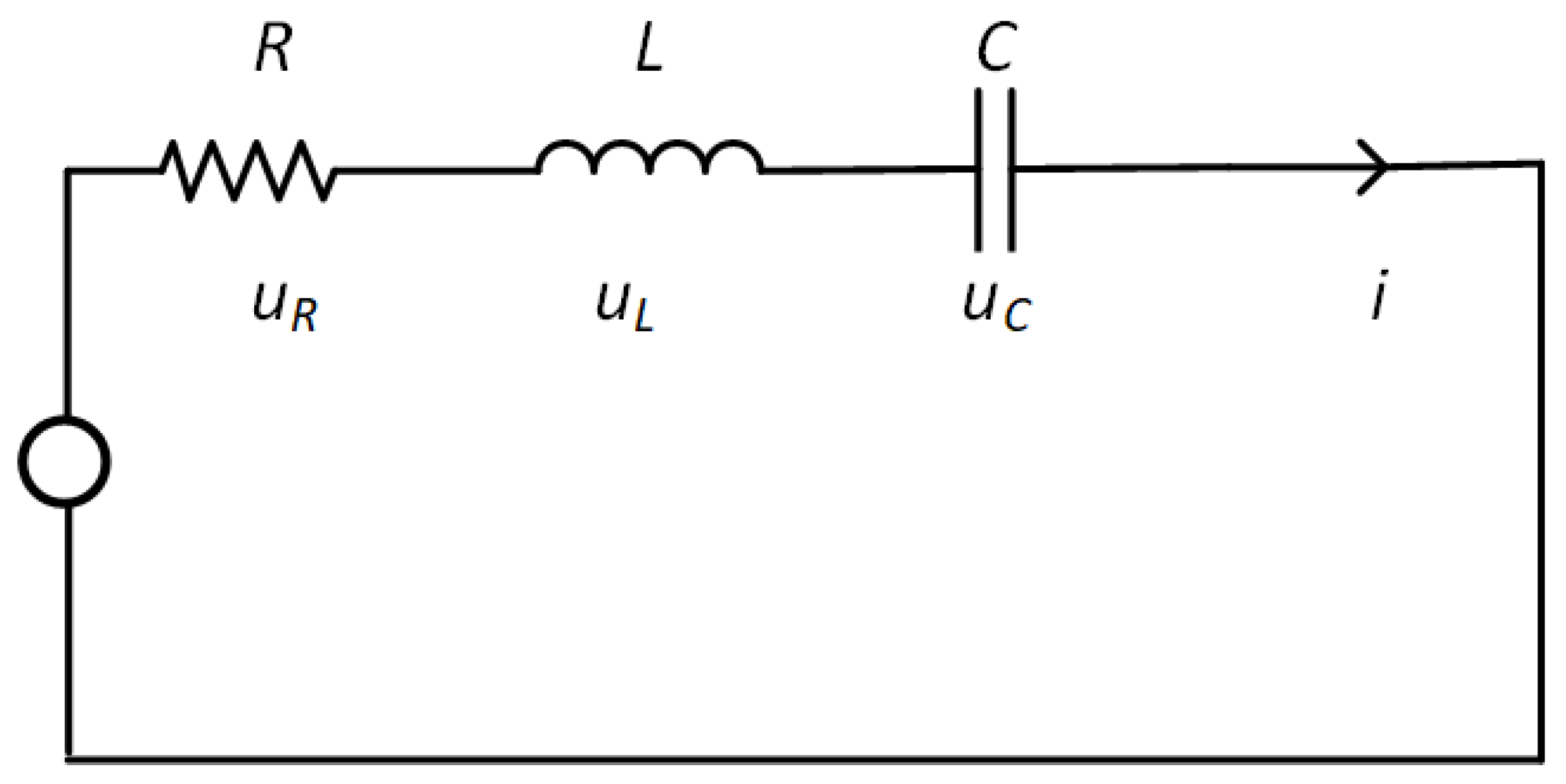
The first is the elimination of parasitic and/or intentional circuit parameters that have no or negligible impact on the simulation results in the frequency range of interest. There is, to the knowledge of the authors, no straightforward way to find candidates for parameters to eliminate, but a “qualified cut and try” approach has been successfully implemented. A model that represents a discrete component, subsystem, or vehicle system can be represented by a state–space matrix. In the simulation tool, the matrices are not the primary interface to work with, but they are useful for determining the eigenvalues of the circuit. To understand the method, a simple model is presented in Figure 6.

The state–space matrix is written as follows:

$$\dot{x}=Ax+Bu$$

(1)

$$y=Cx+Du$$

(2)

From Figure 6, the A-matrix is obtained as follows:

$$\begin{array}{c}A=\left[\begin{array}{cc}-{\displaystyle \frac{R}{L}}& -{\displaystyle \frac{1}{L}}\\ {\displaystyle \frac{1}{C}}& 0\end{array}\right]\end{array}$$

(3)

The natural resonance frequency is described in Equation (4).

$${\omega }_n={\displaystyle \frac{1}{\sqrt{LC}}}$$

(4)

In TVSs, many combinations of L and C form all of the natural frequencies, but a “qualified cut and try” approach has been successfully implemented. For example, combinations of small values of L and C that result in natural frequencies higher than those of interest can be found.

(II)

The second approach is the replacement of switching elements with ramped current sources. This method is described in detail in Section 2.3.

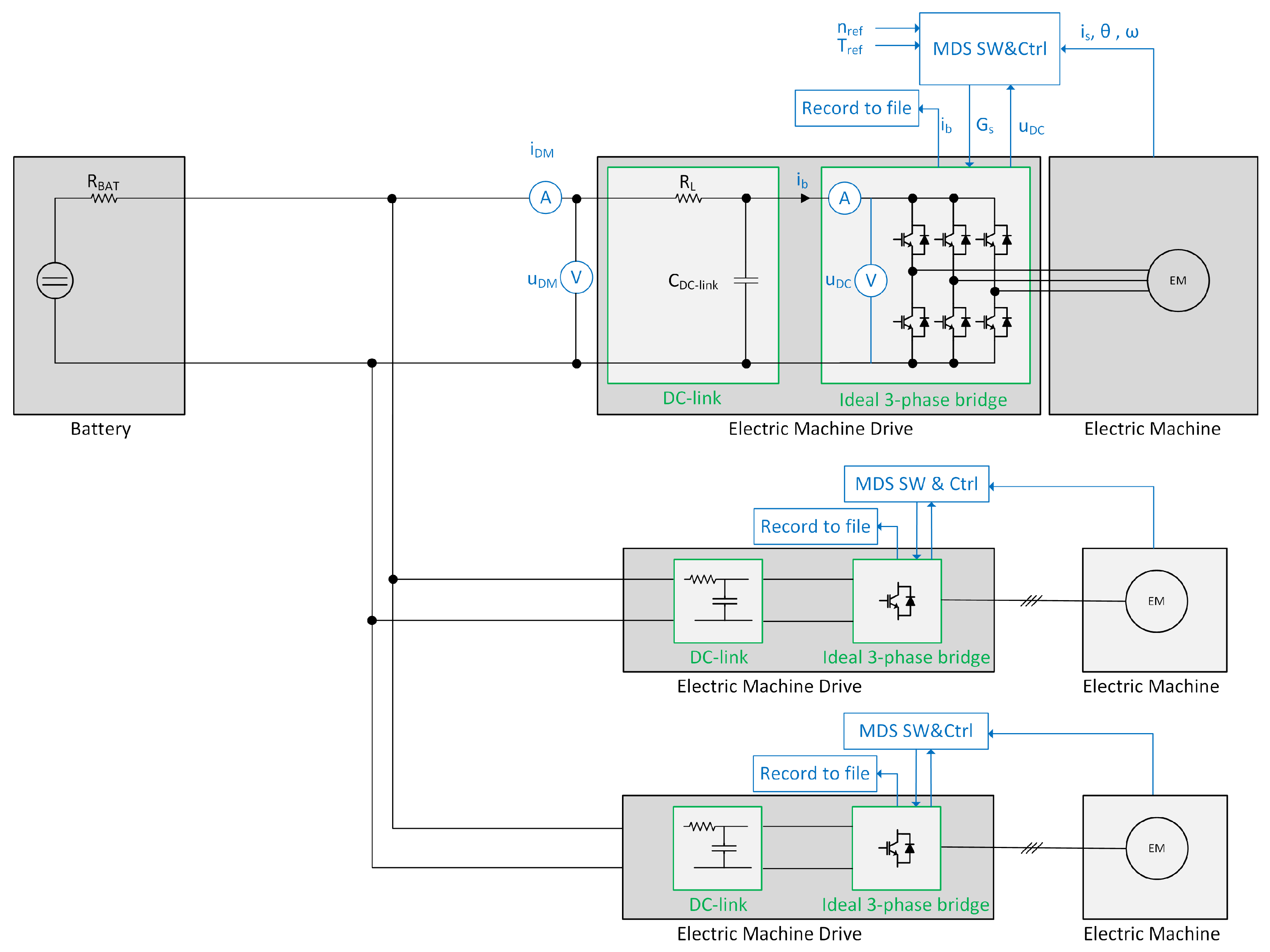
2.3. Subsystem Simplification for DM Simulation in PLECS

A reduction of a subsystem, according to the approach in Section 2.2, is a subsystem with DM and CM parameters, such as the series resistance of inductors, inductance of cables, or capacitance from the TVS to the chassis, that gives a complete state-space matrix of 29 × 29. To model the CM aspects only, it can be reduced to 14 × 14 while keeping the impedance in the required frequencies. To account for the DM aspect only, it can be reduced to 4 × 4. In Figure 7, the three models are compared from a DM perspective.

The evaluation of the DM impedance for the auxiliary system in Figure 7 is made up to a maximum of 100 kHz, and it is shown that the reduced model is accurate even up to 1 MHz. The limit of 100 kHz is due to the measurements in a vehicle that show that higher RMS values of DM currents in the TVS measured in the truck are negligible according to Figure 1, such as $i_{DM\_EMD1}$ and $i_{DM\_DCDC1}$.

All included subsystems are integrated to form a simulation model of the full TVS, as shown in Figure 1.

2.4. System Simulation Model in PLECS for DM

From this point, all of the models of the subsystems are available, and full simulations are performed.

There is a challenge when modeling power–electronic converters, such as the 3-phase converter in an EMD. In system simulations, the switches and the DC-link capacitor are most easily modeled as ideal. With ideal capacitor models, the DC DM currents’ appearance in simulations differs from measurements. A capacitor’s stray inductance within a DC-link capacitor is needed to determine the correct appearance of the DC DM current $i_{DM}$, as shown in Figure 8. Using ideal switches in a three-phase converter gives an infinite transient voltage over the DC link. Modeling insulated-gate bipolar transistors (IGBTs) in PLECS with limited rise and fall time causes the model to stiffen. To handle this challenge, an ideal simulation is performed, and the current $i_b$ to the three-phase bridge is recorded, as shown in Figure 8.

To handle the unwanted effects of ideal switch models and to speed up system simulations, the following steps are taken.

• A reduced system model with a complete MDS with active feedback control is simulated with an ideal battery and ideal cables; see Section 2.4.1.
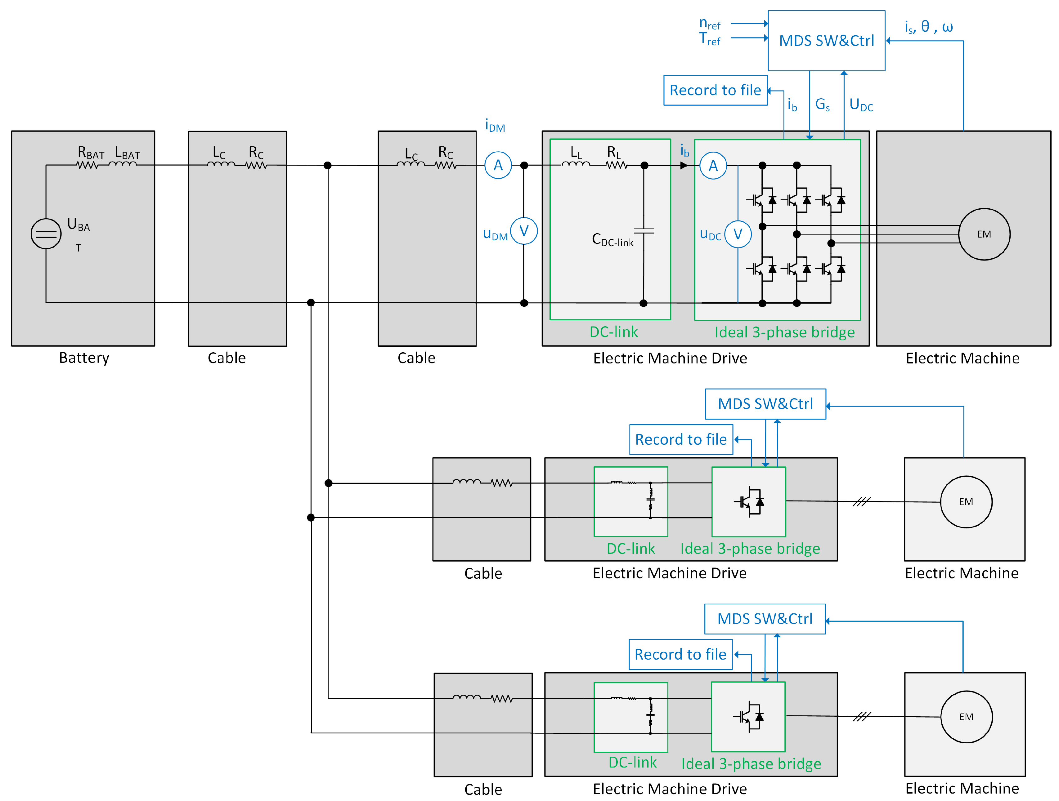
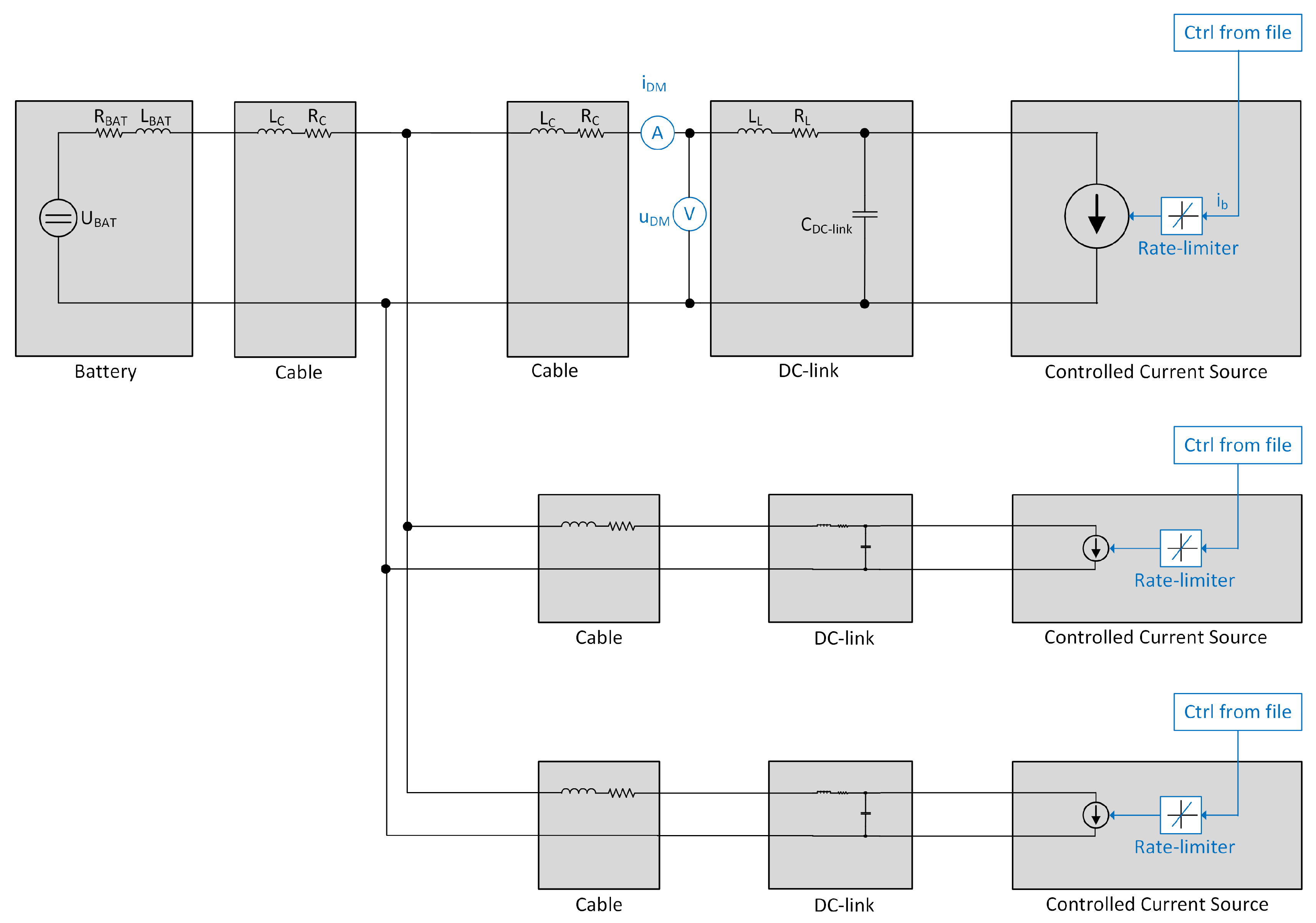
• An extended system model with DC cable models and refined battery and EMD models is simulated. The full EMD of step 1 is replaced with a DC current source mimicking the DC-link current drawn by the MDS of step 1, and a slew rate is added to the DC-link current pulses. This model thus uses a more advanced system model but with an EMD behavior as an ideal model; see Section 2.4.2.
• An extended system model with a complete MDS with active feedback control is simulated; see Section 2.4.3. It is the same case as in item 2 but with the complete MDS, including feedback.
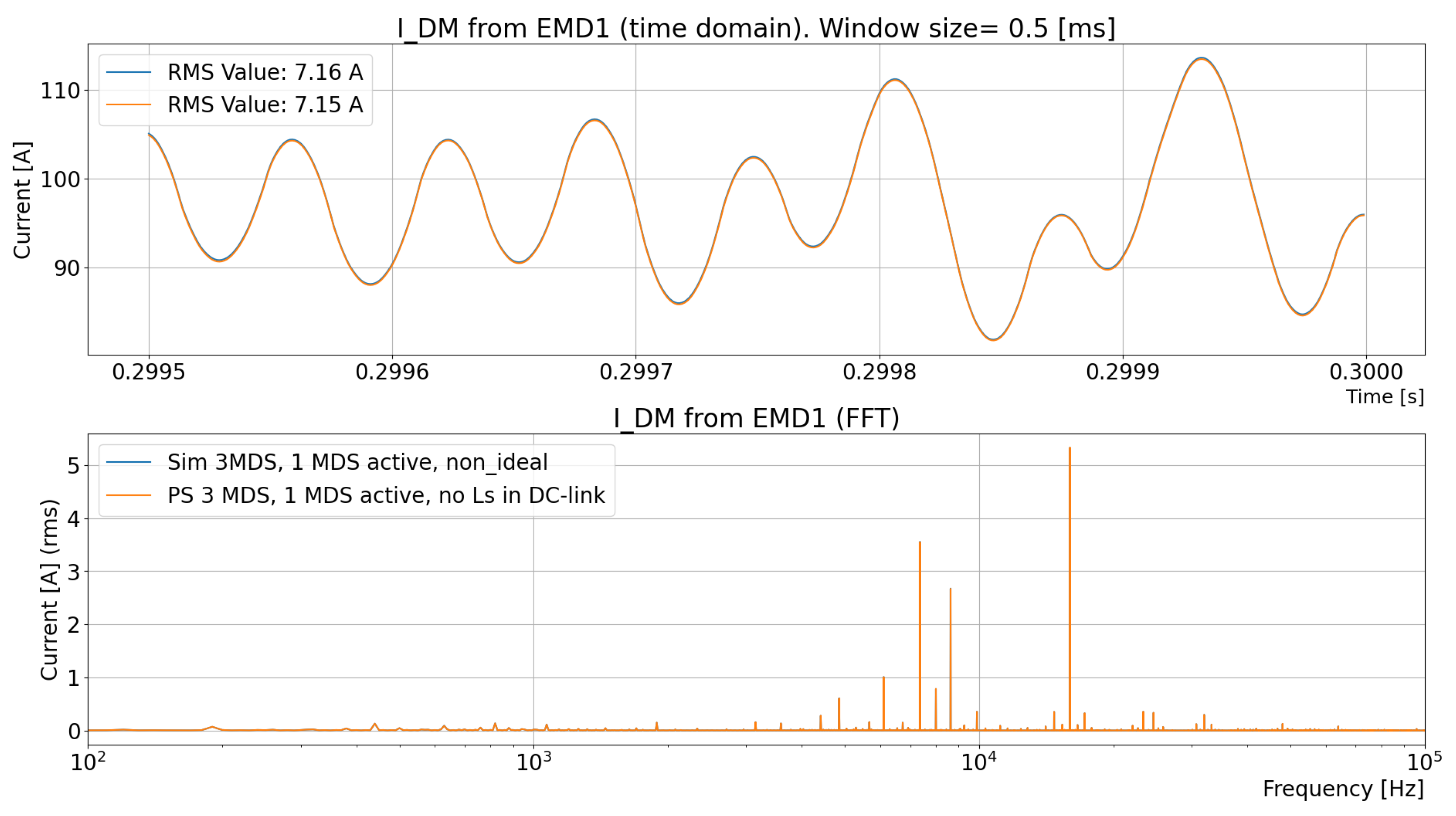
• The extended system model from step 3 is simulated again with a current source with the DC current drawn by the MDS from step 1; the MDS is replaced, and a slew rate is added to the DC-link current pulses. This model thus uses a more advanced system model but with an EMD behavior to account for the effects of the extended system model. The hypothesis is that these steps show the extent to which a complete MDS can be replaced by a current source with an adjustable slew rate. In these system simulations, the system simulation complexity and simulation time are significantly reduced; see Section 2.4.4. The results of the different simulation models in items 3 and 4 are compared.
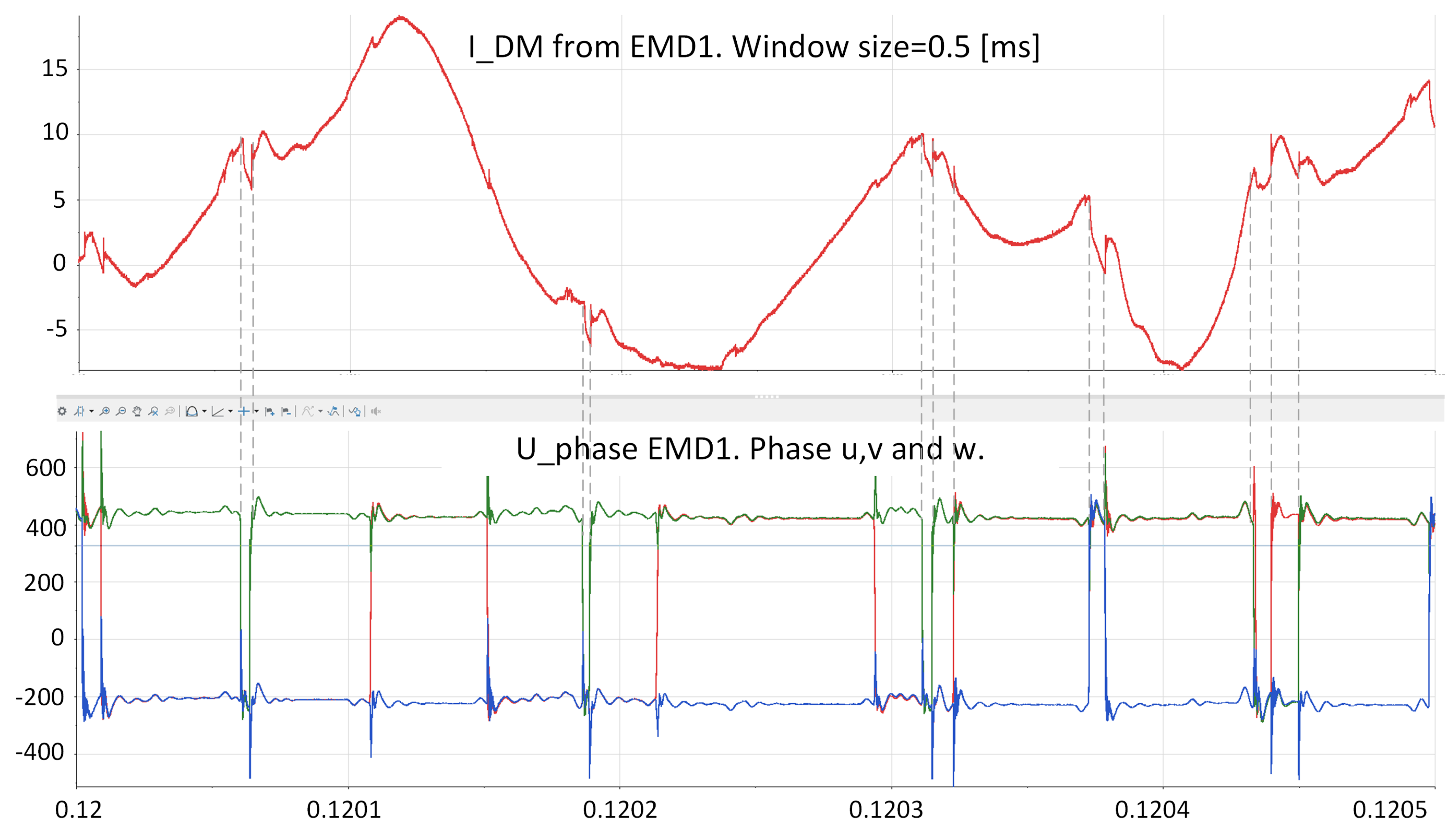
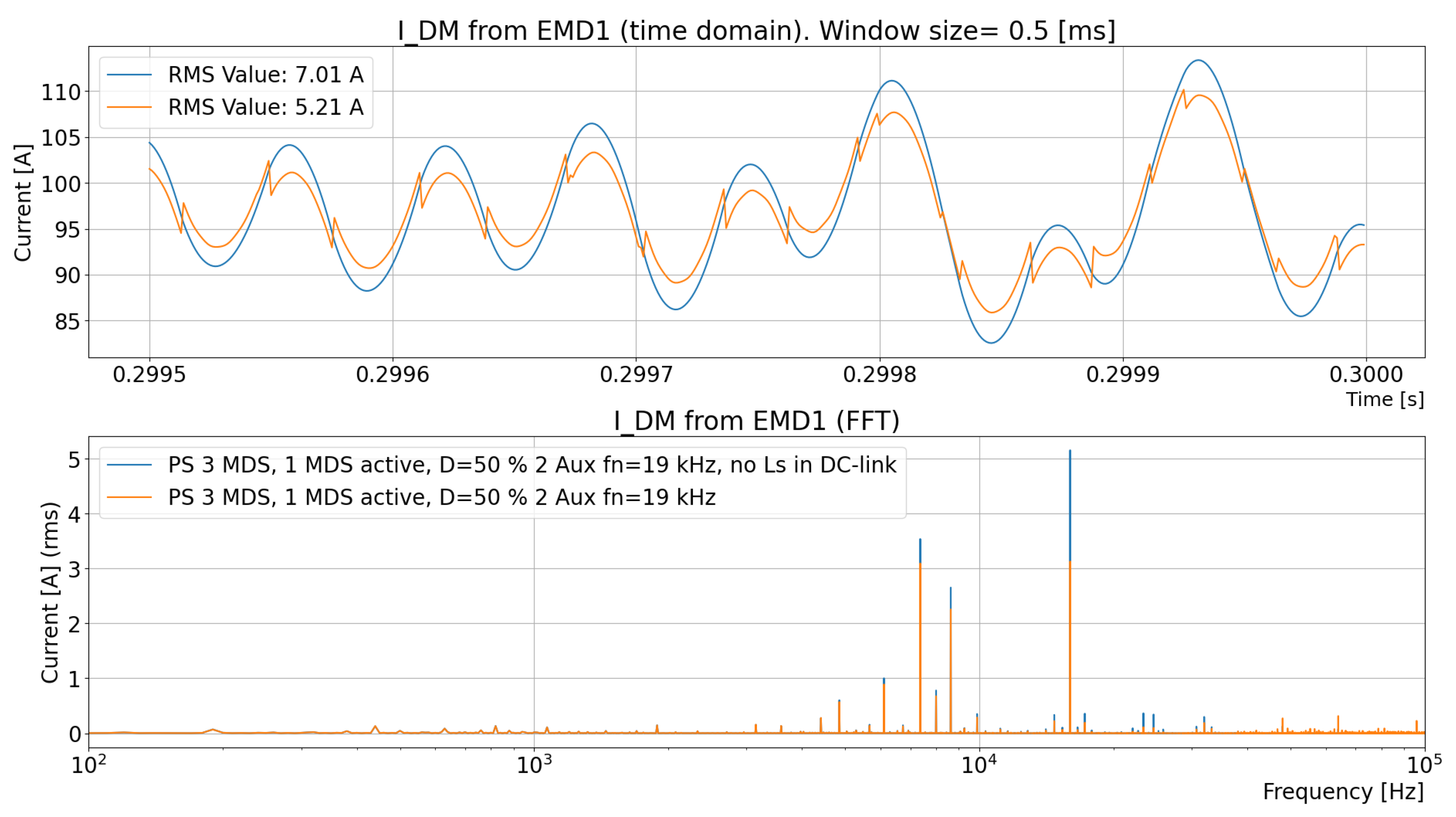
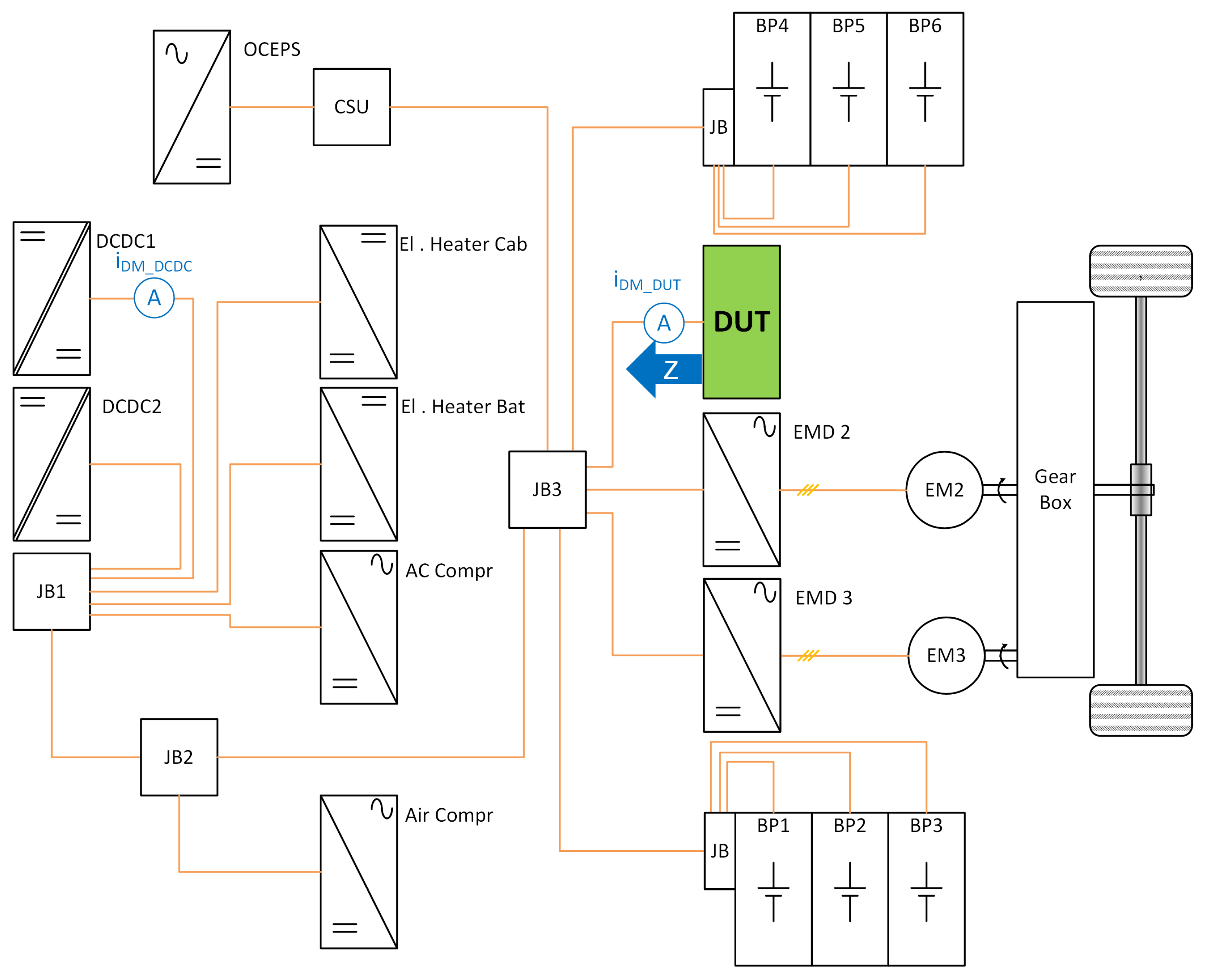
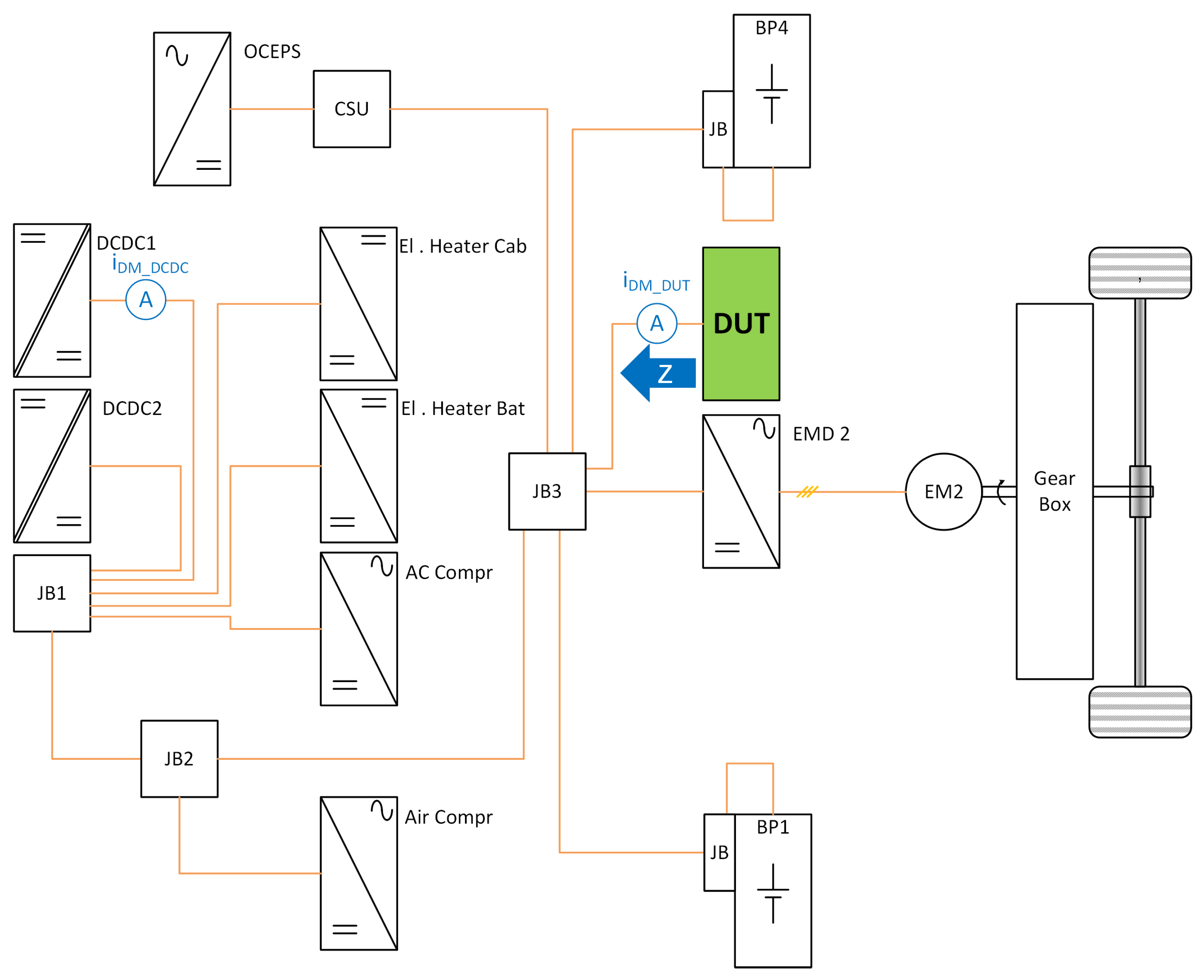
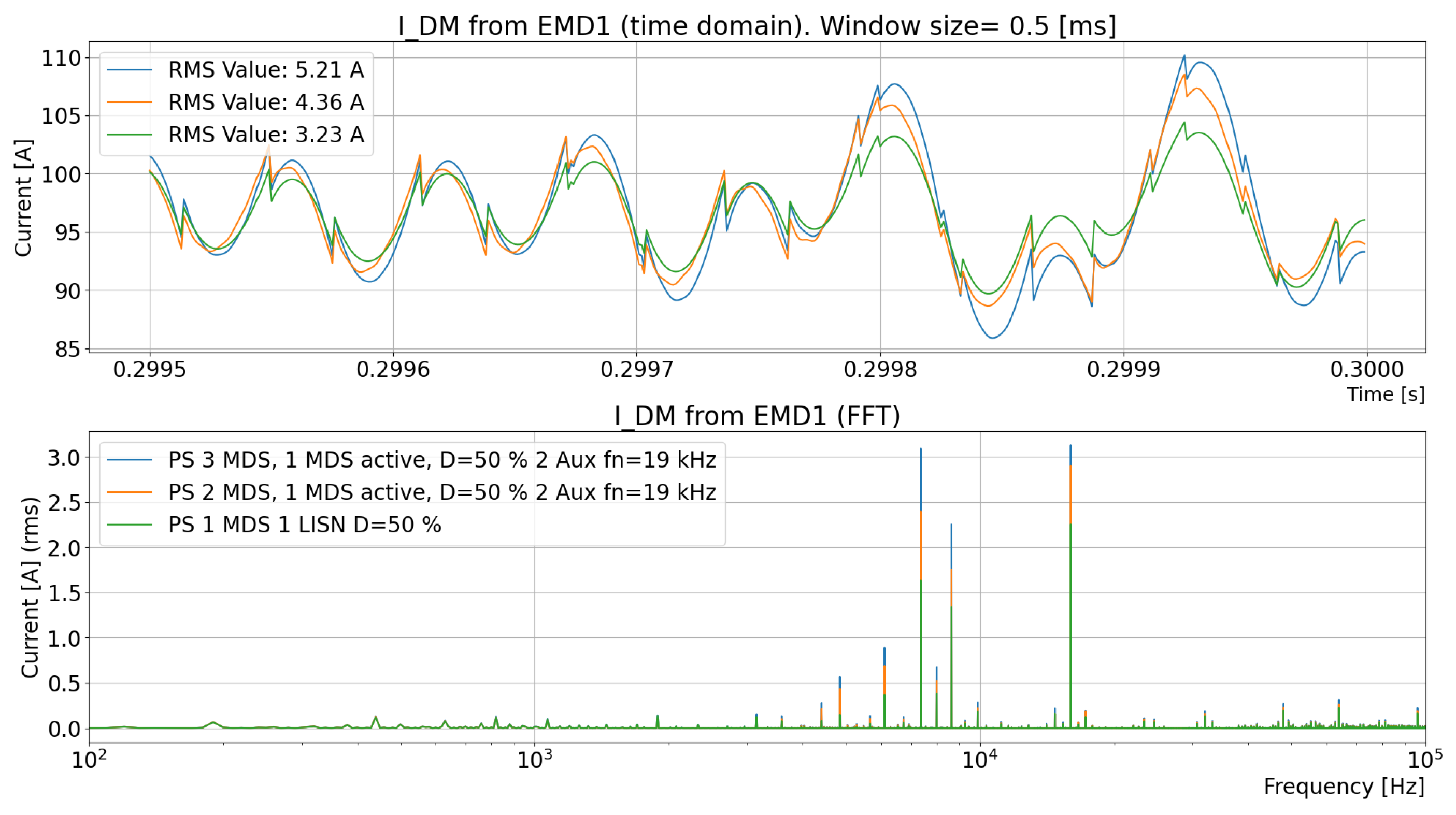
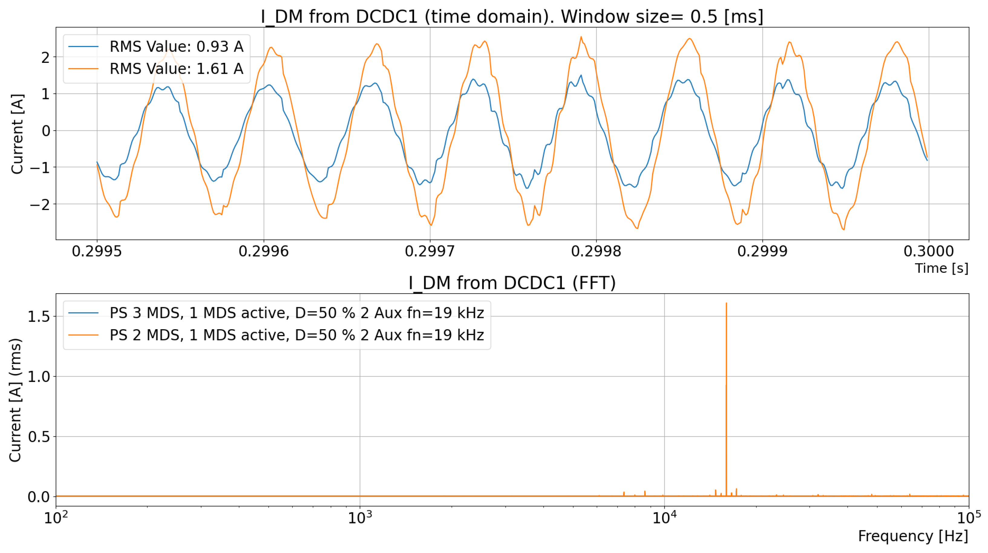
• The DC DM current to the EMD caused by the impact of the DC-link capacitor’s stray inductance is compared. This comparison involves a measurement from a real vehicle, as shown in Figure 1; see Section 2.4.5.
• A conclusion is drawn regarding items 1–5; see Section 2.4.6.

All cases simulated in Section 2.4 represent an operation point that is at half of the base speed combined with the maximum torque.

In Figure 8, Figure 9, Figure 10 and Figure 11, there are some signals and components whose parameters are clarified in

Table 2. Parameters for the simulations according to Figure 8.

Electrical Parameter	Description
$n_{ref}$	Reference speed to the control system
$T_{ref}$	Reference torque to the control system
$i_s$	Feedback of the three-phase current to the control system
$\Theta$	Feedback of the phase angle to the control system
$\omega$	Feedback of the electrical speed to the control system
$G_s$	Gate signal to the three-phase bridge from the control system.
$u_{DC}$	Feedback of the DC voltage to the control system, measured with a volt meter.
$i_b$	Current from the DC link to the three-phase converter, measured with an ampere meter and recorded to a file.
$i_{DM}$	Differential-mode current, measured on the DC side. Main parameter for the investigation.
$u_{DM}$	Differential-mode voltage, measured on the DC side. Main parameter for the investigation.
$R_{BAT}$	Serial resistance in the battery.
$L_{BAT}$	Serial inductance in the battery.
$R_C$	Serial resistance in the cable.
$L_C$	Serial inductance in the cable.
$R_L$	Serial resistance in the filter inductance in the EMD.
$L_L$	Serial inductance in the filter inductance in the EMD.
$C_{DC-link}$	DC-link capacitor; in ideal simulations, there is no $R_S$ or $L_S$.
$R_S$	Serial resistance in the DC-link capacitor.
$L_S$	Serial inductance in the DC-link capacitor.

.

2.4.1. Reduced System Model with a Complete MDS with Active Feedback Control

The model in Figure 8 is a reduced system model with a complete MDS with active feedback control, as in a physical EMD in a truck, from the box “MDS SW&Ctrl”. The IGBTs are ideal, e.g., instant turn-off and turn-on. There are no cables or stray inductance in the circuit. The current to the three-phase bridge $i_b$, as shown in Figure 8, is recorded to a file and is used in the next step; see Section 2.4.2.

2.4.2. Extended System Models Where the EMD Models Are Simulated with a Current Source and the DC Current Is Drawn by the MDS

The simulation model in Figure 9 is simplified from the model in Figure 8 regarding the control, three-phase bridge, and EM. These are now replaced by a current source, as shown in Figure 9. The current source is controlled by the recorded current $i_b$, as shown in Section 2.4.1. A rate limiter is used to achieve a current generated by the current source, and this represents the current slope as an IGBT with rising and falling time. In this simulation model, nonideal components are introduced; the DC-link capacitor has a stray inductance $L_s$, a serial resistance $R_s$, nonideal cables, and a series inductance in the battery. Subsystems with nonideal circuits are also added. Apart from the advantage of using a controlled current source with correct rising and falling times that can run with a nonideal DC-link capacitor, this simulation runs much faster in PLECS. However, the recorded current shown in Figure 8 is used to vary the configuration of the simulation model in Figure 9—for example, when the natural frequency $f_0$ in the auxiliary subsystem is varied.

This is the extended model for the simulations. It includes stray inductances and the subsystems to be analyzed.

2.4.3. Extended System Model with a Complete MDS with Active Feedback Control

A question is, of course, raised as follows: is the current to the three-phase bridge affected when the system is varied in terms of adding auxiliaries that, for example, may affect the DC-link voltage and, thus, via the MDS feedback loops, indirectly affect the current drawn? To make sure that there is no effect, another simulation model is built, with the control shown in Figure 8. In this simulation, cables and inductance are introduced, as shown in Figure 9; the only difference is that the DC-link capacitor is kept ideal, i.e., without serial inductance; see Figure 10.

The current to the three-phase bridge $i_b$ is not affected even though the system is varied; see Figure 12. It is thus shown that the DM current to the three-phase bridge $i_b$ is not affected even though the system outside the three-phase bridge in the MDS, cables, subsystems, and battery is changed from ideal to nonideal. This suggests that the influence of the feedback control of the MDS on the DM current to the three-phase bridge, $i_b$, is negligible.

2.4.4. Extended System Model from Section 2.4.3 Where the EMD Model Is Simulated with a Current Source with the DC Current Drawn by the MDS

It is important to make sure that the simulation results remain mainly unaffected by the differences between the simulation models in Figure 10 and Figure 11. This is achieved by comparing the DM DC current ($i_{DM}$) drawn by EMD1 (the upper one in Figure 10 and Figure 11) and the DM DC-link voltage ($u_{DM}$) across the DC-link capacitor of EMD1 (the upper one in Figure 10 and Figure 11). The comparison’s results are shown in Figure 13 and Figure 14.

The simulation shows that both models give the same results for both current and voltage, which ensures that a model with recorded current can be used.

2.4.5. Comparing the Simulation Models with Measurements

In this subsection, a comparison is made between measurements from a truck and two simulation models with respect to the DC DM current dependence of the stray inductance in the DC-link capacitor. The DM current is measured on the DC side of EMD1. The voltage is measured on the AC side of EMD1. It is important to know how the current looks when the simulation models are built to make sure that the simulations and reality show similarities. The following graphs show the current in comparison with the phase potential. In Figure 15, the DM current on the DC side of EMD1 and the phase potential relative to the chassis of EM1 are shown.

In Figure 15, it is shown that the DM current is affected when the EMD switches. A simulation is performed, and a comparison is made with and without the stray inductance $L_s$ in the DC-link capacitor (see Figure 9 and Figure 16).

Comparing Figure 15 and Figure 16, it is clear that the “notch in the curve” seen in the top graph in Figure 15 can also be seen in the top graph in Figure 16 for the orange curve, which includes the stray inductance in the DC-link capacitor.

2.4.6. Conclusion for the Simulation Model

In Section 2.4, a comparison of the following is performed:

• MDS with active feedback control and MDS replaced by a controlled current source;
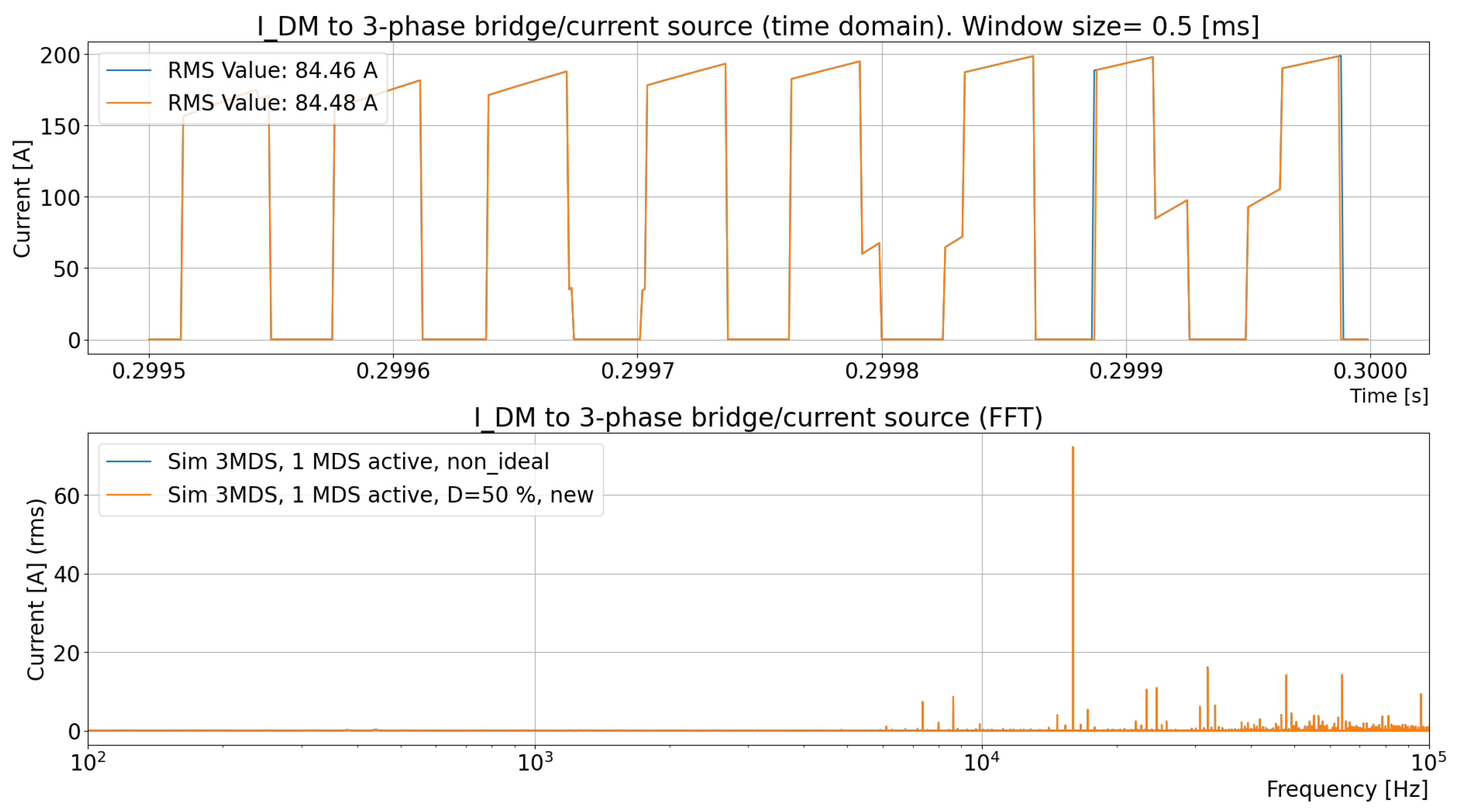
• The DM current to the three-phase bridge, $i_b$, when the system uses ideal vs. nonideal components or additional subsystems.
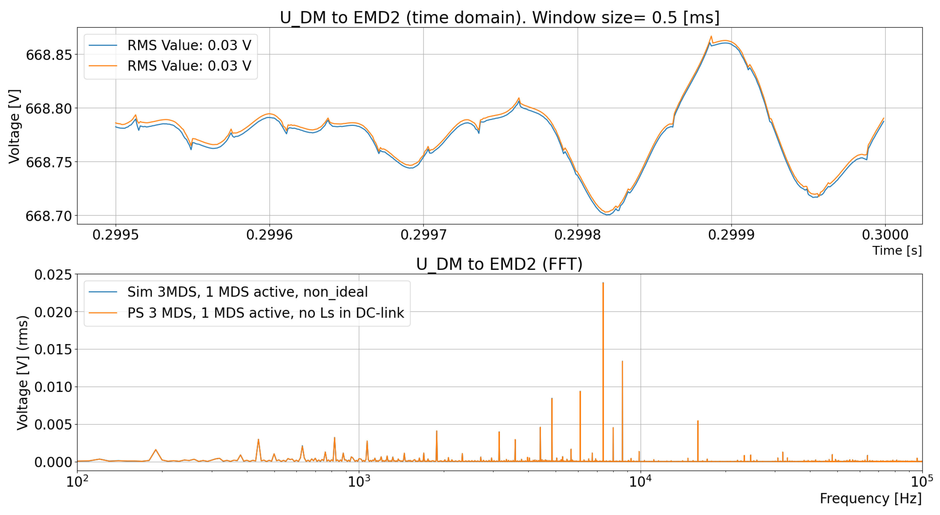
• Excluding or including the stray inductance $L_s$ in the DC-link capacitor.

The comparison demonstrates the following:

• A simulation model with a controlled current source, from the recorded current to the three-phase bridge $i_b$, can be used.
• The current to the three-phase bridge, $i_b$, is independent if the system changes, as demonstrated in this study.
• The stray inductance in the DC-link capacitor, $L_s$, cannot be omitted if the DM DC-link voltage, $u_{DM}$, should be properly modeled.

2.5. Line Impedance Stabilization Network (LISN) Model in PLECS

A complete electric vehicle should be tested in terms of the voltage and current ripple in the connection point of a subsystem to the TVS. When a prototype vehicle is built, the time until the start of production is limited. A way to verify the included subsystems in an early phase is necessary. An artificial network, also known as a line impedance stabilization network (LISN), is a standardized method of EMC testing for conducted and radiated emissions. An artificial network is described in [22]. The purpose of the LISN is to define a standardized input impedance to the DUT for repeatable tests. The input impedance is marked with “Z” in Figure 17 for the DUT with an LISN. A quote from [22] is “This test describes a standardized test setup and test method to enable comparability of the generated voltage ripple of voltage class B components”.

An artificial network is used for the generated ripple test, as shown in Figure 17.

The LISN, according to [22], is shown in Figure 18.

$R_{i,HV}$, Internal resistance of the power supply.

$L_V$, Internal inductance of the vehicle—mainly of the vehicle power supply and cables.

$C_Y$, Capacitor between HV+/HV− and the ground to limit EMC.

$C_s$, Decoupling capacitor.

2.6. Characteristics of a TVS

The aim of using an LISN is to foresee disturbances that occur when operating a TVS. A TVS includes batteries, converters, and cables of different designs and configurations. The main properties of these are the following:

• Battery: Ideal voltage source, internal resistance, CM and DM inductance, and CM parasitic capacitance towards the ground.
• Converter: DC-link capacitance, filter inductance, and CM capacitance $C_Y$.
• Cables: Resistance and inductance.

The properties of the TVS form different impedance and resonance circuits.

To compare the difference in the impedance between two differently configured vehicles, a frequency sweep of the simulation model is performed. Both models are equipped with the same auxiliary loads but different numbers of batteries and electrical machine drives. The vehicle shown in Figure 1 is a reference to show the difference in impedance of system changes. A test is performed where EMD1 is removed and replaced with a DUT, and the TVS is investigated for the perceived impedance from the perspectives of both the DM and CM. The large vehicle configuration is shown in Figure 19, and the smaller vehicle configuration is shown in Figure 20.

In the simulation model, the inner impedance of the TVS is marked with “Z” in Figure 19 and Figure 20 in the connection point of the DUT. The retrieved impedance Z from the simulation in PLECS for the DM is shown in Figure 21 and for the CM in Figure 22.

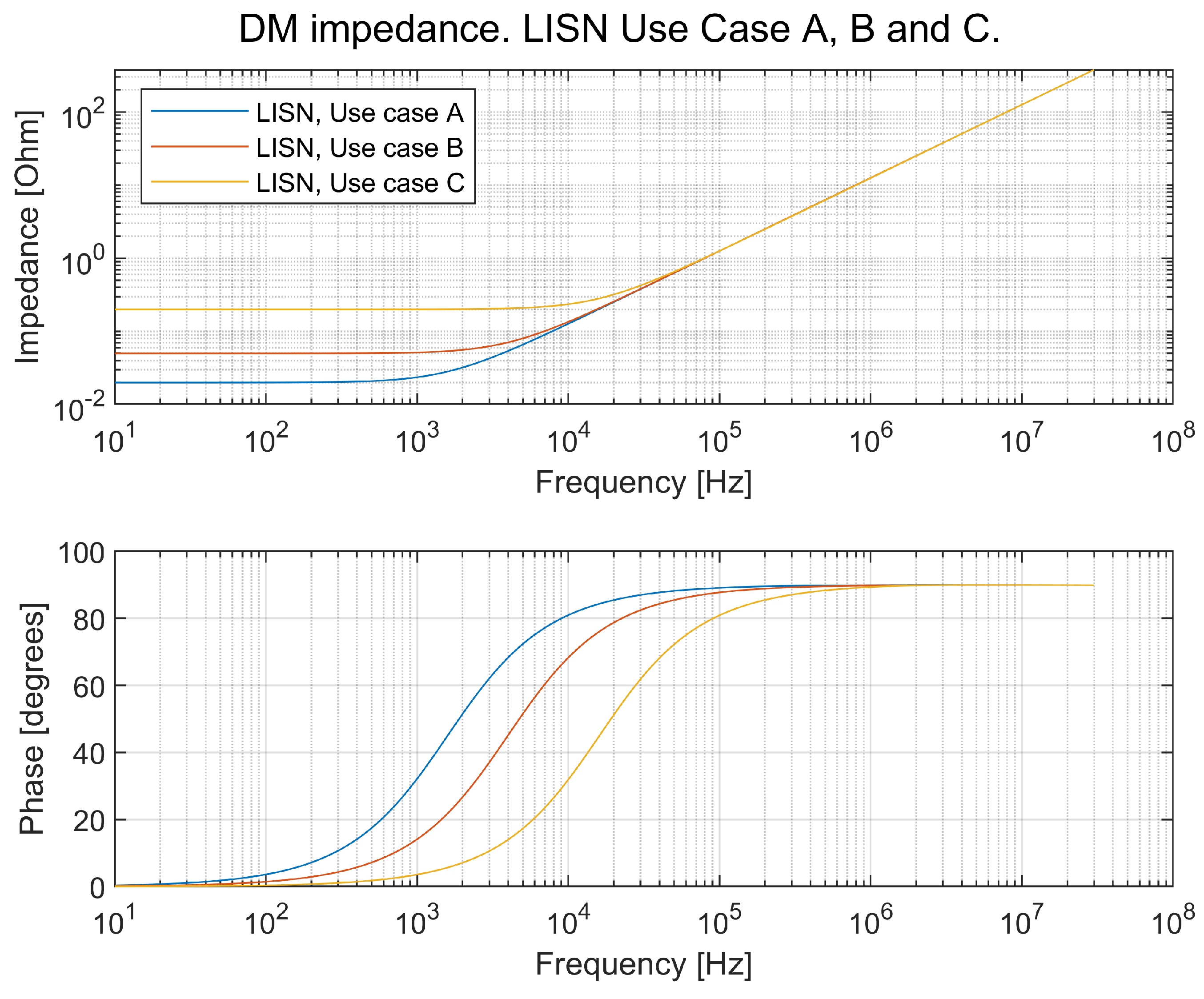
2.7. Characteristics of an LISN

An LISN is shown in Figure 18. According to [22], there are four different use cases for an LISN; the internal resistance in a high-voltage power supply is varied in three of the use cases, and one use case is free for agreement with the customer and supplier. The parameters referring to Figure 18 are given in

Table 3. Use cases from Annex D in [22].

Use Case	${\mathit{R}}_{\mathit{i},\mathit{H}\mathit{V}}$ [m$\mathsf{\Omega }$]	${\mathit{L}}_{\mathit{V}}$ [$\mathsf{\mu }$H]	${\mathit{C}}_{\mathit{Y}}$ [$\mathsf{\mu }$F]
A	10	1	1
B	25	1	1
C	100	1	1
Z	To be agreed between customer and supplier.	To be agreed between customer and supplier.	To be agreed between customer and supplier.

.

$C_S$ shall be 10 mF or greater according to [22]. It should be noted that 10 mF is a large capacitance compared with the DC-link capacitance of the vehicle in this study. The impedance over the frequency for use cases A–C in Figure 17 is shown in Figure 23 for the DM impedance and in Figure 24 for the CM impedance.

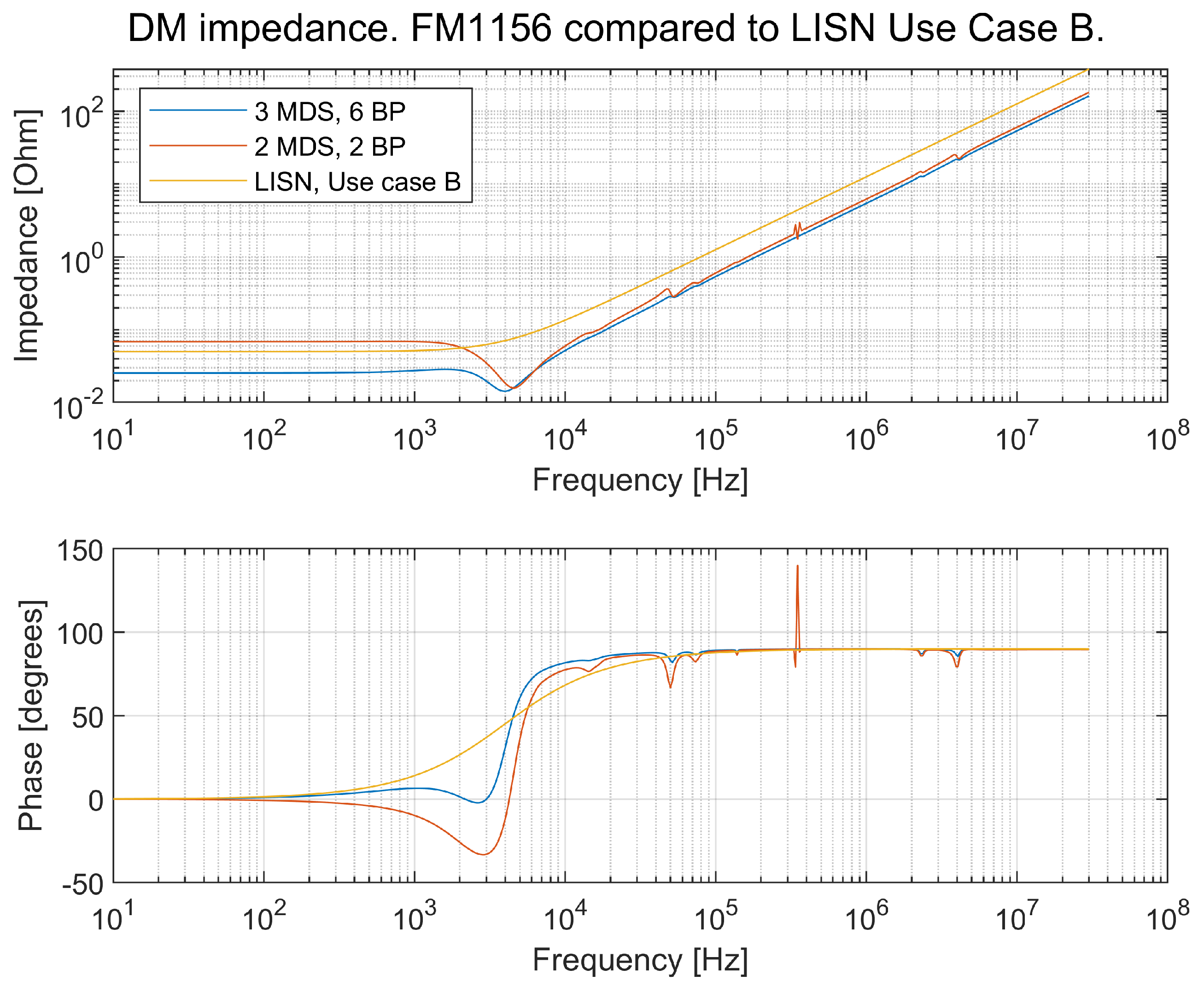
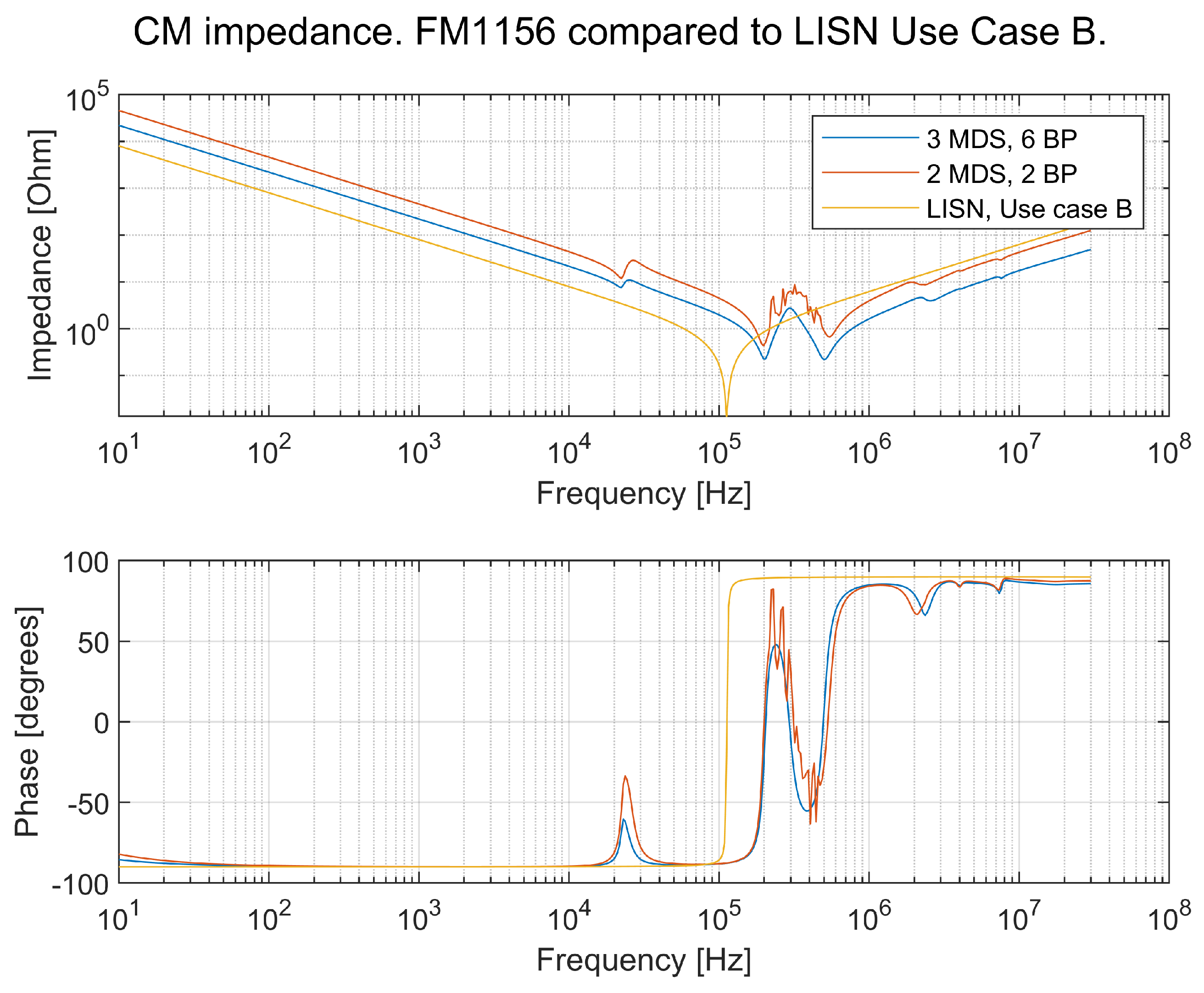
2.8. Impedance Comparison of an Artificial Network, an LISN, and Measurements on a Real Truck

The DUT is a component that is planned to be included in a vehicle. The behavior of the DUT and the LISN shall reflect how the DUT behaves in the vehicle. A frequency sweep of three different models reflecting the inner impedance of the following:

• The input impedance “Z” to the TVS as seen from the DUT of the vehicle (see Figure 19) with three MDSs and six BPs;
• The input impedance “Z” to the TVS as seen from the DUT of the vehicle (according to Figure 20) with two MDSs and two BPs;
• The input impedance “Z” to the TVS as seen from the DUT of the LISN (see Figure 17) using case B, as shown in Table 3,

is shown in Figure 25 and Figure 26 for the DM and CM, respectively.

It can be seen in Figure 25 and Figure 26 that the input impedance—perceived from the DUT—differs for both the DM and CM between the small and large vehicles, but it differs even more between the vehicle models and the LISN. At a frequency of around 4–6 kHz, there is a distinct resonance frequency in the vehicle model. However, there are more resonance frequencies that are not as distinct as this one.

In conclusion, the LISN does not reflect the TVS, and the development of an alternative LISN is recommended. It is proposed that OEMs develop a few variants of LISNs to be used by suppliers to better reflect the vehicles in which subsystems will be used. As of today, LISNs do not reflect the conducted emissions.

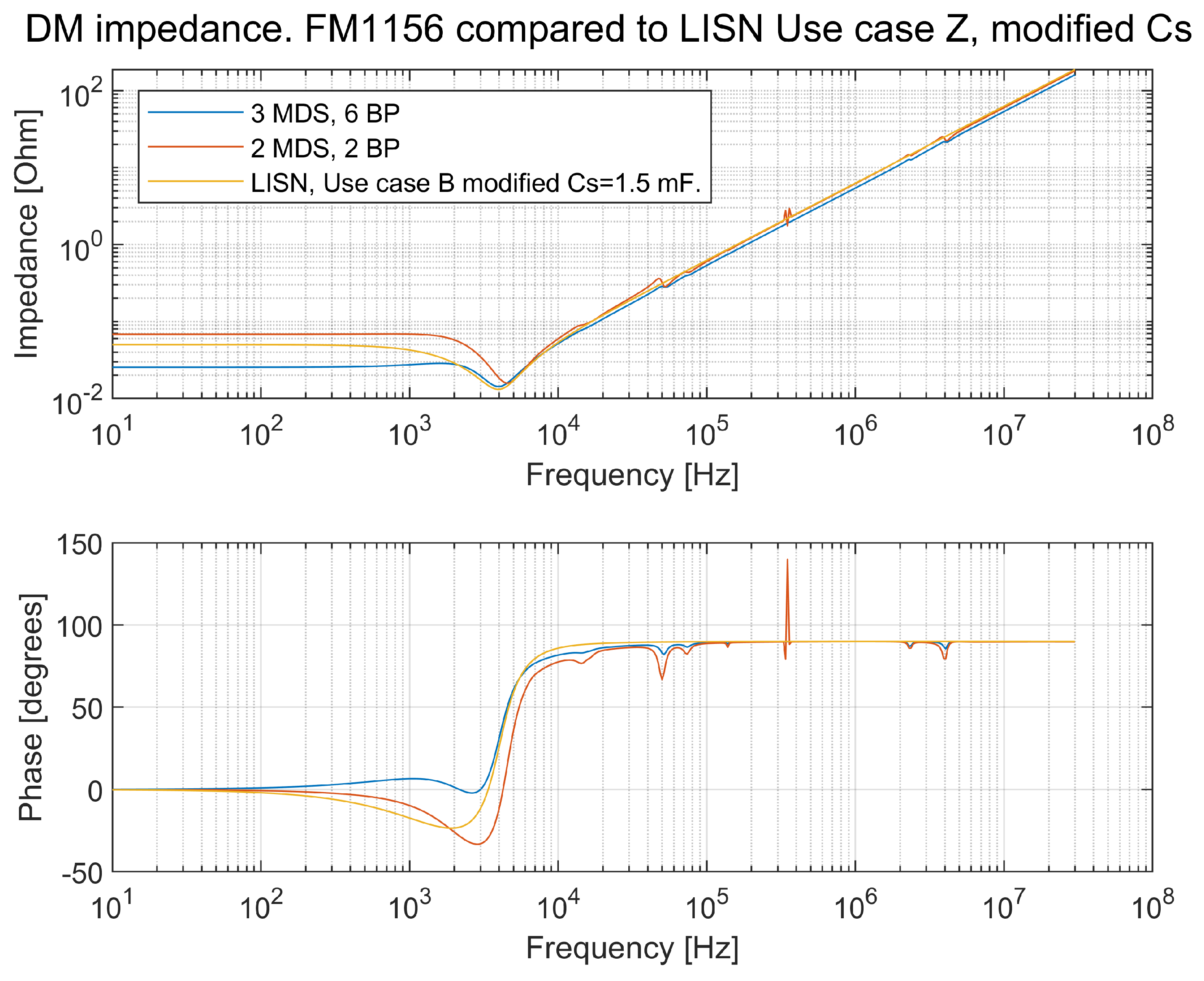
2.9. Alternative LISN

In Section 2.8, it was found that the LISN does not sufficiently represent the TVS of a vehicle in the connection point of a subsystem. The LISN should reflect all kinds of loads that are connected to the TVS, such as batteries and converters. The characteristics of a battery from the perspective of the DM are a voltage source with serial resistance and inductance. For low frequencies, there is a resistive impedance, and there is an inductive impedance for higher frequencies; see Figure 9. A converter mainly has a DC-link capacitor as the impedance for low frequencies and the stray inductance in the DC-link capacitor and CM inductor in the input for higher frequencies; see Figure 9. The LISN does not show any resonance frequency, as $R_{i,HV}$ in Figure 18 has a “high” resistance and eliminates the low impedance at the resonance frequency. One way to avoid this is to move the decoupling capacitor (see Figure 17) between $L_V$ and $R_{i,HV}$ (see Figure 27). Moving $C_S$ is, however, not according to the use case and test setup shown in Figure 17.

A comparison of the DM and CM impedance between the LISN and the modified LISN is shown in Figure 28 and Figure 29, respectively.

The DM impedance for the modified LISN looks better with one resonance point. The CM impedance looks the same for the standardized LISN as it does for the modified LISN. According to Table 3, use case Z admits that all three parameters can be changed to agree with the customer. Still, only one resonance circuit is formed. Changing $L_V$ forms the impedance after the resonance point. $L_V$ is changed to correlate to the vehicle, and $C_S$ is also changed to a value that provides conformity with the vehicle model. Changing and moving $C_S$ is, however, not according to the use case and test setup shown in Figure 17. A comparison between the modified LISN with changed values of $L_V$ and $C_S$ and the vehicle is shown in Figure 30.

It can be seen in Figure 30 that the alternative LISN better reflects the impedance of the TVS.

2.10. Protecting Subsystems from EMI

A TVS can contain subsystems from different suppliers. One thing that will help the subsystems from disturbing each other is an input filter. Some suppliers offer CM filters for the input, but they seldom offer a DM filter. Three different input filters are shown in Figure 31:

L, DM filter inductor;

C, DC-link capacitor;

$R_d$, Damping resistor;

$L_d$, Damping inductor;

$C_d$, Damping capacitor.

The filter inductor L can be a pure DM inductance or the stray inductance in a CM inductor. When it is the stray inductance, the inductance is low. The design of the LC filter is shown in [23]. The input impedance of the LC filter in a serial damped filter and a parallel damped filter is shown in Figure 32. The transfer functions of the same filters are shown in Figure 33.

It is obvious in Figure 33 that a damped filter is preferable to an undamped LC filter. A TVS is built from many subsystems and, according to Figure 1, there can be seven different resonance circuits, one for each subsystem. Imagining that all of them are undamped, the risk of triggering a resonance is severe.

In the example in Figure 33, the DM inductance is only stray inductance from a CM inductor. Imagine that a subsystem with an undamped LC filter is moved around in a vehicle. A simulation with three different configurations is conducted (0 m of cable, 1 m of cable and one JB, and 10 m of cable and three JBs). The transfer function is shown in Figure 34.

It can be seen in Figure 34 that the resonance frequency is changed from 20.4 kHz with 0 m cable length down to 17.5 kHz with 10 m of cable and three JBs. The conclusion from this is that when the converter is moved from one installation to another, the resonance frequency changes. The effect is that the EMI can be severely changed.

The same comparison for a parallel damped circuit is shown in Figure 35.

It can be seen in Figure 35 that the effect of moving the converter around is minor.

Conclusion: To build a stable platform, it is necessary to make sure that the subsystems have a DM filter on the input to mitigate the risk of resonances. Harmful resonances can be triggered when a switching frequency is changed or when a subsystem is moved in the installation. It is the responsibility of the OEM, who is responsible for the TVS to define this cut-off frequency, and it is the responsibility of the sub-supplier to design the filter.

3. Results

3.1. Results from a Simulation of a Truck Model Compared with an LISN

A comparison of the differential-mode current from the EMD, $i_{DM\_EMD}$, in a simulation model of a large truck configuration (three EMDs and six batteries; see Figure 19), small truck configuration (two EMDs and two batteries; see Figure 20), and a model of the LISN (use case B; see Figure 17 and Figure 18 and Table 3) is shown in Figure 36 (references are made to currents in Figure 1).

It is found that the RMS current of $i_{DM\_EMD}$ is

84% for the small configuration compared with the large configuration of the truck. Additionally, it is

62% for the LISN simulation vs. the truck model.

It is concluded that the difference in the differential-mode RMS current of $i_{DM}$ between the small and large configurations is less than the difference between the truck models and the LISN. An alternative LISN is required to better reflect the vehicle.

However, what happens within the TVS?

3.2. What Happens Inside the TVS That Is Not Observed with the LISN?

An observation of the DM current to the DC/DC converter $i_{DM\_DCDC}$ in a simulation model of a large truck configuration (three EMDs and six batteries; see Figure 19), small truck configuration (two EMDs and two batteries; see Figure 20), and a model of the LISN (use case B; see Figure 17 and Figure 18 and Table 3) is shown in Figure 37 (references are made to currents in Figure 1).

It is found that the RMS current of $i_{DM\_DCDC}$ to the DC/DC converter is 173% for the small-configuration truck vs. the large-configuration truck. An important conclusion is that switching frequencies and natural resonance frequencies must be taken care of.

Another comparison is made between two large-configuration trucks where the difference is that the natural resonance frequency for the DC/DC is changed from 19 kHz to 8 kHz. The DM current to the DC/DC for the two configurations is shown in Figure 38.

It is found that the RMS current of $i_{DM\_DCDC}$ to the DC/DC converter is 344% for DC/DC with the resonance frequency of 19 kHz with respect to that with 8 kHz.

This large change is, however, not reflected at all in the DM current of $i_{DM\_EMD}$ to EMD1, as shown in Figure 39.

It is found that the RMS current of $i_{DM\_EMD}$ to the EMD1 converter is 99% for DC/DC with a resonance frequency of 19 kHz compared with that with a frequency of 8 kHz. An important conclusion is that changes in the included auxiliary components result in large changes in the current within the TVS, which cannot be seen in the EMD DM current and, thus, not in an LISN simulation.

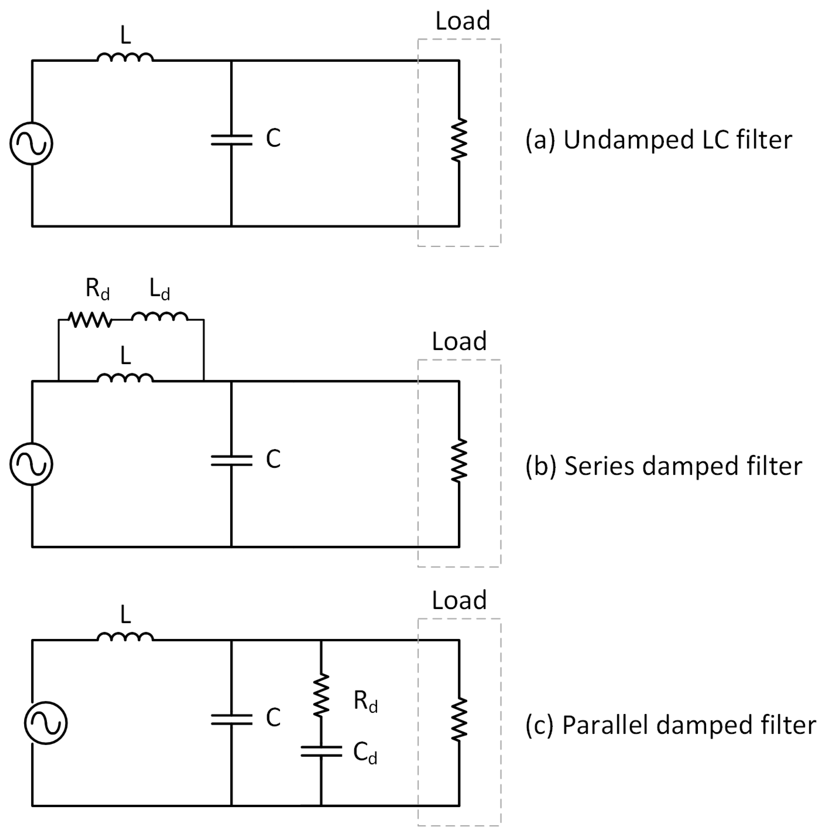
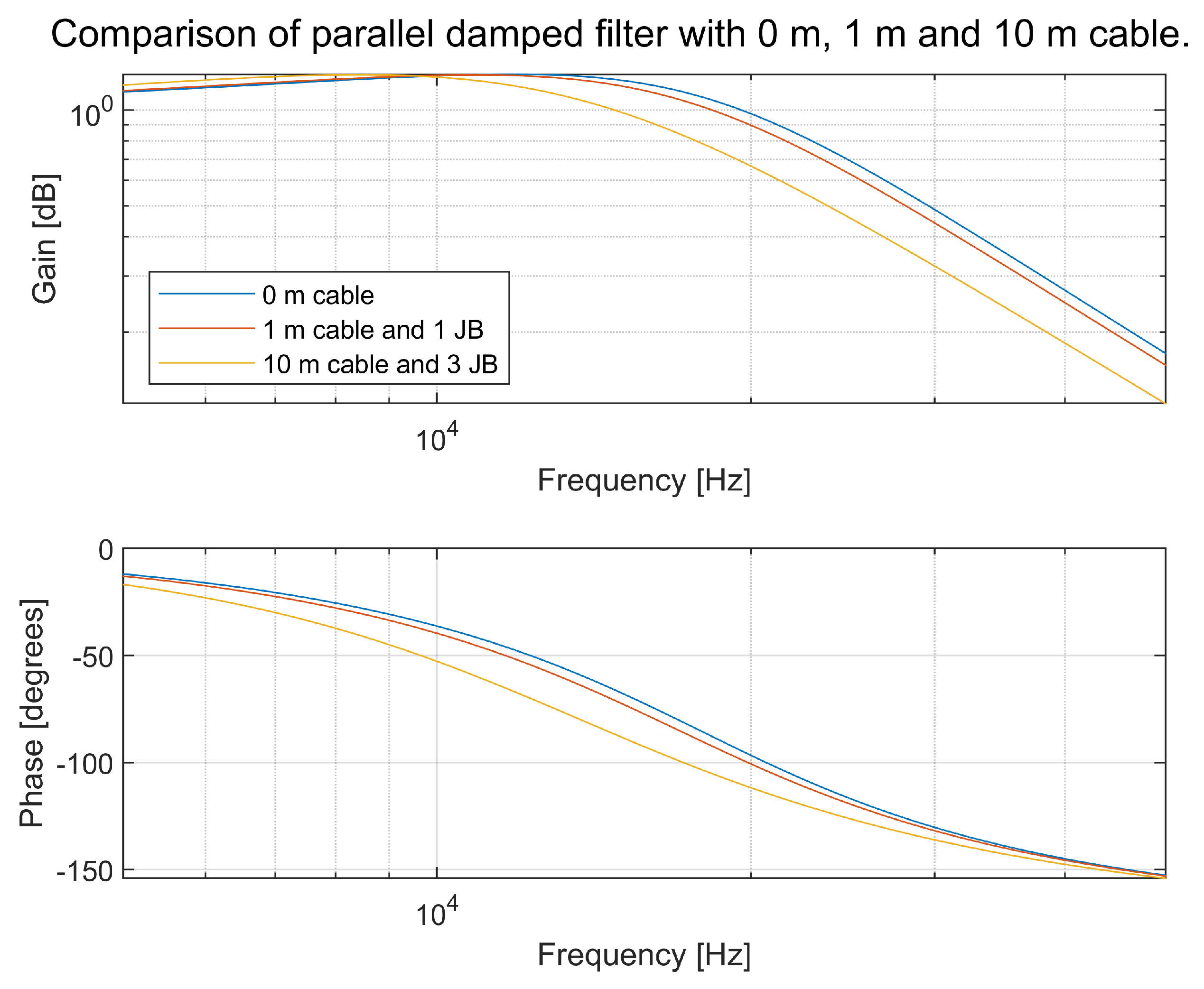
3.3. Damped Filters in the Subsystems

One of the auxiliary components, the DC/DC converter, is equipped with damped filters in this subsection with reference to Figure 31, resulting in a lower current ripple. The conducted differential-mode ripple current caused by the neighboring EMD1 is shown in Figure 40.

It is found that the RMS current of $i_{DM\_DCDC}$ to the DC/DC decreases to $36\%$ for the serial damped filter and $31\%$ for the parallel damped filter compared with the undamped filter. The important takeaway is that a subsystem shall protect itself from resonances triggered by neighboring subsystems. In a large TVS, such as a commercial BEV, it is hard to foresee all of the characteristics of the included subsystems, including characteristics such as resonance frequencies and switching frequencies.

The effect on the differential-mode current from the EMD, $i_{DM\_EMD1}$, is minor when the filter changes in the DC/DC; see Figure 41.

4. Discussion

The expanding market for commercial electric vehicles requires fast and safe development. The platform for development should be robust. A robust platform is, among other properties, one in which subsystems can be combined in various combinations and placed at different locations onboard a vehicle, e.g., with varying lengths of cables. The switching frequencies and natural frequencies cannot be left to their own destiny. Many subsystems are available as off-the-shelf components. It is of the highest importance that a complete traction voltage system is investigated in terms of switching frequencies and natural resonance frequencies. Either all subsystems should have natural frequencies “far from” switching frequencies or all subsystems should protect themselves from resonances, e.g., by being equipped with damped filters. A line impedance stabilization network (LISN)/artificial network, as validation that a new subsystem will work on a platform, cannot be used without a combination of simulations and/or measurements of the complete system. The exact values and percentage differences in this article are not important; the important takeaway is to reflect on how the subsystems impact each other.

A natural question to ask is when a simplification of a simulation model is enough, or too much, to properly replicate the events in a real TVS and in the frequency range of interest. It is mathematically possible to quantify a difference between a measured quantity and the simulated equivalent by means of, e.g., a quadratic average, and then to set a maximum allowed value for that difference. However, measured quantities are very hard or even impossible to replicate in simulations, since the measurements are made on a full system consisting of many independent subsystems with unknown (sub-supplier proprietary information) power-electronic control.

It is the opinion of the authors that such a procedure is insufficient and still leaves a need for a subjective visual inspection of the waveforms. It is also the opinion of the authors that the exact values and relative differences in this article are less important; the important takeaway is to reflect on how the subsystems impact each other.

5. Conclusions

This article focuses on the modeling and simulation of an electric traction voltage system (TVS) in a road vehicle, such as a heavy-duty truck, with respect to the DM EMI while including all relevant subsystems. This is necessary to facilitate the understanding of current systems and to set requirements for future systems. It is argued that the ability for detailed modeling and simulation is essential and that a complete circuit simulation model needs to represent frequency components for the DM of up to at least 100 kHz and for the CM of up to at least 1 MHz. It is recognized that detailed system simulation models become too large for practical use and that model reduction methods are needed. This article presents such model reduction methods and discusses how these reduced models perform in comparison with the use of a generalized artificial network/line impedance stabilization network (LISN). The article also shows that the use of DM filters on the TVS terminals of the subsystems significantly improves the TVS’s stability against different system configurations.

With the proposed practically functional reduced simulation model, robust, cost-effective, and time-saving development can be achieved. In particular, the following conclusions are drawn.

5.1. Conclusions from the Development of the System Simulation Model

A method for mitigating the constraints of a full simulation model (representing all known circuit elements and feedback loops) is to replace the DC-link current drawn by the power-electronic converter, $i_b$ in Figure 8 and Figure 10, in a traction machine drive with a corresponding current source, as shown in Figure 9 and Figure 11. This is achieved by recording the DC-link current drawn by a detailed subsystem model using ideal switches and replacing the full converter and related feedback loops with the recorded DC current as a current source with a slew rate corresponding to $t_{on}$/$t_{off}$ of the real transistors. This eliminates the need to represent the switching dynamics, which are very time-consuming to simulate, in a full TVS, and it facilitates the simulation of a few seconds of real time with a complete TVS in a reasonable working time. It is shown that, from the perspective of EMC/EMI in the frequency range of interest, this simplification introduces insignificant changes in the DM TVS current drawn by the modeled subsystem and, thus, simplifies and accelerates system studies.

5.2. Conclusions from Simulations with the LISN

The use of an LISN is a standardized way to test subsystems according to [22]. For traction voltage systems (TVSs) in commercial electric vehicles, the research presented here shows that the LISN’s impedance does not represent the impedance of a TVS well enough. There is a larger difference in the simulated DM current drawn from the TVS by an MDS between the LISN and the reduced TVS model than between a large (six batteries, three traction machines) and small TVS (two batteries, two traction machines) in a fully electric heavy-duty truck. A change in switching frequency when using an LISN may not show any differences at all. Inside a TVS, a resonance can be triggered, and high currents can flow between subsystems, which is not seen when using the LISN. The resonance can shorten the lifespan of the affected subsystems. The LISN also only represents a voltage source and cables. The low impedance of a neighboring converter’s DC-link capacitor is not reflected, nor are all of the different resonances in the TVS. An alternative LISN should be considered, but this should still be in combination with simulations and measurements of complete TVSs.

5.3. Conclusions from the DM Filters

Using differential-mode filters at the input of the subsystems mitigates the risk of triggering high-resonance currents. As traction voltage systems differ between installations in trucks, the resonance frequency may vary due to different cable lengths or different combinations of subsystems. The DM filter minimizes the risk of high-resonance currents. Figure 40 shows that the DM current drawn from the TVS by a subsystem current is significantly lower with a DM filter when a resonance frequency is triggered. The use of DM filters ensures the development of a stable platform that includes several configurations of a number of MDSs, ESSs, and other subsystems.

5.4. Recommendations for Future Research

The work presented here is confined to modeling a TVS with its subsystems. Thus, it does not include the additional systems related to connection to external systems, such as another vehicle (V2V, vehicle-to-vehicle) or an external AC grid for charging (G2V, grid-to-vehicle) or discharging (V2G, vehicle-to-grid). With those systems added, the circuit to simulate grows even further, as does the need for model reduction. The presented methods for model reduction are applicable to such circuit expansions.

Another future research subject is to investigate whether it is possible to develop an alternative LISN that represents a complete traction voltage system with respect to internal resonances in and between subsystems. The proposed reduced system simulation methodology is suitable as a benchmark for the development of such an LISN.

References

1. Schiedermeier, M.; Rettner, C.; Heilmann, M.; Schneider, F.; März, M. Interference of automotive HV-DC-systems by traction voltage-source-inverters (VSI). In Proceedings of the 2019 IEEE Transportation Electrification Conference, ITEC-India 2019, Bengaluru, India, 17–19 December 2019. [Google Scholar] [CrossRef]
2. Gürlek, Y.; Joos, O.; Lang, C.; Ackerl, M.; Dold, R.; Basler, T.; Neuburger, M. Analysis on the Impact of Current Ripples in Fuel Cell Electric Heavy-Duty Trucks. In Proceedings of the 2023 25th European Conference on Power Electronics and Applications, EPE 2023 ECCE Europe, Aalborg, Denmark, 4–8 September 2023. [Google Scholar] [CrossRef]
3. Lee, Y.H.; Nasiri, A. Conductive CM and DM noise analysis of power electronic converters in electric and hybrid electric vehicles. In Proceedings of the VPPC 2007—Proceedings of the 2007 IEEE Vehicle Power and Propulsion Conference, Arlington, TX, USA, 9–12 September 2007; pp. 392–398. [Google Scholar] [CrossRef]
4. Gentejohann, M.; Schluter, M.; DIeckerhoff, S.; Hepp, M. Driving Cycle Analysis of the DC Bus Current Ripple in Electric Vehicles. In Proceedings of the 2021 23rd European Conference on Power Electronics and Applications, EPE 2021 ECCE Europe, Ghent, Belgium, 6–10 September 2021. [Google Scholar] [CrossRef]
5. Wang, K.; Lu, H.; Li, X. High-Frequency Modeling of the High-Voltage Electric Drive System for Conducted EMI Simulation in Electric Vehicles. IEEE Trans. Transp. Electrif. 2023, 9, 2808–2819. [Google Scholar] [CrossRef]
6. Gentejohann, M.; Schlueter, M.; Dieckerhoff, S. Investigation of the Current Ripple caused by the Main Inverter in the High Voltage DC Bus of Electric Vehicles. In Proceedings of the VCIPS 2020; 11th International Conference on Integrated Power Electronics Systems, Berlin, Germany, 24–26 March 2020; Available online: https://ieeexplore.ieee.org/document/9097687 (accessed on 29 January 2025).
7. Aguirre, M.; Madina, P.; Poza, J.; Aranburu, A.; Nieva, T. Analysis and comparison of PWM modulation methods in VSI-Fed PMSM drive systems. In Proceedings of the 2012 20th International Conference on Electrical Machines, ICEM 2012, Marseille, France, 2–5 September 2012; pp. 851–857. [Google Scholar] [CrossRef]
8. Bierhoff, M.H.; Fuchs, F.W. DC-link harmonics of three-phase voltage-source converters influenced by the pulsewidth-modulation strategy—An analysis. IEEE Trans. Ind. Electron. 2008, 55, 2085–2110. [Google Scholar] [CrossRef]
9. EPCI. Losses (ESR, IMP, DF, Q); European Passive Components Institute: Lanskroun, Czech Republic, 2020; Available online: https://epci.eu/capacitors-losses-esrimpdfq (accessed on 19 September 2019).
10. Kishore, A.; Patki, C.; Anwar, M.; Ivan, W.; Teimor, M. Investigation of common mode noise in electric propulsion system high voltage components in an electrified vehicle. In Proceedings of the 2016 IEEE Transportation Electrification Conference and Expo, ITEC 2016, Dearborn, MI, USA, 27–29 June 2016. [Google Scholar] [CrossRef]
11. Mutoh, N.; Nakanishi, M.; Kanesaki, M.; Nakashima, J. EMI noise control methods suitable for electric vehicle drive systems. IEEE Trans. Electromagn. Compat. 2005, 47, 930–937. [Google Scholar] [CrossRef]
12. Amjadifard, R.; Bina, M.T.; Khaloozadeh, H.; Bagheroskouei, F. Proposing an Improved DC LISN for Measuring Conducted EMI Noise. IEEE Trans. Electromagn. Compat. 2021, 63, 752–761. [Google Scholar] [CrossRef]
13. Reuter, M.; Tenbohlen, S.; Köhler, W.; Ludwit, A. Impedance analysis of automotive high voltage networks for EMC measurements. In Proceedings of the 10th International Symposium on Electromagnetic Compatibility, York, UK, 26–30 September 2011; Available online: https://ieeexplore.ieee.org/document/6078538 (accessed on 24 October 2024).
14. Reuter, M.; Tenbohlen, S.; Köhler, W. Characterization of automotive high voltage networks for EMI measurements. In Proceedings of the 2010 Emobility—Electrical Power Train, EEPT 2010, Leipzig, Germany, 8–9 November 2010. [Google Scholar] [CrossRef]
15. Widek, P.; Alakula, M. Modeling of electric power system in electric vehicles. In Proceedings of the 2020 International Symposium on Power Electronics, Electrical Drives, Automation and Motion (SPEEDAM), Sorrento, Italy, 24–26 June 2020; pp. 293–298. [Google Scholar] [CrossRef]
16. Widek, P. Modeling of Electric Power Systems in Electric Vehicles. 2022. Available online: https://www2.iea.lth.se/publications/theses/lth-iea-1094.pdf (accessed on 29 January 2025).
17. Widek, P.; Alakula, M. Common Mode Current Measurements in Traction Systems for Electric Vehicles. IEEE Trans. Ind. Appl. 2023, 59, 2061–2068. [Google Scholar] [CrossRef]
18. Widek, P.; Ottosson, J. Common Mode Current Reduction in Traction Systems for Electric Vehicles. In Proceedings of the 2024 International Symposium on Power Electronics, Electrical Drives, Automation and Motion (SPEEDAM), Napoli, Italy, 19–21 June 2024; pp. 742–749. [Google Scholar] [CrossRef]
19. Newtons4th. PSM3750 Frequency Response Analyzer: 10 µHz–50 MHz—High Performance—Newtons 4th|Power Analyzers and Frequency Analyzers. 2021. Available online: https://www.newtons4th.com/products/frequency-response-analyzers/psm3750/ (accessed on 17 March 2021).
20. Newtons4th. IAI2 Impedance Analyzer—10 uHz to 50 MHz. Available online: https://www.newtons4th.com/products/impedance-analysis-interface-2/ (accessed on 1 October 2021).
21. Simulation Software PLECS Blockset. Available online: https://plexim.com/products (accessed on 10 November 2021).
22. ISO 21498-2:2021; Electrically Propelled Road Vehicles—Electrical Specifications and Tests for Voltage Class B Systems and Components—Part 2: Electrical Tests for Components. ISO: Geneva, Switzerland, 2021. Available online: https://www.iso.org/standard/78210.html (accessed on 26 August 2024).
23. Baker, B.C. Texas Instruments 1 AAJ 3Q 2016. 2016. Available online: https://www.ti.com/lit/an/snva538/snva538.pdf (accessed on 9 April 2023).
Figure 1. The traction voltage system in a commercial truck. The TVS is built from parallel-connected subsystems such as batteries, EMDs, and auxiliary loads, as well as DC/DC and AC compressors and heaters. All are connected to each other through junction boxes (JBs).
Energies 18 00859 g001
Figure 2. The PSM3750 + IAI Impedance Analysis Package is able to perform impedance measurements up to 35 MHz. The picture is taken from https://www.newtons4th.com/, accessed on 21 October 2021.
Energies 18 00859 g002
Figure 3. The four-wire Kelvin method is a straightforward method that is valid up to 5 MHz.
Energies 18 00859 g003
Figure 4. The four-wire Kelvin leads.
Energies 18 00859 g004
Figure 5. HV LCR interface with a BW of approximately 600 Hz–1 MHz.
Energies 18 00859 g005
Figure 6. The RLC circuit for obtaining the state–space matrix.
Energies 18 00859 g006
Figure 7. Terminal impedance characteristics of an auxiliary subsystem that shows the DM impedance and phase for a full model for the CM and DM, reduced CM and DM, and a DM model. The sizes of the state–space matrices are 29 × 29, 14 × 14, and 4 × 4, respectively.
Energies 18 00859 g007
Figure 8. Reduced system model with a complete MDS with active feedback control from the box “MDS SW & Ctrl”.
Energies 18 00859 g008
Figure 9. Simulation model with a current source whose current, i b , is controlled by the recorded current shown in Figure 8.
Energies 18 00859 g009
Figure 10. Extended system model with a complete MDS with active feedback control.
Energies 18 00859 g010
Figure 11. Simulation model with a controlled current source.
Energies 18 00859 g011
Figure 12. Current i b to the three-phase bridge from the models shown in Figure 8 and Figure 10.
Energies 18 00859 g012
Figure 13. The DC DM current, i D M , in the three models shown in Figure 10 and Figure 11.
Energies 18 00859 g013
Figure 14. The DC DM voltage, u D M , in the two models shown in Figure 10 and Figure 11.
Energies 18 00859 g014
Figure 15. Measured DC DM current, i D M , in a vehicle on the DC-side of EMD1 and the phase potential, u p h a s e , relative to the chassis of EM1. The gray dotted lines connect the phase potential and the current to show that the current is affected by the switching. In the lower graph, the green, blue and red color, represent each phase potential u, v and w.
Energies 18 00859 g015
Figure 16. Comparison between the DM current with and without the stray inductance L s in the DC-link capacitor.
Energies 18 00859 g016
Figure 17. Ripple test setup with an artificial network/LISN according to [22] and the device under test (DUT).
Energies 18 00859 g017
Figure 18. LISN according to [22].
Energies 18 00859 g018
Figure 19. Simulation model of the large vehicle FM1156, where EMD1 is replaced by the DUT.
Energies 18 00859 g019
Figure 20. Simulation model of the small vehicle FM1156, where EMD1 is replaced by the DUT.
Energies 18 00859 g020
Figure 21. Simulation of the DM impedance retrieved from the DUT in Figure 19 and Figure 20.
Energies 18 00859 g021
Figure 22. Simulation of the CM impedance retrieved from the DUT in Figure 19 and Figure 20.
Energies 18 00859 g022
Figure 23. DM impedance for the LISN for use cases A, B, and C.
Energies 18 00859 g023
Figure 24. CM impedance for the LISN for use cases A, B, and C.
Energies 18 00859 g024
Figure 25. DM impedance comparison between an LISN and an FM1156 truck with large and small configurations. The large configuration is three MDSs and six BPs, and the small configuration is two MDSs and two BPs.
Energies 18 00859 g025
Figure 26. CM impedance comparison between an LISN and an FM1156 truck with large and small configurations. The large configuration is three MDSs and six BPs, and the small configuration is two MDSs and two BPs.
Energies 18 00859 g026
Figure 27. Modified LISN where the decoupling capacitor is moved from outside to avoid being affected by R i , H V .
Energies 18 00859 g027
Figure 28. Comparison of the DM impedance between the LISN and the modified LISN according to Figure 27.
Energies 18 00859 g028
Figure 29. Comparison of the CM impedance between the LISN and the modified LISN according to Figure 27.
Energies 18 00859 g029
Figure 30. Comparison of the DM impedance between the modified LISN according to Figure 27 and an FM1156 truck with small and large configurations. The small configuration is two MDSs and two BPs, and the large configuration is three MDSs and six BPs.
Energies 18 00859 g030
Figure 31. Different input filters.
Energies 18 00859 g031
Figure 32. Input impedance of the undamped LC filter, serial damped filter, and parallel damped filter shown in Figure 31.
Energies 18 00859 g032
Figure 33. Transfer function of the undamped LC filter, serial damped filter, and parallel damped filter shown in Figure 31.
Energies 18 00859 g033
Figure 34. Transfer function of the same undamped LC filter, where the cable to the converter is varied as follows: 0 m, 1 m with one JB, and 10 m with three JBs.
Energies 18 00859 g034
Figure 35. Transfer function of a parallel damped circuit, where the cable to the converter is varied as follows: 0 m, 1 m of cable and one JB, and 10 m of cable and three JBs.
Energies 18 00859 g035
Figure 36. Comparison of the DM current around a large-configuration truck (three EMDs and six batteries), a small-configuration truck (two EMDs and two batteries), and an LISN with one MDS.
Energies 18 00859 g036
Figure 37. Comparison of the DM current to the DC/DC converter between a large-configuration truck (three EMDs and six batteries) and a small-configuration truck (two EMDs and two batteries).
Energies 18 00859 g037
Figure 38. Comparison of the DM current to the DC/DC converter for a large-configuration truck (three EMDs and six batteries) where the DC/DC converter’s natural resonance frequency is changed from 19 kHz to 8 kHz.
Energies 18 00859 g038
Figure 39. Comparison of the DM current to EMD1 for a large-configuration truck (three EMDs and six batteries) where the DC/DC converter’s natural resonance frequency is changed from 19 kHz to 8 kHz.
Energies 18 00859 g039
Figure 40. Differential-mode current to DC/DC when the input filter is varied among an undamped filter, serial damped filter, and parallel damped filter according to Figure 31.
Energies 18 00859 g040
Figure 41. Differential-mode current to EMD1 when the input filter on the DC/DC is varied among an undamped filter, serial damped filter, and parallel damped filter according to Figure 31.
Energies 18 00859 g041