Abstract
Motivated by the projected solar and wind capacity additions around the world, we model the energy procurement decision of a load serving entity (LSE) faced with alternatives of solar power purchase agreements (PPAs), wind PPAs, non-renewable energy forward contracts, and spot energy purchases in a wholesale electricity market with uncertain prices. Using a pseudo-data sample of over one million observations, we estimate a translog cost function to find that the LSE’s own-price elasticity estimates range from −1.87 for nighttime spot MWh demands to −13.1 for forward MWh demands. MWh demands are influenced by solar and wind capacity factors, daytime and nighttime retail sales, and spot energy price forecasts. The LSE’s optimal procurement of solar capacity is roughly twice the wind capacity, corroborating the ratios of projected solar and wind capacity additions in regions around the world. If the LSE’s existing energy mix is nearly all renewable, it becomes carbon-free when solar and wind power purchase agreements have declining energy prices or when forward energy price and spot energy price forecasts increase over time. These results imply that piecemeal policy measures can have conflicting outcomes, calling for integrated resource planning under wholesale market competition and price uncertainty.
1. Introduction
Faced with the imminent threat of climate change, the United Nations (UN) has urged its members to achieve net zero by “cutting carbon emissions to a small amount of residual emissions that can be absorbed and durably stored by nature and other carbon dioxide removal measures, leaving zero in the atmosphere” (https://www.un.org/en/climatechange/net-zero-coalition). As the world’s second-largest CO2-emitting country, the United States (US) reaffirmed its commitment to deep decarbonisation at the 2021 G20 Summit held in Rome to tackle climate change. Underscoring the global net zero efforts are the similar commitments announced by other participating nations of the G20 Summit, as well as those by China and India, which are the world’s largest and third-largest CO2-emitting countries. Such commitments have led to the large-scale development of variable renewable energy (VRE) in the US [1] and around the world [2,3,4,5].
According to the US Energy Information Administration’s (EIA’s) Annual Energy Outlook 2023, the United States is expected to expand its power generation capacity by 2050 significantly. The publication suggests that to meet growing electricity needs, the nation’s total installed capacity could more than double its 2022 level of approximately 1300 GW. This growth is anticipated to be predominantly driven by VRE sources, with solar installations outpacing wind by a factor of three. In Texas, known for its largest electricity consumption state, the disparity is even more pronounced, with solar capacity additions projected to quadruple those of wind [6]. This trend is not limited to the US; the International Energy Agency’s June 2023 report indicates that the global solar capacity additions in 2024 will likely be around double those of wind power (https://www.iea.org/news/renewable-power-on-course-to-shatter-more-records-as-countries-around-the-world-speed-up-deployment). Further, China’s 217 GW addition in solar capacity in 2023 is almost three times the wind capacity addition of 76 GW [7]. In short, the world’s solar capacity additions across countries are projected to far outpace wind capacity additions in the coming years.
The well-documented drivers of VRE development include (a) renewable resource abundance and complementarity [8]; (b) easy transmission access, aggressive renewable portfolio standards, generous feed-in tariffs, and strong tax incentives [9]; and (c) declining VRE capacity costs and the rising output performance of solar plants [10] and wind farms [11]. However, less attention has been paid to the procurement decisions of a load serving entity (LSE), which can be a local distribution company or a competitive retailer that faces choices between solar energy, wind energy, and non-renewable energy. This is surprising, as LSEs in the US and elsewhere are major buyers of VRE [12]. Hence, our paper aims to answer the following interrelated research questions:
- (1)
- What factors influence an LSE’s demand for solar and wind energy? The answer to this question informs the nexus between VRE development and an LSE’s procurement of energy from multiple supply sources under wholesale electricity price uncertainty.
- (2)
- Does an LSE tend to procure more solar capacity than wind capacity? An affirmative answer helps mitigate some of the concerns that escalating VRE development may adversely affect an electric system’s operation and reliability. VRE generation depends on random weather conditions. In many areas of the world (e.g., arid areas with ample sunshine), solar irradiance is a more reliable and predictable resource than windspeed.
- (3)
- Do energy price changes induce an LSE to become carbon-free? An affirmative answer complements the major drivers known to accelerate an electric grid’s pathway to deep decarbonisation. Examples of such drivers include electrification [13], low-cost battery storage [14], transmission expansion [15], solar energy cost decline [10], wind energy cost decline [11], and improved VRE integration [16].
- (4)
- Are the solar and wind purchases of an LSE price elastic? An affirmative answer suggests that demands for solar and wind generation can be managed through policies that affect the price of generation from these sources [6].
- (5)
- Is the demand for solar and wind energy by an LSE responsive to changes in factors unrelated to energy price levels (e.g., retail sales by time of day)? An affirmative answer guides policies which might influence VRE development (e.g., R&D funding to improve solar and wind generation’s output performance).
To answer these questions, we conduct an important and interesting case study based on the market data for Texas’s electric grid operated by the Electric Reliability Council of Texas (ERCOT). Justifying our geographic choice are the salient features of Texas’s electricity industry described in [17].
Our paper is relevant to the real world and important to policy because LSEs, like those in Texas, are major buyers of VRE in serving their retail pricing plans with VRE contents of up to 100% [18]. If the demand for solar and wind generation is highly price-responsive, they tell a demand-side story of rapid and large-scale VRE development attributable to the declining energy prices of solar power purchase agreements (PPAs) [10] and wind PPAs [11]. Importantly, the same story explains the rising popularity of short-term solar and wind PPAs in the US [19], which are less preferred than long-term PPAs of up to twenty years by VRE developers for project financing [20]. This makes sense because long-term PPAs may cause LSEs’ concerns about stranded costs and VRE developers to worry about long-term PPA prices being lower than spot energy prices (i.e., the immediate purchase price for energy in the current market) forecasts [21].
Our paper assumes an LSE procuring wholesale energy to meet its business plan’s annual retail sales target, akin to a competitive firm buying inputs like labour and material to produce a given level of output. It recognises that an LSE has multiple supply sources, comprising (1) VRE delivered under solar and wind PPAs [22]; (2) energy delivered under a forward contract for firm power produced by conventional generation; and (3) hourly spot energy traded in ERCOT’s wholesale electricity market. Inspired by the theory of input demand in the presence of multiple supply sources and input price uncertainty [23], the MWh demands for (1) to (3) come from an LSE’s minimisation of an annual risk-adjusted budget for wholesale energy procurement [24] based on the concept of value at risk in applied finance [25]. These MWh demands mirror an LSE’s desire to avoid financial insolvency caused by retail sales settled at fixed prices that do not timely capture wholesale energy price spikes, as evidenced by the bankruptcy of several retailers in the aftermath of Texas’s deep freeze in February 2021 caused by Winter Storm Uri (https://www.power-technology.com/news/texas-snow-storm-bankrupt-fallout-energy-prices-ercot/).
This paper is a sharp departure from recent non-residential electricity demand studies like [26]. Analyses of the price elasticities of demands by end-use consumers relative to price changes typically rely upon a panel of monthly data for the retail consumption of electricity, natural gas, and fuel oil. However, such an approach is not feasible when exploring an LSE’s demand for alternative generation sources, chiefly because the disaggregate data for PPA transactions and spot MWh purchases are seldom publicly available. Even if available, these data are ex post and do not reveal an LSE’s ex ante procurement alternatives from multiple supply sources. Further, solar and wind PPAs’ energy prices are highly correlated [10,11]. Such high price correlations cause severe multicollinearity that hampers the precise estimation of an LSE’s MWh demands [27].
To overcome the above noted data limitations, we adopt the pseudo-data approach pioneered in [28]. We then estimate a translog system of MWh demands driven by (a) an LSE’s retail sales by the time of day (TOD) (daytime period from 07:00 to 19:00 vs. nighttime period: remaining hours of the day); (b) solar and wind capacity factors; (c) energy prices of solar and wind PPAs; (d) energy price of a forward contract; (e) wholesale spot energy price forecasts by TOD; and (f) standard deviations and correlation of (e) due to the volatile spot energy prices in a Cournot wholesale electricity market with natural gas as the dominant marginal generation fuel. Non-residential electricity demand typically ignores (a) to (f), as their focus is commercial and industrial demands for electricity, natural gas, and fuel oil under price certainty.
The advantage of our proposed two-part methodology is that “pseudo data offer numerous advantages compared to conventional time series. In particular, they avoid multicollinearity, a limited sample range, and inadequate technical and environmental detail” ([28], p. 112). Specifically, Part 1 answers the first three research questions by constructing pseudo-data based on an LSE’s prudent behaviour of minimising an annual risk-adjusted budget for wholesale energy procurement [24]. Part 2 answers the last two research questions by econometrically characterising Part 1’s data generating process.
Using a large pseudo-data sample of over one million observations, we obtain the following key findings:
- An LSE’s MWh demands are affected by the energy prices of solar and wind PPAs and forward contracts, daytime and nighttime retail sales, solar and wind capacity factors, and daytime and nighttime spot energy price forecast levels, standard deviations, and correlations.
- An LSE’s solar capacity procurement is about twice the wind capacity procurement, thus corroborating the ratios of projected solar and wind capacity additions noted at the beginning of this section.
- If an LSE has an energy mix that is nearly all renewable, it becomes carbon-free when solar and wind PPAs continue to have declining energy prices or when forward energy price (i.e., the fixed energy price of a forward contract) and spot energy price forecasts increase over time.
- An LSE’s MWh demands are highly price-elastic. The own-price elasticity estimates are −2.63 for solar energy demand, −10.52 for wind energy demand, −13.10 for forward energy demand, −4.49 for daytime spot energy demand, and −1.87 for nighttime spot energy demand. These elasticity estimates are much larger in size than those found by the plethora of commercial electricity demand studies reported by [26]. This makes sense because an LSE’s main line of business is the resale of wholesale electricity, unlike commercial establishments (e.g., grocery stores, restaurants, schools, hospitals, etc.) that use electricity, natural gas, and fuel oil for meeting their end-use requirements for air conditioning, cooking, lighting, refrigeration, space heating, water heating, etc.
- Cross-price elasticity estimates suggest that VRE and non-VRE can be complements or substitutes in an LSE’s procurement plan. This is expected as daytime solar energy and daytime spot energy are substitutes. However, VRE and non-VRE exhibit complementarity when meeting the LSE’s retail sales targets by TOD.
- An LSE’s MWh demands are responsive to changes in factors unrelated to energy price levels (e.g., retail sales by TOD and solar and wind generation’s output performance).
When taken together, the preceding findings lend support to Texas’s proposed market design changes to mitigate the adverse effects of large-scale VRE development on generation investment incentives and system reliability [29]. These changes tend to slow Texas’s pace of CO2 reduction. However, they underscore an electric grid’s challenge in achieving deep decarbonisation under wholesale electricity market competition. A partial list of regions with vibrant wholesale electricity markets includes other US states like California and New York; the Canadian provinces of Alberta and Ontario; the European countries of Germany, Spain, and the United Kingdom; Asia-Pacific countries such as Australia and New Zealand; and certain large South American countries [30].
By interconnecting the seemingly unrelated areas of electricity demand estimation, VRE development and electricity risk management, this paper’s contributions are as follows. First, it is an initial look at an LSE’s demand for VRE and non-VRE generation based on the concept of risk-adjusted budget minimisation in the presence of multiple supply sources and wholesale electricity price uncertainty. Second, empirics are absent in non-residential electricity demand studies that generally do not consider the physical and contractual details of different energy types. Third, the price elasticity estimates based on pseudo-data are unknown in international studies of non-residential electricity demand. Fourth, this paper identifies the VRE and non-VRE price scenarios in which an LSE may become carbon-free. Finally, its pseudo-data approach overcomes the commonly encountered data limitations and is therefore applicable to the world’s wholesale electricity markets with large-scale VRE development.
The rest of this paper proceeds as follows. Section 2 details our construction of the pseudo-data used to answer the first three research questions and specifies a translog demand system to answer the last two research questions. Section 3 presents our empirics. Section 4 reports conclusions and policy implications. Appendix A derives the elasticity formula for the demand drivers unrelated to energy price levels.
2. Materials and Methods
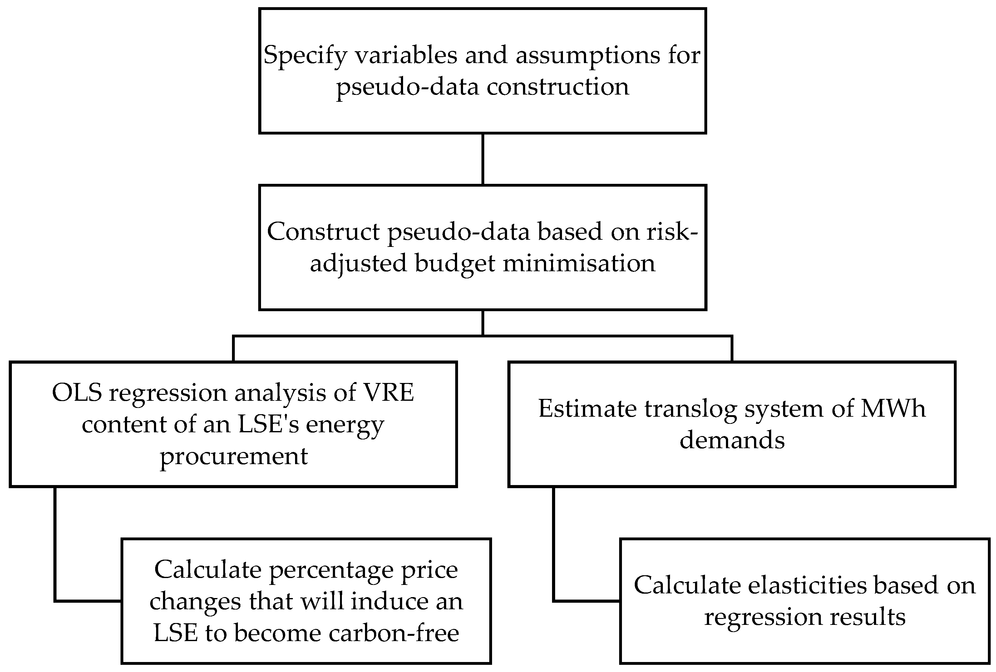
Our methodology entails the construction of a pseudo-dataset and two regression analyses to answer the five research questions set out in Section 1. These steps are summarised in Figure 1 and explained in detail in Section 2.1, Section 2.2, Section 2.3, Section 2.4 and Section 2.5 below.
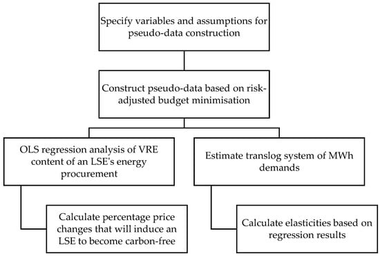
Figure 1.
Summary of the main steps of the methodology.
2.1. Assumptions and Scenarios for Pseudo-Data Construction
For clarity and concreteness, Table 1 lists the thirteen variables and their assumed values based on Texas’s market data. These variables are used to construct the pseudo-data used to specify the risk-adjusted budget minimisation problem: (1) Q = annual retail sales target of an LSE’s business plan; (2) Z = daytime share of Q; (3) α = daytime solar capacity factor; (4) ω = daytime wind capacity factor; (5) φ = nighttime wind capacity factor; (6) F1 = solar energy price; (7) F2 = wind energy price, assuming that a wind PPA typically has one energy price; (8) F3 = forward energy price; (9) μD = daytime spot energy price forecast; (10) σD = standard deviation of μD; (11) μN = nighttime spot energy price forecast; (12) σN = standard deviation of μN; and (13) ρ = correlation of μD and μN. Parenthetically, the high assumed values for α, ω, and φ aim to characterise solar plants and wind farms with battery storage, which helps realise a wholesale electricity market’s carbon-free supply.

Table 1.
Assumptions for constructing pseudo-data.
For mathematical tractability and expositional ease, we assume that variables (1) to (8) are non-stochastic but can have wide ranges of differing values. Variables (9) to (13) aim to characterise spot energy price forecasts by TOD. As each variable has three assumed values, a full factorial design yields 313 = 1,594,323 possible scenarios for solving an LSE’s risk-adjusted budget minimisation problem.
2.2. Risk-Adjusted Budget Minimisation
To meet its annual retail sales target, an LSE’s total energy procurement plan is Q = Q1 + Q2 + Q3 + Q4 + Q5, where Qj is the MWh amount of energy type j = 1 for solar, 2 for wind, 3 for forward, 4 for daytime spot, and 5 for nighttime spot. Generalising the formulation of [6], this section shows how Q1 to Q5 may come from risk-adjusted budget minimisation by an LSE.
We begin by recognising that an LSE procures solar and wind PPAs to serve retail pricing plans with VRE contents of up to 100%. Procuring K1 MW of solar capacity results in Q1 = H α K1 MWh of solar energy at a fixed energy price of $F1/MWh, where H = 12 daytime hours per day × number of days per year. Analogously, procuring K2 MW of wind capacity results in Q2 = H (ω + φ) K2 MWh of wind energy at a fixed energy price of $F2/MWh, as H is also the number of nighttime hours per year. Hence, the amounts of daytime and nighttime wind energy procured are [ω/(ω + φ)] Q2 and [φ/(ω + φ)] Q2.
The VRE content of Q is β = (Q1 + Q2)/Q = H [α K1 + (ω + φ) K2)]/Q. Let K = K1+ K2 so that ϕ = K1/K is the solar capacity share and (1 − ϕ)/K is the wind capacity share. As a result, an LSE’s VRE content is β = H [ϕ α + (1 − ϕ) (ω + φ)] K/Q, implying K = β Q ÷ H [ϕ α + (1 − ϕ) (ω + φ)].
The per MWh cost of VRE procurement is C1 = γ F1 + (1 − γ) F2, where γ is the solar energy share = Q1/(Q1 + Q2) = ϕ α/[ϕ α + (1 − ϕ) (ω + φ)] and (1 − γ) is the wind energy share = Q2/(Q1 + Q2) = (1 − ϕ) (ω + φ)/[ϕ α + (1 − ϕ) (ω + φ)]. Both C1 and γ are non-stochastic because ϕ, α, ω, φ, F1, and F2 are non-stochastic.
To meet the annual sales target, an LSE also procures a block of forward energy that equals Q3 MWh at a fixed energy price of $F3/MWh. The size of Q3 is the number of hours per year times the MW size of a signed forward contract for firm power delivery at the flat 100% rate. The amounts of daytime and nighttime forward energy are Q3/2 because of the equal number of daytime and nighttime hours per year.
The residually determined procurement of daytime spot energy is as follows:
which is bought at the daytime spot energy price of $PD/MWh. Analogously, the residually determined procurement of nighttime spot energy is as follows:
which is bought at the nighttime spot energy price of $PN/MWh. An LSE’s annual sales target is fully met because Q4 + Q5 = Q − Q1 − Q2 − Q3.
Q4 = Z Q − Q1 − [ω/(ω + φ)] Q2 − Q3/2,
Q5 = (1 − Z) Q − [φ/(ω + φ)] Q2 − Q3/2,
The per MWh cost of non-VRE procurement is C2 = λ F3 + (1 − λ) [ψ PD + (1 − ψ) PN], where λ = Q3/(Q3 + Q4 + Q5) denotes the forward energy share of non-VRE purchases and ψ = Q4/(Q4 + Q5) denotes the daytime share of spot energy purchases. As Q4 and Q5 are residually determined, ψ is not a choice variable in optimal procurement planning.
The forecast of C2 is μ2 = λ F3 + (1 − λ) [ψ μD + (1 − ψ) μN]. The variance of μ2 is σ22 = (1 − λ)2 [ψ2 σD2 + 2 ψ (1 − ψ) ρ σD σN + (1 − ψ)2 σN2]. As λ → 1, σ22 → 0, implying that an LSE can buy more forward energy to reduce its exposure to spot energy price variance.
The cost forecast for Q is θ = [β C1 + (1 − β) μ2] Q. Since ∂lnθ/∂lnQ = 1 for a given energy mix, it justifies the translog cost function’s specification shown in Appendix A under constant returns to scale. It also implies that a 1% increase in Q causes Qj to rise by 1%. Finally, the variance of θ is σθ2 = (1 − β)2 σ22 Q2. As β → 1, σθ2 → 0, implying that an LSE can procure more VRE to reduce σθ2. When β = 1, an LSE is carbon-free.
Following the value-at-risk concept [25], an LSE’s risk-adjusted budget is B = θ + 1.65 σθ so that the total procurement cost would not exceed B with a 0.95 probability under the assumption that θ is normally distributed per the central limit theorem. We assume that an LSE is financially prudent, implying that it aims to minimise B by choosing β, ϕ, and λ. This assumption reflects an LSE’s desire for financial solvency while bypassing the nuances of risk aversion elucidated in [31].
As each choice variable’s possible values are 0.0, 0.01, …, 0.99, 1.0, there are 1013 = 1,030,301 combinations of β, ϕ, and λ. Rather than using nonlinear programming [24], we adopt a simple grid search to find β*, ϕ*, and λ* that minimises B for one of the possible scenarios. This grid search comprises the following four steps:
- (1)
- Calculate the B values associated with the 1,030,301 combinations of β, ϕ, and λ for S1 that denote the first possible scenario.
- (2)
- Find the interior solutions for β*, ϕ*, and λ* for S1. To avoid the problem of empirically implausible elasticity estimates, the final sample only contains solutions with energy cost shares ≥ 0.05. These interior solutions realistically reflect that ~50% of Texas’s total installed generation capacity is solar and wind. Due to the need for revenue stability that aids the project financing of VRE developers, a majority of Texas’s total VRE capacity is sold via solar and wind PPAs to LSEs that offer retail pricing plans differentiated by VRE content (https://www.powertochoose.org). Further, unlike power traders, LSEs in Texas do not procure surplus VRE and forward energy on an annual basis for profitable resale in the wholesale spot energy market.
- (3)
- Use the results from Step (2) to calculate K* = optimal VRE capacity = β*Q ÷ H [ϕ∗ α + (1 − ϕ∗) (ω + φ)]; K1* = ϕ* K* = optimal solar capacity; K2* = (1 − ϕ*) K* = optimal wind capacity; Q1* = solar energy demand = H α ϕ* K*; Q2* = wind energy demand = H (ω + φ) (1 − ϕ*) K*; Q3*= forward energy demand = λ* (Q − Q1* − Q2*) = λ* (1 − β*) Q; Q4* = daytime spot energy demand = Z Q − Q1* − [ω/(ω + φ)] Q2* − Q3*/2; Q5* = nighttime spot energy demand = (1 − Z) Q − [φ/(ω + φ)] Q2* − Q3*/2; and β* = (Q1* + Q2*)/Q = optimal VRE content of Q. The resulting K*, K1*, K2*, Q1* to Q5*, and β* constitute the first observation for an LSE’s MWh demands.
- (4)
- Repeat Steps (1) to (3) to obtain K*, K1*, K2*, Q1* to Q5*, and β* for the remaining scenario Sn, where n = 2, …, N. As shown in Table 2, N = 1,062,822, which is lower than 1,594,323, the total number of possible scenarios. This discrepancy arises because some scenarios lack the necessary interior solutions.
Table 2.
Descriptive statistics of the pseudo-data used to obtain the empirics reported in Table 3, Table 4, Table 5 and Table 6; number of observations = 1,062,882.
| Panel A: Interior solutions for risk-adjusted budget minimisation | |||||
| Variable | Mean | Median | Standard Deviation | Minimum | Maximum |
| K1* (MW) | 290.20 | 55.71 | 494.13 | 1.17 | 2386.61 |
| K2* (MW) | 189.59 | 33.85 | 361.29 | 0.60 | 1990.33 |
| K1*/K2* | 8.44 | 2.33 | 12.24 | 0.03 | 99.00 |
| Q1* (MWh) | 564,322 | 105,869 | 886,528 | 3532 | 3,150,714 |
| Q2* (MWh) | 696,092 | 129,709 | 1,258,470 | 3389 | 4,578,648 |
| Q3* (MWh) | 561,555 | 126,592 | 1,142,985 | 3776 | 4,164,160 |
| Q4* (MWh) | 313,197 | 104,580 | 630,082 | 3483 | 3,143,878 |
| Q5* (MWh) | 544,834 | 126,039 | 799,643 | 5146 | 2,757,560 |
| β* | 0.47 | 0.50 | 0.29 | 0.05 | 0.91 |
| Panel B: Assumptions underlying the interior solutions shown in Panel A | |||||
| Variable | Mean | Median | Standard Deviation | Minimum | Maximum |
| Q (GWh) | 2680 | 2680 | 2520 | 160 | 5200 |
| Z | 0.55 | 0.55 | 0.08 | 0.45 | 0.65 |
| α | 0.50 | 0.50 | 0.16 | 0.30 | 0.70 |
| ω | 0.40 | 0.40 | 0.16 | 0.20 | 0.60 |
| ϕ | 0.50 | 0.50 | 0.16 | 0.30 | 0.70 |
| F1 ($/MWh) | 40 | 40 | 12.2 | 25 | 55 |
| F2 ($/MWh) | 40 | 40 | 12.2 | 25 | 55 |
| F3 ($/MWh) | 40 | 40 | 8.2 | 30 | 50 |
| μD ($/MWh) | 40 | 40 | 12.2 | 25 | 55 |
| σD ($/MWh) | 7.50 | 7.50 | 1.22 | 6.00 | 9.00 |
| μN ($/MWh) | 30 | 30 | 8.16 | 20 | 40 |
| σN ($/MWh) | 5.00 | 5.00 | 0.82 | 4.00 | 6.00 |
| ρ | 0.80 | 0.80 | 0.08 | 0.70 | 0.90 |
Note: The minimum value of Q is different from the low value of Q in Table 1 because of excluding implausible observations with Wj < 0.05.
2.3. What Induces an LSE to Become Carbon-Free?
This question is related to the market economics of a carbon-free electric grid [14]. We answer the question by estimating OLS regression, for which the regressand is β* and the regressors are the thirteen variables listed in Table 1.
Based on the data portrayed in Table 2, the OLS regression results in Table 3 yield two price-based answers. The first answer is the decline in VRE prices. Suppose η1 = ∂β*/∂lnF1 < 0 and η2 = ∂β*/∂lnF2 < 0. Absent of changes in the other regressors, Δβ* = η1 ΔlnF1 + η2 ΔlnF2 = (η1 + η2) ζ, where ζ ≡ equals the percentage change in VRE prices = ΔlnF1 = ΔlnF2. Let β0 < 1 denote Q’s existing VRE content so that an LSE’s carbon-free condition is Δβ* = (1 − β0) > 0. Hence, an LSE is induced to become carbon-free when ζ = (1 − β0)/(η1 + η2) < 0, which may occur if the trend in declining solar and wind energy prices continues [10,11].
The second answer is the increase in non-VRE prices. Suppose η3 = ∂β*/∂lnF3 > 0, ηD = ∂β*/∂lnμD > 0 and ηN = ∂β*/∂lnμN > 0. An LSE is induced to become carbon-free when ν = (1 − β0)/(η3 + ηD + ηN) > 0, which is the equal percentage increase in non-VRE prices that may occur due to rising wholesale natural gas prices and growing system electricity demands.
Table 3.
OLS regression analysis of β*; number of observations = 1,062,882 based on Table 2.
Table 3.
OLS regression analysis of β*; number of observations = 1,062,882 based on Table 2.
| Panel A: Regression results | |||||||||
| Variable (Coefficient of Primary Interest) | Estimate | Standard Error | p-Value | ||||||
| Regressand’s mean | 0.4723 | ||||||||
| Adjusted R2 | 0.6687 | ||||||||
| RMSE | 0.1681 | ||||||||
| Intercept | 1.6436 | 0.0057 | <0.001 | ||||||
| lnZ | 0.2608 | 0.0011 | <0.001 | ||||||
| lnα | 0.0033 | 0.0005 | <0.001 | ||||||
| lnω | 0.0049 | 0.0004 | <0.001 | ||||||
| lnϕ | 0.0068 | 0.0005 | <0.001 | ||||||
| lnρ | 0.0035 | 0.0016 | 0.029 | ||||||
| lnQ | −0.0012 | 0.0001 | <0.001 | ||||||
| lnF1 (η1) | −0.2520 | 0.0005 | <0.001 | ||||||
| lnF2 (η2) | −0.6071 | 0.0004 | <0.001 | ||||||
| lnF3 (η3) | 0.3659 | 0.0008 | <0.001 | ||||||
| lnμD (ηD) | 0.2089 | 0.0011 | <0.001 | ||||||
| lnσD | 0.0071 | 0.0010 | <0.001 | ||||||
| lnμN (ηN) | 0.0193 | 0.0011 | <0.001 | ||||||
| lnσN | 0.0064 | 0.0010 | <0.001 | ||||||
| Panel B: Estimated percentage price changes that would induce an LSE to become carbon-free | |||||||||
| Percentage Price Change | β0 = Existing VRE Content | ||||||||
| 0.1 | 0.2 | 0.3 | 0.4 | 0.5 | 0.6 | 0.7 | 0.8 | 0.9 | |
| VRE: ζ = (1 − β0)/(η1 + η2) | −104.8% | −93.1% | −81.5% | −69.8% | −58.2% | −46.6% | −34.9% | −23.3% | −11.6% |
| Non-VRE: ν = (1 − β0)/(η3 + ηD + ηN) | 151.5% | 134.7% | 117.8% | 101.0% | 84.2% | 67.3% | 50.5% | 33.7% | 16.8% |
2.4. Translog Specification of a System of MWh Demands
Following [28], we adopt a translog specification that is less restrictive than the constant elasticity of substitution specifications for a two-input demand system [32] used in [6] for our analysis of five MWh demands. Our regression setup begins with VD = σD/μD and VN = σN/μN, which are coefficients of variation unaffected by a proportional change in daytime and nighttime spot energy prices. However, VD and VN can be magnified by mean-preserving increases in σD and σN. As a result, VD and VN help detect the demand effects of absent σD and σP changes in μD and μN. Finally, ρ enters an LSE’s MWh demands because of B*’s dependence on ρ, which increases non-VRE’s procurement cost variance σ22.
Let Wj ≥ 0.05 denote the discernible cost share of Qj* (i.e., W1 = F1 Q1*/θ* > 0.05, W2 = F2 Q2*/θ* > 0.05, etc.) based on the data portrayed in Table 2. Had the observations with Wj < 0.05 been included, they would have led to anomalous coefficient estimates and empirically implausible price elasticity estimates [32]. As the number of observations exceeds one million, the empirics reported in Table 4 and Table 5 are deemed credible.
Table 4.
Iterated SUR results; number of observations = 1,062,882 based on Table 2.
Table 4.
Iterated SUR results; number of observations = 1,062,882 based on Table 2.
| Variable | Equation (1): Regressand = W1 | Equation (2): Regressand = W2 | Equation (3): Regressand = W3 | Equation (4): Regressand = W4 | ||||
|---|---|---|---|---|---|---|---|---|
| Estimate | Standard Error | Estimate | Standard Error | Estimate | Standard Error | Estimate | Standard Error | |
| Sample mean of Wj | 0.2281 | 0.2528 | 0.2118 | 0.121 | ||||
| Adjusted R2 | 0.5140 | 0.6348 | 0.5291 | 0.4227 | ||||
| RMSE | 0.1338 | 0.1586 | 0.1750 | 0.1060 | ||||
| Intercept | 0.3543 | 0.0013 | 0.4615 | 0.0016 | 0.3348 | 0.0018 | 0.1026 | 0.0012 |
| lnF1 | −0.2296 | 0.0004 | 0.0825 | 0.0003 | 0.1496 | 0.0004 | 0.1700 | 0.0003 |
| lnF2 | 0.0825 | 0.0003 | −0.5963 | 0.0005 | 0.2685 | 0.0004 | 0.0467 | 0.0003 |
| lnF3 | 0.1496 | 0.0004 | 0.2685 | 0.0004 | −0.6997 | 0.0007 | 0.0846 | 0.0004 |
| lnμD | 0.1700 | 0.0003 | 0.0467 | 0.0003 | 0.0846 | 0.0004 | −0.1866 | 0.0004 |
| lnμN | −0.1726 | 0.0002 | 0.1986 | 0.0003 | 0.1971 | 0.0004 | −0.1147 | 0.0003 |
| lnZ | 0.4439 | 0.0009 | −0.1724 | 0.0010 | −0.1145 | 0.0011 | 0.2025 | 0.0007 |
| lnVD | −0.0313 | 0.0004 | 0.0491 | 0.0005 | 0.0394 | 0.0006 | −0.0157 | 0.0004 |
| lnVN | −0.0185 | 0.0004 | 0.0931 | 0.0005 | 0.0335 | 0.0006 | −0.0393 | 0.0004 |
| lnρ | 0.0008 | 0.0013 | 0.0028 | 0.0015 | 0.0079 | 0.0017 | −0.0065 | 0.0010 |
| lnα | 0.0060 | 0.0004 | −0.0009 | 0.0004 | −0.0019 | 0.0005 | −0.0037 | 0.0003 |
| lnω | −0.0506 | 0.0003 | 0.0498 | 0.0003 | −0.0107 | 0.0004 | −0.0263 | 0.0002 |
| lnϕ | 0.0508 | 0.0004 | −0.0382 | 0.0004 | 0.0064 | 0.0005 | 0.0246 | 0.0003 |
Note: Except those for lnρ in Equations (1) and (2) and lnα in Equation (2), all coefficient estimates are highly significant with p-values < 0.001.
Table 5.
Estimated price responsiveness based on the median values of {Ejk}.
Table 5.
Estimated price responsiveness based on the median values of {Ejk}.
| MWh Demand | Elasticities of Qj* with Respect to the Variables Listed Below | ||||
|---|---|---|---|---|---|
| F1 | F2 | F3 | μD | μN | |
| Q1* | −2.63 | 1.57 | 2.82 | 3.42 | −1.50 |
| Q2* | 0.95 | −10.52 | 4.90 | 0.97 | 2.24 |
| Q3* | 1.54 | 4.42 | −13.10 | 1.69 | 2.18 |
| Q4* | 1.45 | 0.81 | 1.57 | −4.49 | −0.98 |
| Q5* | −1.22 | 3.47 | 3.66 | −1.93 | −1.87 |
Based on the translog cost function’s specification in Appendix A, Equations (1)–(5) stated below are seemingly unrelated regressions (SURs) with additive random errors of ε1 to ε5 that are contemporaneously correlated [27]:
W1 = a1 + b11 lnF1 + b12 lnF2 + b13 lnF3 + b14 lnμD + b15 lnμN + b1Z lnZ + b1VD lnVD + b1VN lnVN + b1ρ lnρ + b1α lnα + b1ω lnω + b1φ lnφ + ε1.
W2 = a2 + b12 lnF1 + b22 lnF2 + b23 lnF3 + b24 lnμD + b25 lnμN + b2Z lnZ + b2VD lnVD + b2VN lnVN + b2ρ lnρ + b2α lnα + b2ω lnω + b2φ lnφ + ε2.
W3 = a3 + b13 lnF1 + b23 lnF2 + b33 lnF3 + b34 lnμD + b35 lnμN + b3Z lnZ + b3VD lnVD + b3VN lnVN + b3ρ lnρ + b3α lnα + b3ω lnω + b3φ lnφ + ε3.
W4 = a4 + b14 lnF1 + b24 lnF2 + b34 lnF3 + b44 lnμD + b45 lnμN + b4Z lnZ + b4VD lnVD + b4VN lnVN + b4ρ lnρ + b4α lnα + b4ω lnω + b4φ lnφ + ε4.
W5 = a5 + b15 lnF1 + b25 lnF2 + b35 lnF3 + b45 lnμD + b55 lnμN + b5Z lnZ + b5VD lnVD + b5VN lnVN + b5ρ lnρ + b5α lnα + b5ω lnω + b5φ lnφ + ε5.
Since ∑j Wj = 1, Equations (1)–(5) embody the following coefficient restrictions: ∑j aj = 1; bjk = bkj; ∑k bjk = 0; ∑j bjk = 0; and ∑j bjX = 0 for lnX = lnZ, lnVD, lnVN, lnρ, lnα, lnω, or lnφ [28]. Further, lnQ does not appear in Equations (1)–(5) because of the procurement cost function’s property of constant returns to scale. As a joint estimation of Equations (1)–(5) is infeasible due to ∑j Wj = 1, we use the iterated SUR technique to estimate Equations (1)–(4). We then apply the coefficient restrictions to find Equation (5)’s coefficient estimates for calculating the elasticities stated in the next section. To empirically verify constant returns to scale, we repeat the SUR estimation by including lnQ as regressors in Equations (1)–(5), finding that the coefficient estimates for lnQ are for all practical purposes equal to zero.
2.5. Elasticities
The solar MWh demand’s own-price elasticity is E11 = ∂lnQ1*/∂lnF1 = (b11/W1) + W1 − 1, and the first cross-price elasticity is E12 = ∂lnQ1*/∂lnF2 = (b12/W1) + W2 [27]. Omitted for brevity, the remaining price elasticities can be found analogously.
We use EjX = ∂lnQj*/∂lnX to measure the percentage change in Qj* due to a one percent change in X, where X = Z, VD, VN, ρ, α, ω, or φ. Appendix A shows EjX = (bjX/Wj) + b1X lnF1 + b2X lnF2 + b3X lnF3 + b4X lnμD + b5X lnμN.
Since the elasticity formulae are nonlinear, we first calculate Ejk and EjX for each observation in our estimation sample. Some observation-specific elasticity estimates tend to have large sizes when Wj is close to 0.05. Hence, we adopt the median values of Ejk and EjX to gauge Qj*’s responsiveness because the median values are less influenced than the mean values by the extreme observation-specific elasticity estimates.
3. Empirics
Table 2 provides descriptive statistics of the large sample of pseudo-data used to obtain the empirics reported in Table 3, Table 4, Table 5 and Table 6. It shows that these data exhibit large variations, thus enabling a meaningful statistical analysis of an LSE’s demand for various sources of energy generation.
Table 6.
Other elasticity estimates based on the median values of {EjX}.
Table 6.
Other elasticity estimates based on the median values of {EjX}.
| MWh Demand | Elasticities of Qj* with Respect to the Variables Listed Below | ||||||
|---|---|---|---|---|---|---|---|
| Z | VD | VN | ρ | α | ω | ϕ | |
| Q1* | 3.56 | −0.23 | −0.13 | 0.01 | 0.05 | −0.40 | 0.41 |
| Q2* | −2.68 | 0.82 | 1.54 | 0.05 | −0.01 | 0.80 | −0.61 |
| Q3* | −1.84 | 0.70 | 0.60 | 0.14 | −0.03 | −0.19 | 0.11 |
| Q4* | 3.83 | −0.28 | −0.71 | −0.12 | −0.07 | −0.50 | 0.46 |
| Q5* | −3.02 | −0.37 | −0.61 | −0.05 | 0.01 | 0.32 | −0.37 |
Answering the second research question is Panel A of Table 2, which reports that the ratio of mean K1* to mean K2* is (290.2/189.6) = 1.53. When based on the median values of K1* and K2*, the (K1*/K2*) ratio becomes (55.71/33.85) = 1.65. Finally, the median of the observation-specific (K1*/K2*) ratios is 2.33. Hence, an LSE tends to procure far more solar capacity than wind capacity, thus corroborating the solar and wind capacity additions noted in Section 1. This finding is important because it lends support to the real-world relevance and empirical validity of our pseudo-data construction.
Answering the third research question is Panel A of Table 3, which reports the results of the OLS regression analysis of an LSE’s optimal VRE content. The adjusted R2 of 0.67 indicates a reasonable goodness of fit for a cross-sectional sample of over one million observations. Further, all coefficient estimates are significant, with p-values well below 0.05.
Suppose an LSE’s existing VRE content is ~27% based on the share of Texas’s total electricity generation in 2023 from VRE sources. Panel B of Table 3 shows that inducing this LSE to become carbon-free would require the VRE energy prices to decline by over 81.5% or the non-VRE energy prices to increase by over 117.8%. However, if the existing VRE content is already at 90%, the required VRE price decline is 11.6%, and the required non-VRE price increase is 16.8%. As a result, LSEs with relatively high existing VRE content are likely to become carbon-free in response to moderate changes in VRE and non-VRE prices, unlike those with relatively low existing VRE content.
Answering the first research question is Table 4, which reports adjusted R2 values of 0.42 to 0.63, indicating the reasonable goodness-of-fit of our parsimoniously specified SUR system. With three exceptions, all coefficient estimates are statistically significant with p-values ≤ 0.01. Hence, we use Table 4’s regression results to calculate the elasticity estimates presented in Table 5 and Table 6.
Answering the fourth research question is Table 5, which shows that an LSE’s MWh demands are price-elastic, with own-price elasticity estimates ranging from −1.87 for nighttime spot MWh demand to −13.1 for forward MWh demand. These large own-price elasticity estimates mirror an LSE’s ex ante procurement choices under multiple energy supply sources. The cross-price elasticity estimates indicate that except for nighttime wind energy, all energy types are substitutes in an LSE’s procurement plan.
Answering the fifth research question is Table 6, which reports the other elasticity estimates. Emerging from Table 6 are the following remarks:
- The daytime share of an LSE’s annual sales target matters. Specifically, a 1% increase in Z tends to raise Q1* and Q4* by 3.6% to 3.8% and reduce Q2*, Q3*, and Q5* by 1.8% to 3.0%.
- The coefficients of variation in the energy price forecasts by TOD matter. A 1% increase in VD tends to reduce Q1* by 0.23% but increase Q2* by 0.82%. A 1% increase in VN tends to reduce Q1* by 0.13% but increase Q2* by 1.54%. Hence, stabilizing spot energy prices by TOD due to an increase in ERCOT’s operating and planning reserves tends to have relatively small effects on solar and wind MWh demands.
- Changes in solar and wind capacity factors have mixed effects on solar and wind MWh demands. To wit, a 1% increase in α tends to increase solar MWh demand by 0.05% and reduce wind MWh demand by 0.01%. Hence, marginally improving VRE generation’s output performance is unlikely to materially increase solar and wind MWh demands. This makes sense because of an LSE’s focus on VRE delivery, implying that the LSE’s procurement of VRE capacities has already accounted for the delivery effects of VRE capacity factor improvements.
4. Conclusions and Policy Implications
Our conclusions are as follows. First, the MWh demands of an LSE in the presence of multiple supply sources and wholesale electricity price uncertainty have not been explored in the literature of non-residential electricity demand estimation. Second, these MWh demands are the result of an LSE’s procurement planning based on risk-adjusted budget minimisation. Third, the pseudo-data approach overcomes the frequent lack of disaggregate data for PPA transactions and spot energy purchases. Fourth, using a large pseudo-data sample of over one million observations, we find the estimated changes in VRE and non-VRE prices that would induce an LSE to become carbon-free. Fifth, we use the same sample to obtain price elasticity estimates that indicate that an LSE’s MWh demands are price-elastic and responsive to changes in the drivers that are unrelated to energy price levels. Finally, the daytime share of an LSE’s total retail sales target matters in solar and wind MWh demands.
The policy implications of the last three conclusions are as follows. First, an LSE with relatively high existing VRE content may become carbon-free sans further government intervention (e.g., a carbon tax on CO2-emitting generation or additional tax credits for VRE investment and production). This is because Table 3 shows that an LSE’s VRE content tends to rise in response to (a) declining solar and wind energy prices due to VRE’s falling per MWh costs [10,11] or (b) rising forward and spot energy prices due to increases in natural gas price and electricity demand.
Second, the price management of VRE demands is effective. Suppose ERCOT imposes a $1 per MWh charge on VRE generators to recover the incremental cost for operating reserves due to rising VRE generation [30]. This hypothetical charge likely raises the energy prices of solar and wind PPAs by about 2% based on the US average energy price of $50/MWh for VRE in the first quarter of 2023, as VRE developers tend to fully pass the charge in their supply offers in response to an LSE’s procurement auction [22]. Using the own- and cross-price elasticity estimates in Table 5, we find that the hypothetical $1/MWh charge is expected to alter solar MWh demands by −2.1% [= 2% (E11 + E12) = 2% (−2.63 + 1.57)] and wind MWh demands by −19.1% [=2% (E21 + E22) = 2% (0.95–10.52)]. Hence, the charge’s implementation has a greater effect on an LSE’s demand for wind than its demand for solar generation.
Finally, retail time of use (TOU) pricing matters in an LSE’s solar and wind MWh demands. Based on the E1Z and E2Z estimates in Table 6, a 1% decrease in the daytime share of an LSE’s annual sales target tends to reduce solar MWh demands by 3.56% and increase wind MWh demands by 2.68%, chiefly because an LSE has lower daytime but higher nighttime retail sales under TOU pricing. This also means less solar generation but more wind generation that at least historically tended to pose challenges to maintaining real-time system load-resource balance in ERCOT [33].
In closing, the preceding implications present policy and regulatory challenges in an electric grid’s pathway to deep decarbonisation, as implementing piecemeal policy measures can have conflicting outcomes. A good case in point is the $1 increase in the per MWh charge for operating reserves that reduces wind MWh demands and retail TOU pricing that increases wind MWh demands. As a result, integrated resource planning under wholesale electricity market competition [34] is essential for solving an electric grid’s twin goals of deep decarbonisation [13] and providing electric service at stable and economically efficient prices.
There are a few caveats in this paper that can lead to fruitful future research. First, the translog function is only one of the five parametric specifications commonly used in non-residential electricity demand estimation [26]. Hence, a fruitful area of research is to test if the estimated price responsiveness of an LSE’s MWh demands is sensitive to the choice of a parametric specification. Second, risk-adjusted budget minimisation is not the only approach to generate the pseudo-data for an LSE’s MWh demands. Other approaches are available, including efficient frontiers [21], multi-period VaR-constrained portfolio optimization [35], and option theory [36]. Hence, applying the other approaches to construct pseudo-data is another fruitful area of future research. Finally, our estimation of an LSE’s MWh demands does not address the many thorny issues that hinder an electric grid’s ability to provide reliable service at stable prices. A partial list of these issues includes inadequate investment incentives for natural-gas-fired generation, wholesale energy trading inefficiency, interregional transmission constraints, possible market power abuse by some independent power producers, and inefficient retail pricing under wholesale market competition. Hence, far more research is necessary to resolve these issues, well beyond what this paper intends to accomplish.
Author Contributions
Conceptualization, C.-K.W.; data curation, K.H.C.; formal analysis, K.H.C. and H.S.Q.; methodology, C.-K.W.; writing—original draft, K.H.C. and H.S.Q.; writing—review and editing, J.W.Z. and R.L. All authors have read and agreed to the published version of the manuscript.
Funding
This study is funded by the Ford Foundation’s grants (#134371 and #139746) and the Research Matching Grant Scheme of the Research Grant Council of the Hong Kong Special Administrative Region and the National Natural Science Foundation of China (#72473103).
Data Availability Statement
The data used in this study are available from the corresponding author upon request.
Conflicts of Interest
The authors declare no conflict of interest.
Abbreviations
ERCOT, Electric Reliability Council of Texas; LSE, load serving entity; OLS, ordinary least squares; PPA, power purchase agreement; SUR, seemingly unrelated regression; TOD, time of day; UN, United Nations; US, United States; VRE, variable renewable energy.
Appendix A. Formula for Calculating EjX
Let TC = total cost for producing a given level of output denoted by Q. Under constant returns to scale, TC = C(P, Y) Q, where C(P, Y) = average cost function, P = vector of input prices, and Y = vector of non-price factors [27]. Invoking Shephard’s Lemma [37], we find that the vector of input demands is ∂TC/∂P = [∂C(P, Y)/∂P] Q, implying that a 1% increase in Q would raise all input demands by 1%. Further, estimating the price responsiveness of input demands can be based on the following translog specification of C(P, Y):
where C = cost per unit of output, Pj = input price j for j = 1 to J, and Ym = non-price factor m for m = 1 to M. Based on Shephard’s Lemma, the cost share of input usage Qj per unit of output is ∂lnC/∂lnPj = Wj = Pj Qj/C = αj + ∑k βjk lnPk + ∑m δjm lnYm so that ∂Wj/∂lnYm = δjm. Further, lnWj = lnPj + lnQj − lnC, implying ∂lnWj/∂lnYm = ∂lnQj/∂lnYm − ∑j δjm lnPj because ∂lnC/∂lnYm = ∑j δjm lnPj.
lnC = ∑j αj lnPj + ½ ∑j ∑k βjk lnPj lnPk + ∑j ∑m δjm lnPj lnYm,
Since ∂lnWj/∂lnYm = (∂lnWj/∂Wj ) (∂Wj/∂lnYm) = δjm/Wj, we obtain
∂lnQj/∂lnYm = δjm/Wj + ∑j δjm lnPj.
When based on the notations used in Section 2.4, Equation (A2) leads to the formula stated in Section 2.5:
∂lnQj/∂lnX = bjX/Wj + b1X lnF1 + b2X lnF2 + b3X lnF3 + b4X lnμD + b5X lnμN.
References
- Mahone, A.; Subin, Z.; Orans, R.; Miller, M.; Regan, L.; Calviou, M.; Saenz, M.; Bacalao, N. On the path of decarbonization. IEEE Power Energy Mag. 2018, 16, 58–68. [Google Scholar] [CrossRef]
- Poudyal, R.; Loskot, P.; Nepal, R.; Parajuli, R.; Khadka, S.K. Mitigating the current energy crisis in Nepal with renewable energy sources. Renew. Sustain. Energy Rev. 2019, 116, 109388. [Google Scholar] [CrossRef]
- Simshauser, P. Merchant renewables and the valuation of peaking plant in energy-only markets. Energy Econ. 2020, 91, 104888. [Google Scholar] [CrossRef]
- Peña, J.I.; Rodríguez, R.; Mayoral, S. Cannibalization, depredation, and market remuneration of power plants. Energy Policy 2022, 167, 113086. [Google Scholar] [CrossRef]
- Li, Y.; Tang, X.; Liu, M.; Chen, G. The benefits and burdens of wind power systems in reaching China’s renewable energy goals: Implications from resource and environment assessment. J. Clean. Prod. 2024, 481, 144134. [Google Scholar] [CrossRef]
- Woo, C.K.; Cao, K.H.; Qi, H.S.; Zarnikau, J.; Li, R. Price responsiveness of solar and wind capacity demands. J. Clean. Prod. 2024, 462, 142705. [Google Scholar] [CrossRef]
- Energy Institute. Statistical Review of World Energy 2024. Available online: https://www.energyinst.org/statistical-review (accessed on 20 January 2025).
- Kapica, J.; Canales, F.A.; Jurasz, J. Global atlas of solar and wind resources temporal complementarity. Energy Convers. Manag. 2021, 246, 114692. [Google Scholar] [CrossRef]
- Alagappan, L.; Orans, R.; Woo, C.K. What drives renewable energy development? Energy Policy 2011, 39, 5099–5104. [Google Scholar] [CrossRef]
- Bolinger, M.; Seel, J.; Warner, C.; Robson, D. Utility-Scale Solar, 2021 Edition: Empirical Trends in Deployment, Technology, Cost, Performance, PPA Pricing, and Value in the United States. 2021. Lawrence Berkeley National Laboratory. Available online: https://escholarship.org/content/qt080872q5/qt080872q5.pdf (accessed on 9 December 2024).
- Wiser, R.; Bolinger, M.; Hoen, B.; Millstein, D.; Rand, J.; Barbose, G.; Darghouth, N.; Gorman, W.; Jeong, S.; Mills, A.; et al. Land-Based Wind Market Report: 2021 Edition. 2021. Lawrence Berkeley National Laboratory. Available online: https://escholarship.org/content/qt4sb6r5mz/qt4sb6r5mz.pdf (accessed on 9 December 2024).
- Carvallo, J.P.; Murphy, S.P.; Sanstad, A.; Larsen, P.H. The use of wholesale market purchases by U.S. electric utilities. Energy Strategy Rev. 2020, 30, 100508. [Google Scholar] [CrossRef]
- Williams, J.H.; DeBenedictis, A.; Ghanadan, R.; Mahone, A.; Moore, J.; Morrow, W.R.; Price, S.; Torn, M.S. The technology path to deep greenhouse gas emissions cuts by 2050: The pivotal role of electricity. Science 2012, 6064, 53–59. [Google Scholar] [CrossRef] [PubMed]
- Milstein, I.; Asher, A.; Woo, C.K. Carbon-free electricity supply in a Cournot wholesale market: Israel. Energy J. 2024, 45, 69–89. [Google Scholar] [CrossRef]
- Davis, L.; Hausman, C.; Rose, N. Transmission impossible? Prospects for decarbonizing the US grid. J. Econ. Perspect. 2023, 37, 155–180. [Google Scholar] [CrossRef]
- Holttinen, H.; Groom, A.; Kennedy, E.; Woodfin, D.; Barroso, L.; Orths, A.; Ogimoto, K.; Wang, C.; Moreno, R.; Parks, K.; et al. Variable renewable energy integration: Status around the world. IEEE Power Energy Mag. 2021, 19, 86–96. [Google Scholar] [CrossRef]
- Public Utility Commission of Texas. Scope of Competition in Electric Markets in Texas: Report to the 86th Legislature. 2019. Available online: https://ftp.puc.texas.gov/public/puct-info/industry/electric/reports/scope/2019/2019scope_elec.pdf (accessed on 28 January 2025).
- Ela, E.; Billimoria, F.; Ragsdale, K.; Moorty, S.; O’Sullivan, J.; Gramlich, R.; Rothleder, M.; Rew, B.; Supponen, M.; Sotkiewicz, P. Future electricity markets: Designing for massive amounts of zero-variable-cost renewable resources. IEEE Power Energy Mag. 2021, 17, 58–66. [Google Scholar] [CrossRef]
- Roselund, C. Is the U.S. Solar Market Slipping towards Merchant? 2019. Available online: https://www.pv-magazine.com/2019/06/24/is-the-u-s-solar-market-slipping-towards-merchant/ (accessed on 9 December 2024).
- Gohdes, N.; Simshauser, P.; Wilson, C. Renewable entry costs, project finance and the role of revenue quality in Australia’s National Electricity Market. Energy Econ. 2022, 114, 106312. [Google Scholar] [CrossRef]
- Cao, K.H.; Qi, H.S.; Woo, C.K.; Zarnikau, J.; Li, R. Efficient frontiers for short-term sales of spot and forward wind energy in Texas. Energy J. 2024, 45, 37–60. [Google Scholar] [CrossRef]
- Qi, H.S.; Cao, K.H.; Woo, C.K.; Zarnikau, J.; Li, R. Revenue analysis of spot and forward solar energy sales in Texas. J. Energy Mark. 2024, 17, 1–38. [Google Scholar] [CrossRef]
- Wolak, F.A.; Kolstad, C.D. A model of homogeneous input demand under price uncertainty. Am. Econ. Rev. 1991, 81, 514–538. [Google Scholar]
- Woo, C.K.; Karimov, R.; Horowitz, I. Managing electricity procurement cost and risk by a local distribution company. Energy Policy 2004, 32, 635–645. [Google Scholar] [CrossRef]
- Jorion, P. Value at Risk; Irwin: Chicago, IL, USA, 1997. [Google Scholar]
- Li, R.; Woo, C.K. How price responsive is commercial electricity demand in the US? Electr. J. 2022, 35, 107066. [Google Scholar] [CrossRef]
- Greene, W.H. Econometric Analysis, 8th ed.; Pearson: New York, NY, USA, 2017. [Google Scholar]
- Griffin, J.M. Long-run production modeling with pseudo data: Electric power generation. Bell J. Econ. 1977, 8, 112–127. [Google Scholar] [CrossRef]
- Ming, Z.; Delgado, D.; Schlag, N.; Olson, A.; Wintermantel, N.; Dombrowky, A.; Amitava, R. Assessment of Market Reform Options to Enhance Reliability of the ERCOT System; Report Prepared by Energy and Environmental Economics, Inc. (E3) for the Public Utility Commission of Texas; Energy and Environmental Economics, Inc.: San Francisco, CA, USA, 2022. [Google Scholar]
- Sioshansi, F.P. Evolution of Global Electricity Markets: New Paradigms, New Challenges, New Approaches; Elsevier: Amsterdam, The Netherlands, 2013. [Google Scholar]
- Menezes, C.F.; Hanson, D.L. On the theory of risk aversion. Int. Econ. Rev. 1970, 11, 481–487. [Google Scholar] [CrossRef]
- Caves, D.W.; Christensen, L.R. Global properties of flexible functional forms. Am. Econ. Rev. 1980, 70, 422–432. [Google Scholar]
- Sioshansi, R.; Hurlbut, D. Market protocols in ERCOT and their effect on wind generation. Energy Policy 2010, 38, 3192–3197. [Google Scholar] [CrossRef]
- Wilkerson, J.; Larsen, P.; Barbose, G. Survey of Western U.S. electric utility resource plans. Energy Policy 2014, 66, 90–103. [Google Scholar] [CrossRef]
- Kleindorfer, P.R.; Li, L. Multi-period VaR-constrained portfolio optimization with applications to the electric power Sector. Energy J. 2005, 26, 1–26. [Google Scholar] [CrossRef]
- Haar, L.; Haar, L. An option analysis of the European Union renewable energy support mechanisms. Econ. Energy Environ. Policy 2017, 6, 131–148. [Google Scholar] [CrossRef]
- Varian, H.R. Microeconomic Analysis, 3rd ed.; Norton: New York, NY, USA, 1992. [Google Scholar]
Disclaimer/Publisher’s Note: The statements, opinions and data contained in all publications are solely those of the individual author(s) and contributor(s) and not of MDPI and/or the editor(s). MDPI and/or the editor(s) disclaim responsibility for any injury to people or property resulting from any ideas, methods, instructions or products referred to in the content. |
© 2025 by the authors. Licensee MDPI, Basel, Switzerland. This article is an open access article distributed under the terms and conditions of the Creative Commons Attribution (CC BY) license (https://creativecommons.org/licenses/by/4.0/).