Virtual Synchronous Generator Based on Hybrid Multi-Vector Model Predictive Control

Abstract

This paper proposes a hybrid multi-vector model predictive control (MPC) to reduce the harmonic content in the output current of a two-level virtual synchronous generator (VSG). Compared to traditional two-vector MPC, the proposed hybrid multi-vector MPC has twelve sets of voltage vectors, meaning that the number of iterative calculations required in each cycle is identical for both control methods. Compared to the three-vector MPC, the proposed method requires more iterative calculations per control period but achieves optimal harmonic content in the output current. In addition, different from the traditional MPC methods, this paper incorporates frequency variation weights into the cost function, which further reduces the harmonic content in the output current. Finally, the effectiveness of the proposed control strategy is validated through a simulation model built in MATLAB/Simulink.

1. Introduction

With the exhaustion of traditional fossil energy, distributed generation, especially comprising wind and solar energy sources, has gained substantial popularity owing to its minimal environmental impact and abundant renewable resources [1]. Distributed energy sources are typically integrated into the grid through power electronic converters. However, unlike synchronous generators, power electronic converters lack inertia and damping, which can result in insufficient system inertia and damping when distributed energy sources are extensively integrated into the grid. The system becomes less resilient to disturbances and is more susceptible to frequency collapse under severe disturbances [2,3]. To address this issue, the concept of virtual synchronous generator (VSG) control has been introduced, where power electronic converters emulate the inertia and damping, as well as the active frequency regulation and reactive voltage regulation capabilities of synchronous generators to support the grid [4,5,6,7].

VSG control typically employs a double-loop control strategy, which is straightforward to implement and easy to understand [8,9,10,11]. In [12,13,14,15], an adaptive control strategy was proposed. The output characteristics of the converter are optimized by adjusting the rotational inertia and damping in real time when the load is disturbed. In [16,17], the control delay was considered, and a distributed secondary control strategy was proposed to optimize the output characteristics of the inverter. However, these methods suffer from the same drawbacks, i.e., high control complexity and slow dynamic response, as the inner loop uses closed-loop control based on a proportional-integral controller. Model predictive control (MPC) has gained significant attention due to its rapid dynamic response and multi-objective optimization capabilities. The application of MPC in VSG can effectively address the issue of slow dynamic response in the existing double-loop control.

In [18], the mathematic model and frequency control strategy of VSGs were investigated through MPC. In [19,20], a single-vector MPC was proposed for a two-level converter. In this method, eight voltage vectors are used to control the output current. It is easy to implement; however, the high harmonic content of the output current necessitates additional filters to meet power quality requirements. To improve the quality of the VSG output current, references [21,22,23] proposed a two-vector MPC method based on virtual vectors. This method includes 12 sets of voltage vectors, leading to an overall improvement in the quality of the output current compared to the single-vector MPC method. In addition, a three-vector MPC was proposed in [24,25,26]. The three-vector MPC consists of six sets of voltage vectors, each containing three vectors, which is one vector more than the two-vector MPC. However, although the three-vector MPC expands the coverage of voltage vectors, the harmonic content of the output current using this method is not better than that of the two-vector MPC in all cases. A hybrid multi-vector MPC strategy for voltage source inverter was introduced in [27]. This method minimizes the harmonic content of the output current, but it requires 18 iterations of computation per switching cycle, demanding a controller with higher performance.

Therefore, to minimize current harmonic content without increasing the controller cost, a hybrid multi-vector MPC method is proposed in this paper. First, the cost functions of two-vector MPC and three-vector MPC are analyzed. By comparing the values of the cost functions of both methods, it is demonstrated that neither achieves global optimization of the harmonic content of the output current. Then, a hybrid multi-vector MPC strategy is proposed. In the proposed strategy, to avoid increasing the number of iterative computations per control cycle, new vector sets are introduced by analyzing the vector sets of the two-vector MPC and three-vector MPC. Compared to the two-vector MPC, this proposed strategy ensures that the voltage vector sets with the lowest current harmonic content are selected in each control period, without increasing the number of iterations. Furthermore, considering the frequency fluctuations in microgrids, this paper incorporates frequency variation weights into the cost function of the hybrid multi-vector MPC. When the microgrid frequency is stable, the frequency deviation component in the cost function is small, and it has minimal impact on the selection of the optimal voltage vectors. However, this component becomes significant during frequency deviations, allowing the harmonic content of the current to be reduced by influencing the selection of the optimal voltage vectors. To verify the effectiveness of the proposed control strategy, a simulation model is built in MATLAB/Simulink. The strategy is tested under two operating conditions—power variation and frequency variation—and the results demonstrate its effectiveness.

2. Topology and Mathematical Model of VSG

2.1. Topology of VSG

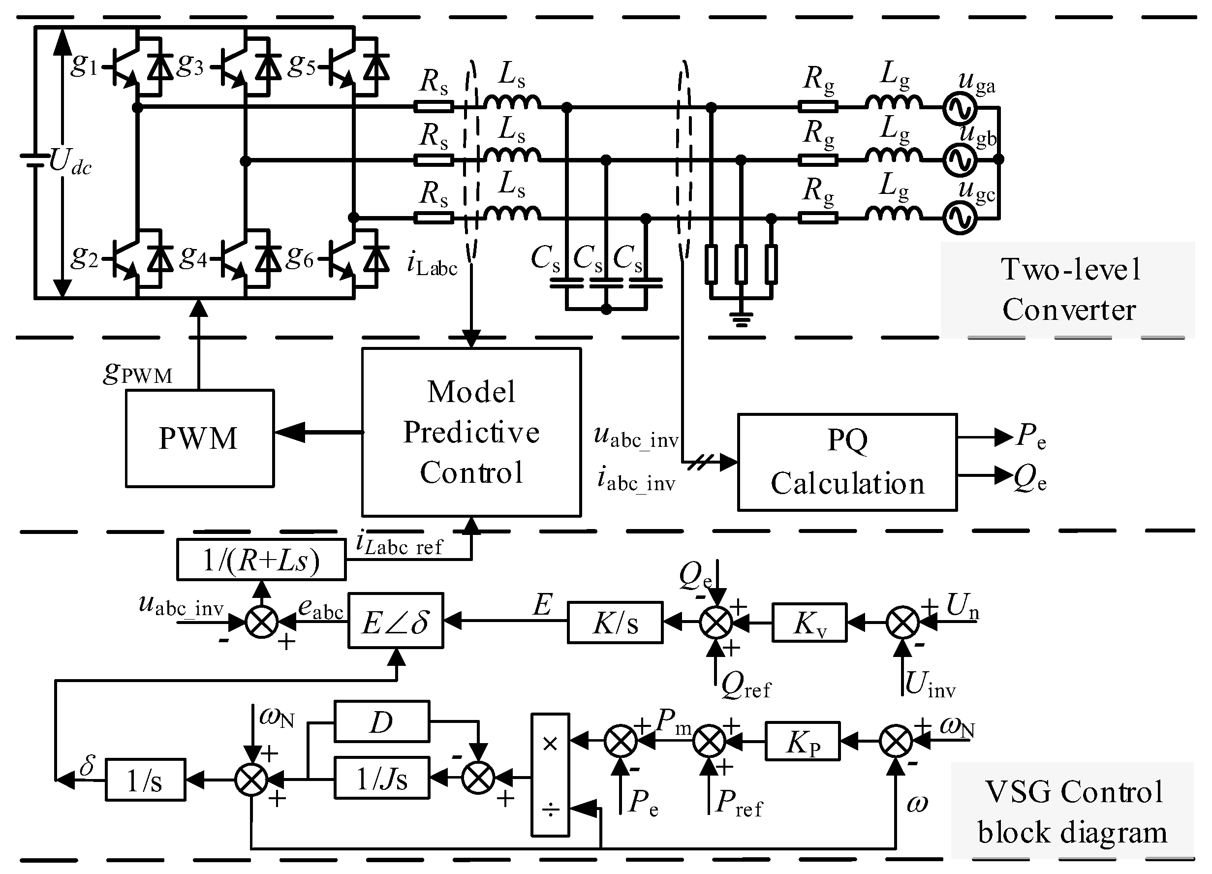
A traditional VSG system is shown in Figure 1. The main circuit of the system consists of a two-level voltage-type converter, where the DC port of the converter is connected to the distributed generation, and the AC output is linked to the load or grid through a filter circuit. The control loop collects the output current, output voltage, and active and reactive power of the main circuit, generates modulation signals through the active-frequency control, reactive-voltage control, and MPC, and finally generates the pulse signal to control the converter. The equivalent diagram and structure diagram of Figure 1: L_s is the filter inductor; C_s is the filter capacitor; P_e and Q_e are the active and reactive power output by the converter, respectively; i_{abc_inv} and u_{abc_inv} are the output current and voltage.

2.2. Mathematical Model of VSG Control

The stator electrical equation and the typical second-order rotor motion equation of the synchronous generator are given in (1).

$$\left\{\begin{array}{l}e=u+i\left(R+\mathrm{j}\omega L\right)\\ T_{\mathrm{m}}-T_{\mathrm{e}}={\displaystyle \frac{P_{\mathrm{m}}-P_{\mathrm{e}}}{\omega }}=J{\displaystyle \frac{d\omega }{dt}}+D\Delta \omega \\ \Delta \omega =\omega -{\omega }_{\mathrm{N}}\\ {\displaystyle \frac{d\delta }{dt}}=\omega \end{array}\right.$$

(1)

In the stator electrical equation, u represents the armature terminal voltage; L denotes the inductance, and R is the stator resistance. In the rotor motion equation, T_m is the mechanical torque; T_e is the electromagnetic torque; J is the moment of inertia; D is the damping coefficient; ω is the mechanical angular velocity; ω_N is the rated angular velocity of the system; δ is the output power angle.

As shown in Figure 1, based on the principles of the synchronous generator governor and excitation regulator, the equation relationships between active power and frequency, as well as reactive power and voltage, are established, as given in (2).

$$\left\{\begin{array}{l}\omega =2\pi f\\ E={\displaystyle \frac{K}{s}}\left[Q_{\mathrm{ref}}+K_{\mathrm{V}}\left(U_{\mathrm{n}}-U_{\mathrm{inv}}\right)-Q_{\mathrm{e}}\right]\\ \Delta T=\left[P_{\mathrm{ref}}+K_{\mathrm{P}}\left({\omega }_{\mathrm{N}}-\omega \right)-P_{\mathrm{e}}\right]/\omega \end{array}\right.$$

(2)

In (2), the reference values for active power and reactive power are denoted as P_ref and Q_ref; K_V, K_P, and K denote the voltage regulation coefficient, the active power droop coefficient, and the integral loop coefficient, respectively. In addition, U_n and U_inv denote the voltage reference and the RMS value of the output voltage, respectively; E is the virtual potential command, and f is the frequency of the VSG output voltage.

Therefore, combining the obtained voltages in the voltage synthesis link reference value and phase angle, the output voltage of VSG is given in (3).

$$\left\{\begin{array}{l}{e}_{\mathrm{a}\_\mathrm{ref}}=\sqrt{2}E\sin \delta \\ e_{\mathrm{b}\_\mathrm{ref}}=\sqrt{2}E\sin \left(\delta -{\displaystyle \frac{2\pi }{3}}\right)\\ e_{\mathrm{c}\_\mathrm{ref}}=\sqrt{2}E\sin \left(\delta +{\displaystyle \frac{2\pi }{3}}\right)\end{array}\right.$$

(3)

Furthermore, the reference value for the output current of VSG be obtained as:

$$\left\{\begin{array}{l}{i}_{L\mathrm{a}\_\mathrm{ref}}={\displaystyle \frac{e_{\mathrm{a}\_\mathrm{ref}}-u_{\mathrm{a}\_\mathrm{inv}}}{R_{\mathrm{s}}+s{L}_{\mathrm{s}}}}\\ i_{L\mathrm{b}\_\mathrm{ref}}={\displaystyle \frac{e_{\mathrm{b}\_\mathrm{ref}}-u_{\mathrm{b}\_\mathrm{inv}}}{R_{\mathrm{s}}+s{L}_{\mathrm{s}}}}\\ i_{L\mathrm{c}\_\mathrm{ref}}={\displaystyle \frac{e_{\mathrm{c}\_\mathrm{ref}}-u_{\mathrm{c}\_\mathrm{inv}}}{R_{\mathrm{s}}+s{L}_{\mathrm{s}}}}\end{array}\right.$$

(4)

2.3. Mathematical Model of MPC

Based on the mathematical model of the topology derived from the VSG control, the inductor currents can be obtained as shown in (5).

$$\left\{\begin{array}{l}{L}_{\mathrm{s}}{\displaystyle \frac{d{i}_{L\mathrm{a}}}{dt}}=e_{\mathrm{a}}-u_{\mathrm{a}\_\mathrm{inv}}-R_{\mathrm{s}}{i}_{L\mathrm{a}}\\ L_{\mathrm{s}}{\displaystyle \frac{d{i}_{L\mathrm{b}}}{dt}}=e_{\mathrm{b}}-u_{\mathrm{b}\_\mathrm{inv}}-R_{\mathrm{s}}{i}_{L\mathrm{b}}\\ L_{\mathrm{s}}{\displaystyle \frac{d{i}_{L\mathrm{c}}}{dt}}=e_{\mathrm{a}}-u_{\mathrm{c}\_\mathrm{inv}}-R_{\mathrm{s}}{i}_{L\mathrm{c}}\end{array}\right.$$

(5)

In (5), e_abc represents the output voltages of the two-level converter, and their values are determined by the switching signals.

Applying the Clarke transform to (5) and discretizing it, the predictive model for the current is obtained as illustrated in (6), where T_s represents the control period.

$$\left\{\begin{array}{l}{i}_{L\alpha }\left(k+1\right)={\displaystyle \frac{T_{\mathrm{s}}}{L_{\mathrm{s}}}}\left(e_{\alpha }-u_{\alpha \_\mathrm{inv}}\right)+\left(1-{\displaystyle \frac{R_{\mathrm{s}}{T}_{\mathrm{s}}}{L_{\mathrm{s}}}}\right)i_{L\alpha }\left(k\right)\\ i_{L\beta }\left(k+1\right)={\displaystyle \frac{T_{\mathrm{s}}}{L_{\mathrm{s}}}}\left(e_{\beta }-u_{\beta \_\mathrm{inv}}\right)+\left(1-{\displaystyle \frac{R_{\mathrm{s}}{T}_{\mathrm{s}}}{L_{\mathrm{s}}}}\right)i_{L\beta }\left(k\right)\end{array}\right.$$

(6)

Applying the Clark transform to (4) yields the current references i_{Lα_ref} and i_{Lβ_ref}. Therefore, the cost function can be obtained as:

$$G=\left|i_{L\alpha }\left(k+1\right)-i_{L\alpha \_\mathrm{ref}}\right|+\left|i_{L\beta }\left(k+1\right)-i_{L\beta \_\mathrm{ref}}\right|$$

(7)

3. Hybrid Multi-Vector Model Predictive Control

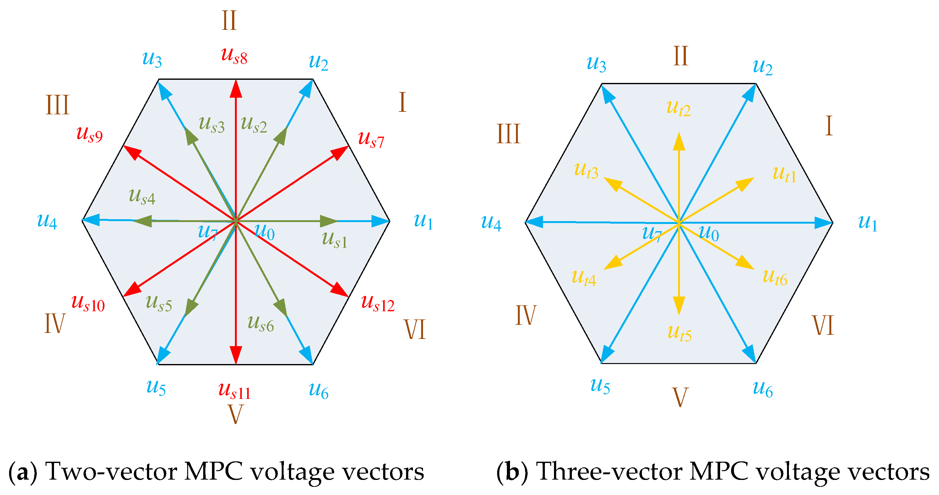
3.1. Two-Vector MPC and Three-Vector MPC Voltage Vectors

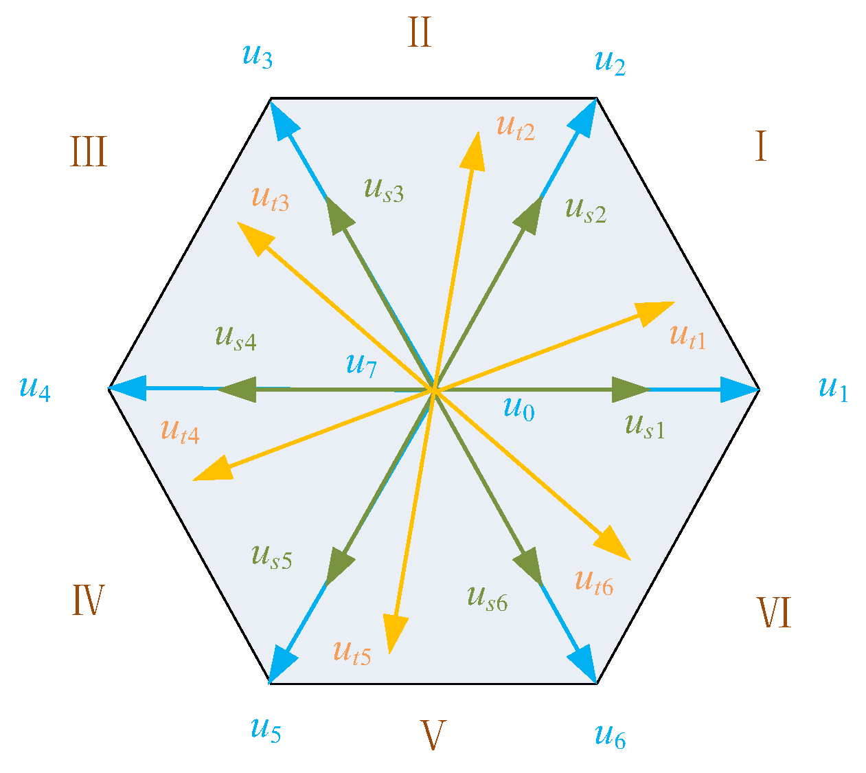
Based on the voltage vector schematic in Figure 2, the voltage vectors for both the two-vector MPC and the three-vector MPC control can be derived. In two-vector MPC, the voltage vector can be divided into real vectors and virtual vectors. The real vectors consist of u_s1(u₀, u₁), u_s2(u₀, u₂), u_s3(u₀, u₃), u_s4(u₀, u₄), u_s5(u₀, u₅), and u_s6(u₀, u₆), while the virtual vectors include u_s7(u₁, u₂), u_s8(u₂, u₃), u_s9(u₃, u₄), u_s10(u₄, u₅), u_s11(u₅, u₆), and u_s12(u₆, u₁). In three-vector MPC, the voltage vectors include u_t1(u₀, u_1, u₂), u_t2(u₀, u₂, u₃), u_t3(u₀, u₃, u₄), u_t4(u₀, u₄, u₅), u_t5(u₀, u₅, u₆), and u_t6(u₀, u₆, u₁).

First, the two-vector MPC is analyzed. Taking u_s1 as an example, it is formed by the combination of u₀ and u₁, so the relationship between the three vectors can be obtained as shown in (8), where t_u0 and t_u1 represent the durations of u₀ and u₁, respectively.

$${\mathit{u}}_{\mathbf{s}\mathbf{1}}={\displaystyle \frac{t_{u_0}}{T_{\mathrm{s}}}}{\mathit{u}}_{\mathbf{0}}+{\displaystyle \frac{t_{u_1}}{T_{\mathrm{s}}}}{\mathit{u}}_{\mathbf{1}}$$

(8)

The duration of each voltage vector should be inversely proportional to its corresponding cost function. Therefore, based on the cost function values G_u0 and G_u1 corresponding to u₀ and u₁, the durations of t_u0 and t_u1 are given in (9).

$$\left\{\begin{array}{l}{t}_{u0}={\displaystyle \frac{G_{u1}}{G_{u0}+G_{u1}}}{T}_s\hfill \\ t_{u1}={\displaystyle \frac{G_{u0}}{G_{u0}+G_{u1}}}{T}_s\hfill \end{array}\right.$$

(9)

Similarly, the relationship between the virtual vectors and the fundamental vectors in the three-vector MPC can also be derived. Taking u_t1 as an example, the durations of u₀, u₁, and u₂ are given in (10), where G_u0, G_u1, and G_u2 represent the values of the corresponding cost functions for these vectors, respectively.

To compare the two-vector MPC and three-vector MPC, the vector corresponding to sector 1 is selected as an example for the cost function calculation. According to [27], in the two-vector MPC, the cost function expressions corresponding to the three vectors u_s1, u_s2, and u_s7 are given in (11), while the cost function expressions corresponding to the three-vector MPC are provided in (12). In (11) and (12), the vectors u_αref and u_βref represent the components of the voltage vector u_αβref in the αβ co-ordinate system.

$$\left\{\begin{array}{l}{t}_{u0}={\displaystyle \frac{G_{u1}{G}_{u2}}{G_{u0}{G}_{u1}+G_{u1}{G}_{u2}+G_{u0}{G}_{u2}}}{T}_s\hfill \\ t_{u1}={\displaystyle \frac{G_{u0}{G}_{u2}}{G_{u0}{G}_{u1}+G_{u1}{G}_{u2}+G_{u0}{G}_{u2}}}{T}_s\hfill \\ t_{u2}={\displaystyle \frac{G_{u0}{G}_{u1}}{G_{u0}{G}_{u1}+G_{u1}{G}_{u2}+G_{u0}{G}_{u2}}}{T}_s\hfill \end{array}\right.$$

(10)

$$\left\{\begin{array}{l}{G}_{us1}=\left|{\mathit{u}}_{\alpha \mathrm{ref}}-{\displaystyle \frac{2}{3}}{\displaystyle \frac{G_{u0}{\mathit{U}}_{\mathrm{dc}}}{G_{u1}+G_{u0}}}\right|+{\mathit{u}}_{\beta \mathrm{ref}}\\ G_{us2}=\left|{\mathit{u}}_{\alpha \mathrm{ref}}-{\displaystyle \frac{1}{3}}{\displaystyle \frac{G_{u7}{\mathit{U}}_{\mathrm{dc}}}{G_{u7}+G_{u2}}}\right|+\left|{\mathit{u}}_{\beta \mathrm{ref}}-{\displaystyle \frac{\sqrt{3}}{3}}{\displaystyle \frac{G_{u7}{\mathit{U}}_{\mathrm{dc}}}{G_{u7}+G_{u2}}}\right|\\ G_{us7}=\left|{\mathit{u}}_{\alpha \mathrm{ref}}-{\displaystyle \frac{1}{3}}{\displaystyle \frac{G_{u1}{\mathit{U}}_{\mathrm{dc}}}{G_{u1}+G_{u2}}}-{\displaystyle \frac{2}{3}}{\displaystyle \frac{G_{u2}{\mathit{U}}_{\mathrm{dc}}}{G_{u1}+G_{u2}}}\right|+\left|{\mathit{u}}_{\beta \mathrm{ref}}-{\displaystyle \frac{\sqrt{3}}{3}}{\displaystyle \frac{G_{u1}{\mathit{U}}_{\mathrm{dc}}}{G_{u1}+G_{u2}}}\right|\end{array}\right.$$

(11)

$$\left\{\begin{array}{l}{G}_{ut1}=\left|{\mathit{u}}_{\alpha \mathrm{ref}}-{\displaystyle \frac{2}{3}}{\displaystyle \frac{G_{u0}{G}_{u2}{\mathit{U}}_{\mathrm{dc}}}{f}}-{\displaystyle \frac{1}{3}}{\displaystyle \frac{G_{u0}{G}_{u1}{\mathit{U}}_{\mathrm{dc}}}{f}}\right|+\left|{\mathit{u}}_{\beta \mathrm{ref}}-{\displaystyle \frac{\sqrt{3}}{3}}{\displaystyle \frac{G_{u0}{G}_{u1}{\mathit{U}}_{\mathrm{dc}}}{f}}\right|\\ f=G_{u0}{G}_{u1}+G_{u2}{G}_{u1}+G_{u0}{G}_{u2}\end{array}\right.$$

(12)

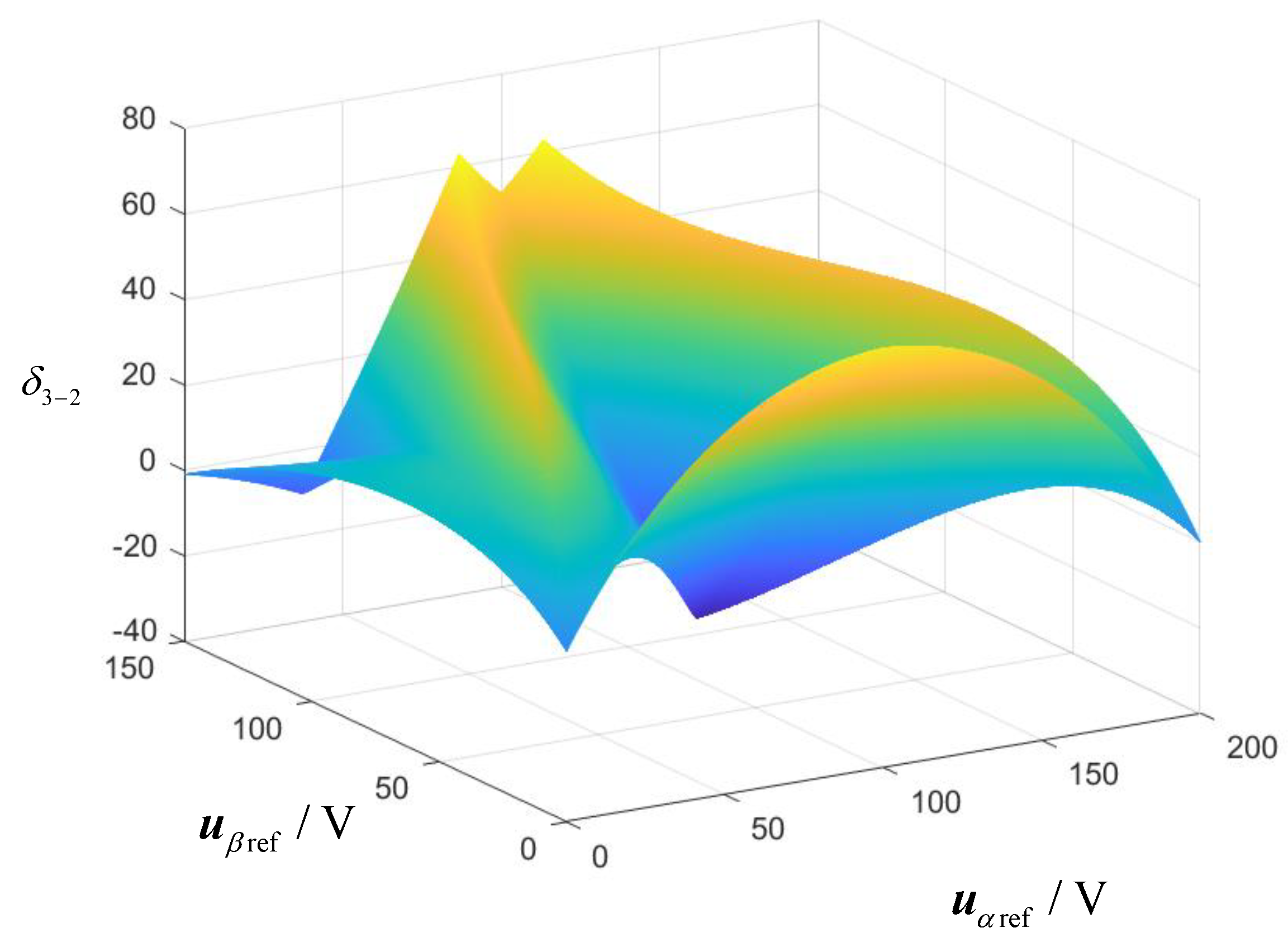
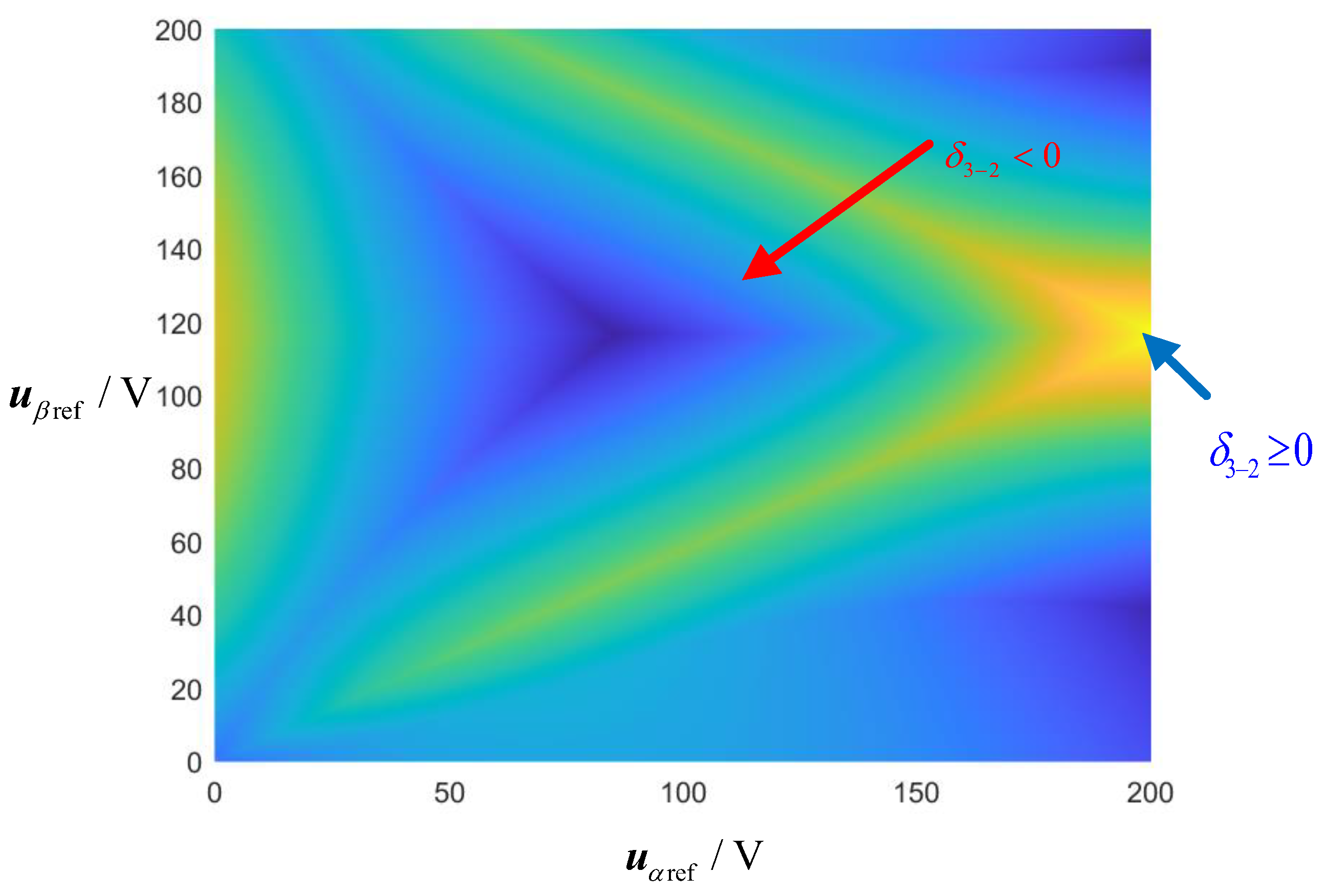
The two control strategies are compared by analyzing the differences in their cost functions. The expression for the difference is provided in (13), and its waveform is shown in Figure 3. As can be seen, the value of δ_3-2 is greater than 0 under certain conditions, indicating that the performance of the three-vector MPC is not universally superior to that of the two-vector MPC. The two-vector MPC is more effective when the reference voltage vector is near the edge of each sector, while the three-vector MPC performs better when the reference voltage is farther from the edge of each sector. Therefore, optimal control cannot be achieved by using either the two-vector MPC or the three-vector MPC alone.

$${\delta }_{3-2}=G_{ut1}-\min \left(G_{us1},G_{us2},G_{us7}\right)$$

(13)

3.2. Hybrid Multi-Vector MPC

The analysis of the two-vector MPC and three-vector MPC indicates that, for optimal control, the optimal voltage vector should be selected from u_s1 to u_s12 when the reference voltage is near the edge of each sector, and from u_t1 to u_t6 when the reference voltage is farther from the edge of the sector. Therefore, the hybrid multi-vector MPC is proposed by combining the two-vector MPC and three-vector MPC to achieve optimal voltage vector selection for each control period.

As shown in Figure 2, the two-vector MPC consists of twelve voltage vector sets, while the three-vector MPC consists of 6 voltage vector sets. If these two types of control are directly combined as in [27], 18 voltage vector sets would need to be calculated in each control cycle, which places higher demands on the controller. Therefore, it is necessary to analyze these 18 voltage vector sets.

By comparing the virtual vectors in the two-vector MPC with the vectors in the three-vector MPC, it can be observed that u_t1 contains one additional zero vector compared to u_s7. The voltage vectors u_t1 and u_s7 are equivalent when the action time of the zero vector is zero, meaning u_t1 can be considered to contain u_s7. Similarly, it can be argued that u_t2, u_t3, u_t4, u_t5 and u_t6 contain u_s8, u_s9, u_s10, u_s11, and u_s12, respectively. Therefore, 12 sets of voltage vectors (u_s1, u_s2, u_s3, u_s4, u_s5, u_s6, u_t1, u_t2, u_t3, u_t4, u_t5, and u_t6) are selected to compute the cost function in the proposed hybrid multi-vector MPC. Therefore, the cost function needs to be computed only 12 times in each control period, reducing the number of calculations by 1/3 compared to the method proposed by [27]. The voltage vector combinations in the proposed hybrid multi-vector MPC are shown in Figure 4.

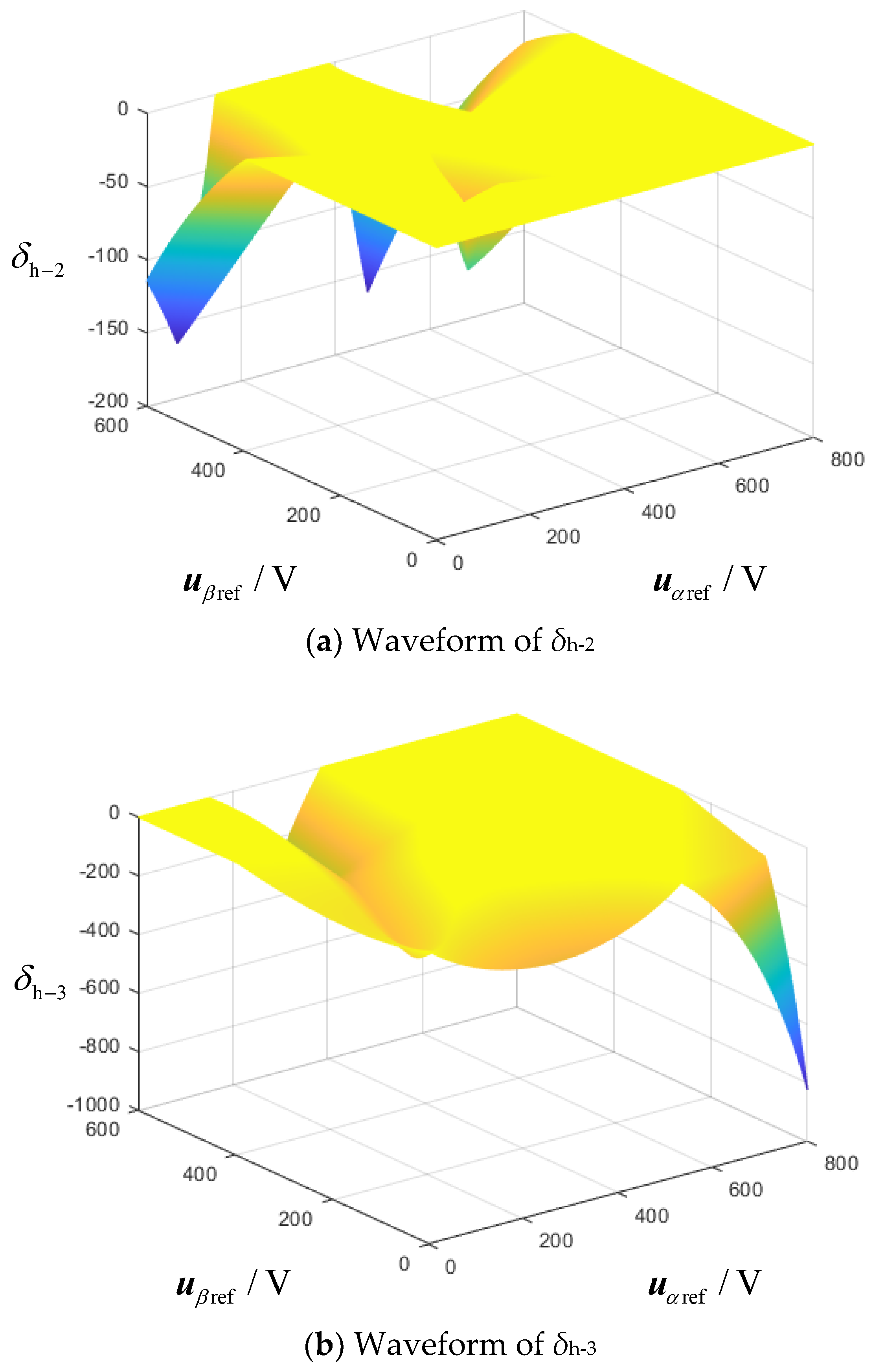
To further demonstrate that the proposed hybrid multi-vector MPC effectively reduces the harmonic content of the current, its cost functions are compared with those of the two-vector MPC and the three-vector MPC. The comparison is presented using sector 1 as an example. The difference in the cost function between the hybrid multi-vector MPC and the two-vector MPC, as well as the three-vector MPC, is defined as δ_h-2 and δ_h-3, respectively, as shown in (14). It should be noted that when the value of G_u0 equals to 1, the value of f equals to G_u1 + G_u2, and the remaining moments of f are shown in (12).

$$\left\{\begin{array}{l}{\delta }_{\mathrm{h}-2}=\min \left(G_{us1},G_{us2},G_{ut1}\right)-\min \left(G_{us1},G_{us2},G_{us7}\right)\hfill \\ {\delta }_{\mathrm{h}-3}=\min \left(G_{us1},G_{us2},G_{ut1}\right)-G_{ut1}\hfill \end{array}\right.$$

(14)

The waveforms of δ_h-2 and δ_h-3 are shown in Figure 5. As observed, both δ_h-2 and δ_h-3 are consistently less than 0, indicating that the proposed hybrid multi-vector MPC effectively reduces the current harmonics compared to the two-vector MPC and three-vector MPC.

A comparison is conducted among the traditional dual-loop control, single-vector MPC, two-vector MPC, three-vector MPC, and the proposed hybrid multi-vector MPC under the same operating conditions, and the details are provided in

Table 1. Comparison of the dual-loop control, two-vector MPC, three-vector MPC, and proposed MPC.

	Dual-loop Control	Single-Vector MPC	Two-Vector MPC	Three-Vector MPC	Hybrid Multi-Vector MPC
Dynamic response time	long	short	short	short	short
Current harmonic content	\	high	medium	medium	low

. In terms of dynamic response time, the dual-loop control has a longer dynamic response time, while the four MPC methods exhibit shorter dynamic response times. Then, the current harmonic content among these methods is compared. Since the output current of the traditional dual-loop control is determined by the proportional and integral parameters of the inner loop, it will not be compared with the other MPC methods. As previously analyzed, the harmonic content of the output current is highest in the single-vector MPC method. Both the two-vector MPC and three-vector MPC methods improve the harmonic content of the output current compared to the single-vector MPC. However, these two methods cannot achieve optimal current output in all cases. In contrast, the proposed hybrid multi-vector MPC achieves the lowest output current harmonic content in all cases.

3.3. Considering Frequency Variation in Cost Function

In microgrids, frequency is sensitive to load changes: an increase in load causes a temporary drop in frequency, while a decrease in load results in a temporary rise in frequency. Traditional MPC approaches typically focus only on the output current, ignoring frequency variations. To address this, this paper proposes an MPC strategy that incorporates frequency variation into the control process.

The rotor motion equation in VSG control is given in (15), where K_p is the sag coefficient.

$$\left\{\begin{array}{l}{P}_{\mathrm{m}}=P_{\mathrm{ref}}-K_{\mathrm{p}}\left(\omega -{\omega }_{\mathrm{N}}\right)\\ P_{\mathrm{m}}-P-D{\omega }_{\mathrm{N}}\Delta \omega =J\omega {\displaystyle \frac{d\omega }{dt}}\approx J{\omega }_{\mathrm{N}}{\displaystyle \frac{d\omega }{dt}}\end{array}\right.$$

(15)

Discretizing (15) results in a discrete model of the angular frequency, as shown in (16).

$$\omega \left(k+1\right)={\displaystyle \frac{T_{\mathrm{S}}}{J{\omega }_N}}\left[P_{\mathrm{ref}}-P+\left(K_p+D{\omega }_N\right){\omega }_N\right]+\left[1-{\displaystyle \frac{T_{\mathrm{S}}}{J{\omega }_N}}\left(K_p+D{\omega }_N\right)\right]\omega \left(k\right)$$

(16)

Based on (16), the angular frequency at time step k + 1 can be computed. Therefore, the deviation of this angular frequency can be incorporated into the cost function. The expression for the modified cost function is given in (17), where k_f is the weighting factor for frequency variation. The value of k_f can be adjusted based on the magnitude of the frequency deviation. When the frequency deviation is small, k_f can be to 0.

$$G=\left|i_{L\alpha }\left(k+1\right)-i_{L\alpha \_\mathrm{ref}}\right|+\left|i_{L\beta }\left(k+1\right)-i_{L\beta \_\mathrm{ref}}\right|+k_{\mathrm{f}}\left|\omega \left(k+1\right)-{\omega }_{\mathrm{N}}\right|$$

(17)

4. Simulation Analysis

To verify the effectiveness of the proposed hybrid multi-vector MPC, a two-level VSG model is developed in the MATLAB/Simulink platform, and the relevant control parameters used are shown in

Table 2. Simulation parameters of VSG.

Parameter	Numerical Value	Parameter	Numerical Value
Rated voltage on AC grid ug (V)	380	Filter inductor Ls (mH)	2.2
Rated voltage on DC side Udc (V)	800	Filter capacitor Cs (uF)	20
Rated active power (kW)	50	Grid-side inductance Lg (mH)	1
Rated reactive power (Var)	0	Control period Ts (ms)	0.1

.

The system operates in a grid-connected state with a simulation duration of 2 s. The microgrid has a rated frequency of 50 Hz and grid-connected active power of 50 kW, while the reactive power remains constant at 0 kVar during this period. The two-vector MPC, three-vector MPC, and the proposed hybrid multi-vector MPC are compared under two operating conditions: power variation and frequency variation. In the power variation condition, the grid-connected power increases by 10 kW at 1 s, while in the frequency variation condition, the microgrid frequency increases by 0.2 Hz at 1 s.

4.1. Power Variation Condition

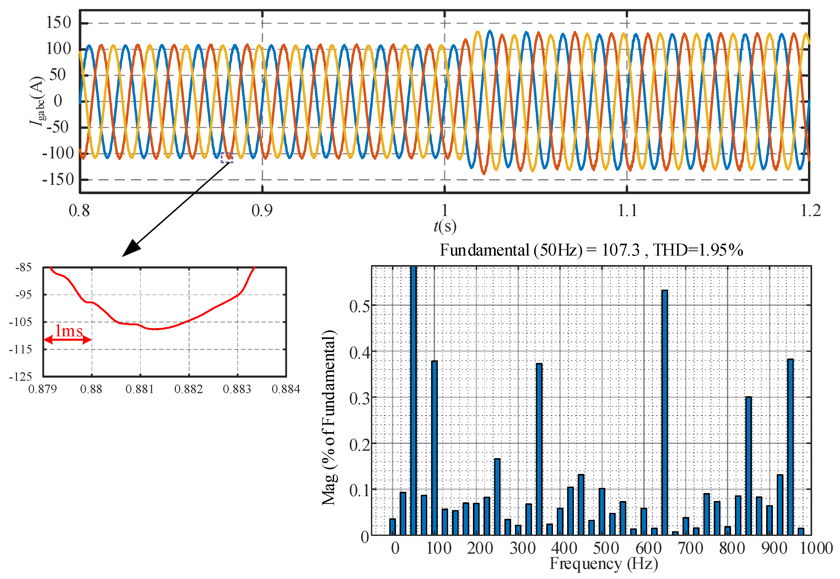
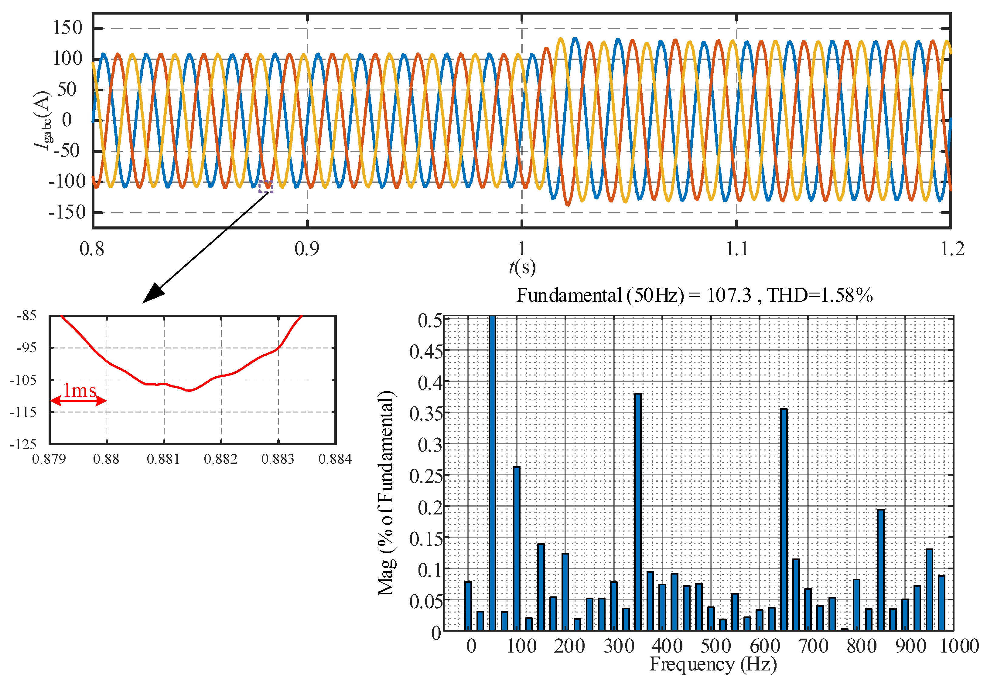
The simulation results of the two-vector MPC, three-vector MPC, and the proposed hybrid multi-vector MPC under varying power conditions are shown in Figure 6, Figure 7 and Figure 8. As can be seen from Figure 6, with the two-vector MPC, the ripple current of the converter is large, and the total harmonic content reaches 2.49%. Compared to the two-vector MPC, the ripple current of the converter is significantly improved with the three-vector MPC, as shown in Figure 7, and the total harmonic content is reduced to 1.95%. In addition, as shown in Figure 8, the ripple current of the converter can be further reduced by using the proposed hybrid multi-vector MPC, and the total harmonic content is decreased to 1.54%. This is consistent with the previous theoretical analyses.

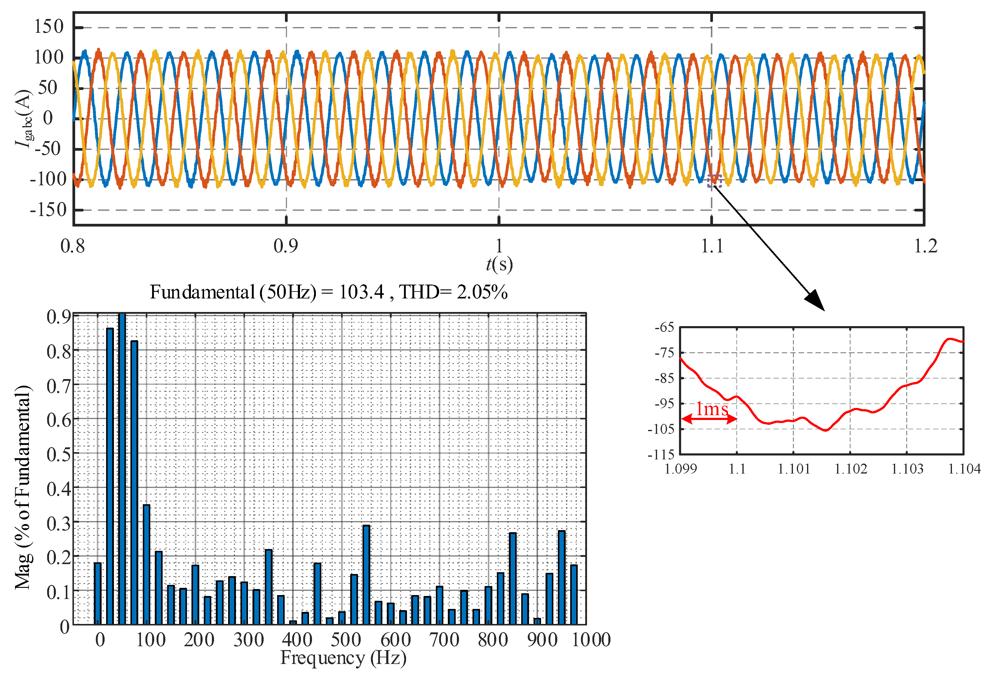
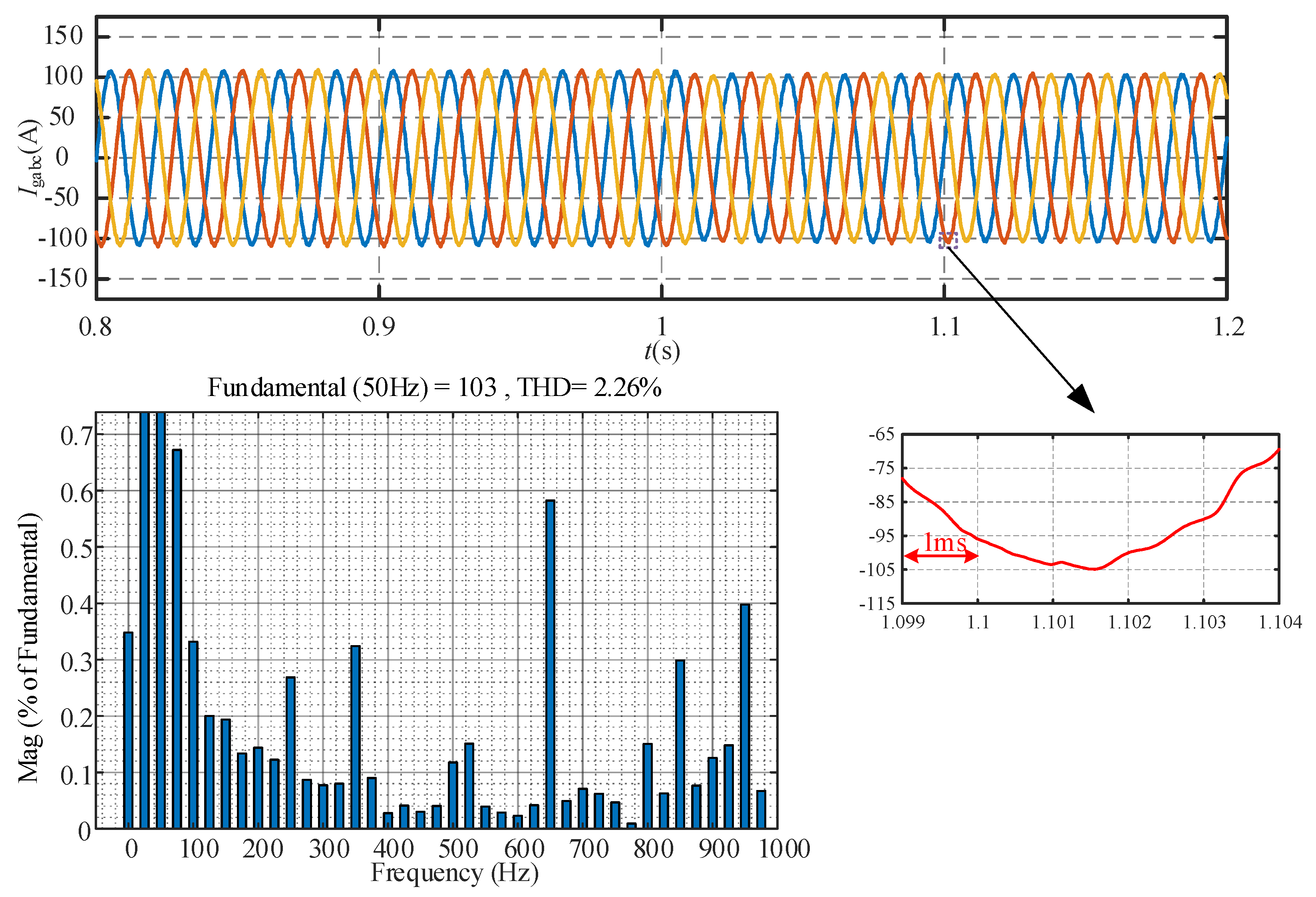
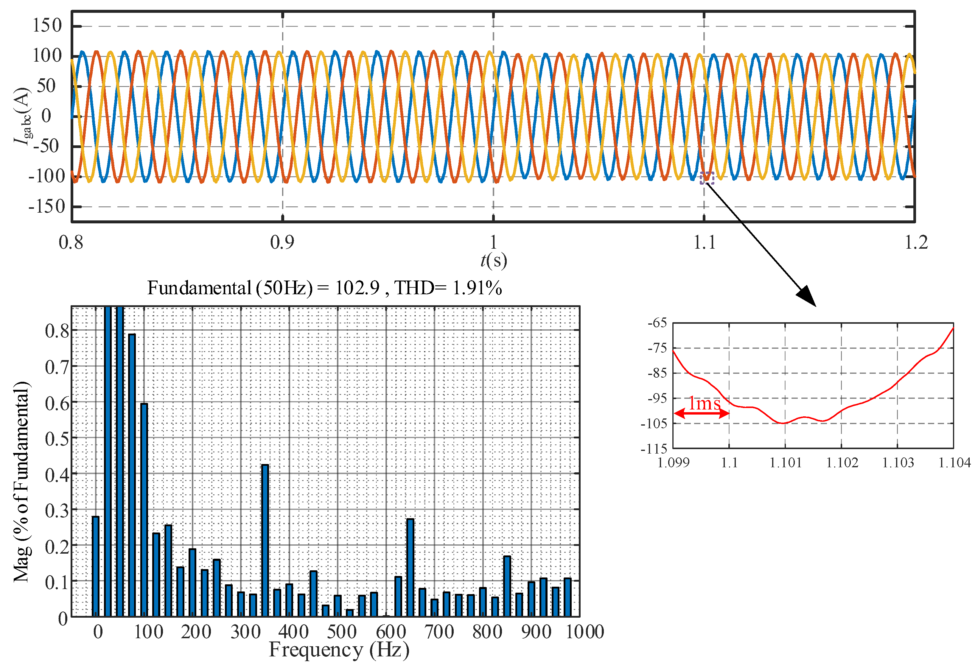
4.2. Frequency Variation Condition

The simulation results for the two-vector MPC, three-vector MPC, and hybrid multi-vector MPC under varying frequency conditions are shown in Figure 9, Figure 10 and Figure 11. The simulation results show that after the frequency change, the total harmonic content of the current measured by the three methods is 2.05%, 2.26%, and 1.91%, respectively. When using the proposed hybrid multi-vector MPC, the total harmonic content of the converter output current remains the lowest. Additionally, the total harmonic content of the output current with the two-vector MPC is lower than that with the three-vector MPC. Therefore, based on the simulation results presented in Figure 6, Figure 7, Figure 9, and Figure 10, it can be observed that neither the two-vector MPC nor the three-vector MPC alone can achieve the lowest harmonic content of the output current under different operating conditions, which is consistent with the previous theoretical analysis.

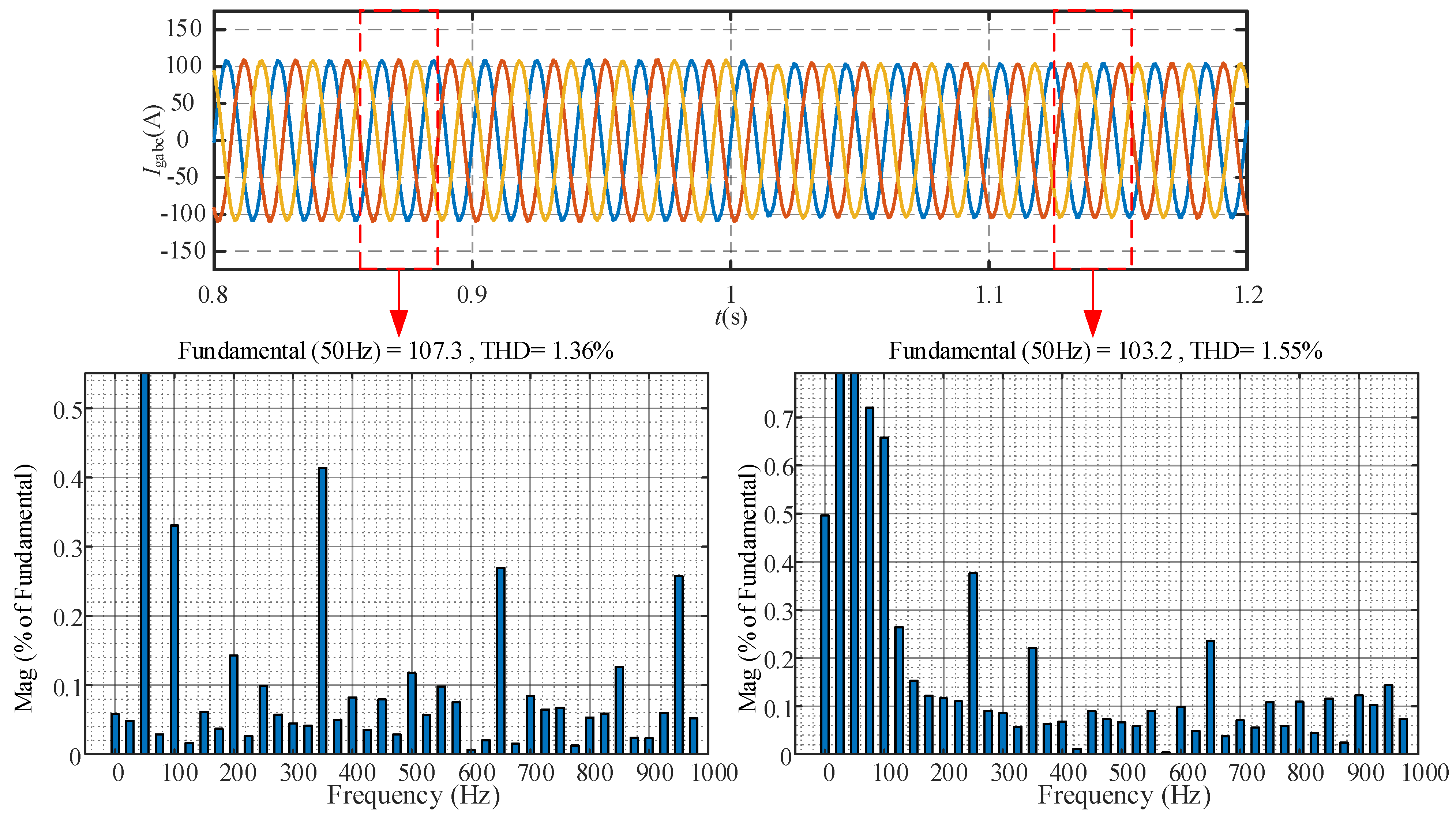
The simulation results of the hybrid multi-vector MPC, which incorporates frequency variation into the cost function, are presented in Figure 12. In the simulation, the value of k_f is set to 0 when the frequency variation in the system is within 0.05 Hz, and the value of k_f is set to 1 when the frequency variation exceeds 0.05 Hz. From the simulation results, it can be observed that when the microgrid frequency is 50 Hz, the harmonic content of the output current is slightly improved compared to the results shown in Figure 9, using the hybrid multi-vector MPC that accounts for frequency variation. When the microgrid frequency is increased by 0.2 Hz, the harmonic content of the output current is only 1.55%, nearly 20% lower than the results shown in Figure 12.

5. Conclusions

VSG technology enhances system stability by simulating the characteristics of synchronous generators. However, conventional two-vector MPC and three-vector MPC cannot guarantee that the optimal voltage vector, which minimizes current harmonic content, is selected in every control period. To address this issue, this paper proposes a hybrid multi-vector MPC strategy. The effectiveness of this approach is validated through simulations involving power variation and frequency variation. The main contributions of this work are as follows:

(1)

The cost functions of two-vector MPC and three-vector MPC are analyzed, and it is shown that neither control strategy can achieve the global optimum for minimizing the harmonic content of the converter output current.

(2)

A hybrid multi-vector MPC strategy is proposed that introduces a new combination of vectors, enabling the selection of the voltage vector with the lowest current harmonic content in each control period, without increasing the number of iterations.

(3)

A hybrid multi-vector MPC strategy that considers frequency variations is proposed to further improve the quality of the output current by incorporating frequency variation weighting coefficients into the cost function.