Article

Application of State Models in a Binary–Temporal Representation for the Prediction and Modelling of Crude Oil Prices

by
Michał Dominik Stasiak
1,*,
Żaneta Staszak
2,
Joanna Siwek
3 and
Dawid Wojcieszak
4
1
Department of Investment and Real Estate, Poznań University of Economics and Business, al. Niepodleglosci 10, 61-875 Poznań, Poland
2
The Faculty of Civil and Transport Engineering, Poznan University of Technology, 5 M. Skłodowska-Curie Square, 60-965 Poznań, Poland
3
Faculty of Mathematics and Computer Science, Department of Artificial Intelligence, Adam Mickiewicz University, Uniwersytetu Poznańskiego 4, 61-614 Poznań, Poland
4
Department of Biosystems Engineering, Poznań University of Life Sciences, ul. Wojska Polskiego 50, 60-627 Poznań, Poland
*
Author to whom correspondence should be addressed.
Energies 2025, 18(3), 691; https://doi.org/10.3390/en18030691
Submission received: 4 January 2025 / Revised: 25 January 2025 / Accepted: 27 January 2025 / Published: 2 February 2025
(This article belongs to the Section C: Energy Economics and Policy)

Abstract

:
Crude oil prices have a key meaning for the economies of most countries. Their levels shape the general production costs in many sectors. Oil prices are also a base for financial derivatives like CFD contracts, which are popular nowadays. Due to these reasons, the possibility of an effective prediction of the direction of future changes in the price of crude oil is especially significant. Most existing works focus on the analysis of daily closing prices. This kind of approach results, on the one hand, in losing important information about the dynamics of changes during the day. On the other hand, it does not allow for the modelling of short-term price changes that are especially important in cases of financial derivatives having crude oil as their base instrument. The goal of the following article is the analysis of possible applications of a binary–temporal representation in the modelling and construction of effective decision support systems on the crude oil market. The analysis encompasses all researched state models, e.g., those applying mean and trend analysis. Also, the selection of parameters was optimized for Brent crude oil rates. The presented research confirms the high effectiveness of our state modelling system in predicting oil prices on a level that allows for the construction of financially effective investment decision support systems. The obtained results were verified based on proper backtests from different quotation periods. The presented results can be used both in scientific analyses and in the construction of investment support tools for the crude oil market.

1. Introduction

The crude oil market is one of the biggest markets in the world. The price of this resource influences energy costs and the costs of all land, sea and air transportation. Crude oil is also crucial for the chemical industry. Fluctuations in oil prices directly influence the shapes and conditions of whole economies [1,2]. Oil rates are also the basis for many financial derivatives, such as CFD (Contract for Difference) contracts [3]. Due to the importance of crude oil prices for economies and investors, the development of adequate methods for predicting direction changes in price trajectory for crude oil quotations is a difficult and impactful challenge.
Most of the current research focuses on the prediction of long-term changes in crude oil price trajectories. In the literature, it is difficult to find works that pertain to the construction of tools that support short-term investors. Similarly, works describing transaction automatization with the use of derivatives are scarce. This article fills both of those niches.
In [4], the authors proved the applicability of a state modelling approach in the binary–temporal representation of crude oil prices with the use of the state model of the binary trend (SMBT), constructed for arbitrarily selected parameters. In this work, the authors also conducted research on the following: a state model of a binary representation (SMBR); a state model of a binary–temporal representation (SMBRT); and a state model of the binary moving average (SMBMA); as well as performed the optimization of parameter selection, considering financial effectiveness. In order to conduct this research, dedicated software was created in the C++ and MQL4 languages, optimized for repetitive computing of large volumes of data. This research used tick data for Brent crude oil price, expressed in American dollars (Brent/USD), taken from the Swiss Ducascopy broker over a period of 6 years.
The results of this research, as described in this article, indicate a high effectiveness of the used prediction state models based on trend analysis and mean analysis of the oil market. As a consequence, the models allow for the construction of financially effective algorithmic trade systems. The obtained results also allow for the optimal selection of parameters for the crude oil market. The parameters can be then used for both assessing the direction of future changes in oil prices and the full automatization of the trade on this market.
This paper is organized as follows: After the brief introduction, Section 2 contains a literature review, introducing the current state of the research on the described topic. Section 3 shows the concept and advantages of the binary–temporal representation. Section 4 relates the model assumptions for state modelling and details the construction of the applied state models. This section also presents exemplary modelling results for crude oil prices in each of the beforementioned models. Section 5 summarizes the optimization results and the practical implementation of the state models on the oil market. This paper ends with a summary of the obtained results.

2. Literature Overview

Due to the high importance of oil prices for the global market, many works focus on the influence of oil prices on particular sectors of the economy [5,6]. The results of this kind of research justify the need to construct tools for predicting the direction of future changes in the oil price trajectory. The majority of the works pertain to price analysis using candlestick representation. The data usually consist of daily closing prices, which are generally considered to have the potential for creating long-term price forecasts [7,8,9,10,11,12,13]. Omitting information about price fluctuations during the day can lead to less effective modelling since in-day fluctuations can influence the probability of future changes in the price trajectory. Another consequence of this approach is the limited possibility of applying the results in the derivative market, such as CFD contracts, where investors open and close the transactions in a very short time (e.g., hours) [14,15].
Nowadays, due to the rapid development of advanced IT solutions, the popularity of support or automatic trade systems is constantly increasing [16]. Systems of these kinds are characterized by many advantages and are expected to increase in significance on exchange and financial markets, including the crude oil market. Therefore, a large amount of research in the last few years has focused on automatic oil trade systems [17,18]. Yet, in the existing literature, according to the authors’ best knowledge, there are no works in which the modelling method used allows for an unequivocal selection of the Take profit and Stop loss levels, which directly influence the financial effectiveness of the algorithmic trade systems. The introduced models that use binary–temporal data representation and state modelling allow for filling this research gap.
The first studies on binary–temporal representation identified the disadvantages of the candlestick representation and proposed an alternative [19]. Subsequently, based on the introduced binary–temporal representation, additional models were examined, including SMBTR [20], SMBMA [21] and SMBT [4]. The application of state modelling to this type of data for oil price modelling was verified only for the SMBT model, yielding positive results. The feasibility of constructing financially effective systems was demonstrated. However, these results were obtained using an arbitrarily chosen set of parameters. In this article, we verify the applicability of the remaining models and optimize parameter selection to determine which model, along with its corresponding parameters, can be used to develop the most financially effective tools for supporting investment decisions in the crude oil market.

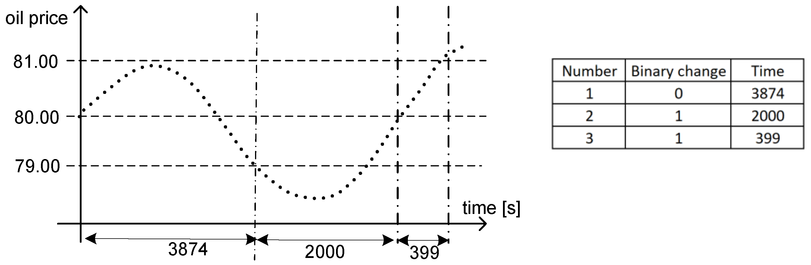
3. Representation of Crude Oil Rates

Most of the works on the researched topic, as well as those pertaining exactly to the oil market, are dominated by the candlestick representation of historical data that is used in analysis. The price movement given in this form is described, for each time period, by four values: the opening, closing, minimum and maximum prices [22,23,24]. This format leads to losing information about the changes in the price trajectory “inside the candle” (see Figure 1). Additionally, in many studies, an even more truncated format is used, with only closing prices considered as data for analyses. In the case of crude oil, research with only daily closing prices considered strongly dominates the literature. Using this form of data that loses so much information about the price variability can significantly lower the quality and credibility of modelling. A detailed description of the binary–temporal representation and the consequences of using the candlestick chart representation can be found in [19].
The binary–temporal representation was inspired by the point-symbolic method [25]. In this representation, the price movement is given as a series of binary values representing an increase ( ε i = 1) or decrease ( ε i = 0) in the price by a given value δ known as the discretization unit, which is expressed in pips. Each change in the price value is assigned its duration, given in seconds ( Δ t i ) . The historical trajectory can therefore be written in the form of a series given by the formula:
B T = { ( ε i ,   Δ t i ) } i = 1 N .
The main function of the binary–temporal representation is noise filtration [26,27]. By setting a given precision, only changes within a preset range will be registered, with the range being defined by the value of the discretization unit. This kind of representation can not only be effectively used to model price trajectories, but it is also easier to interpret.

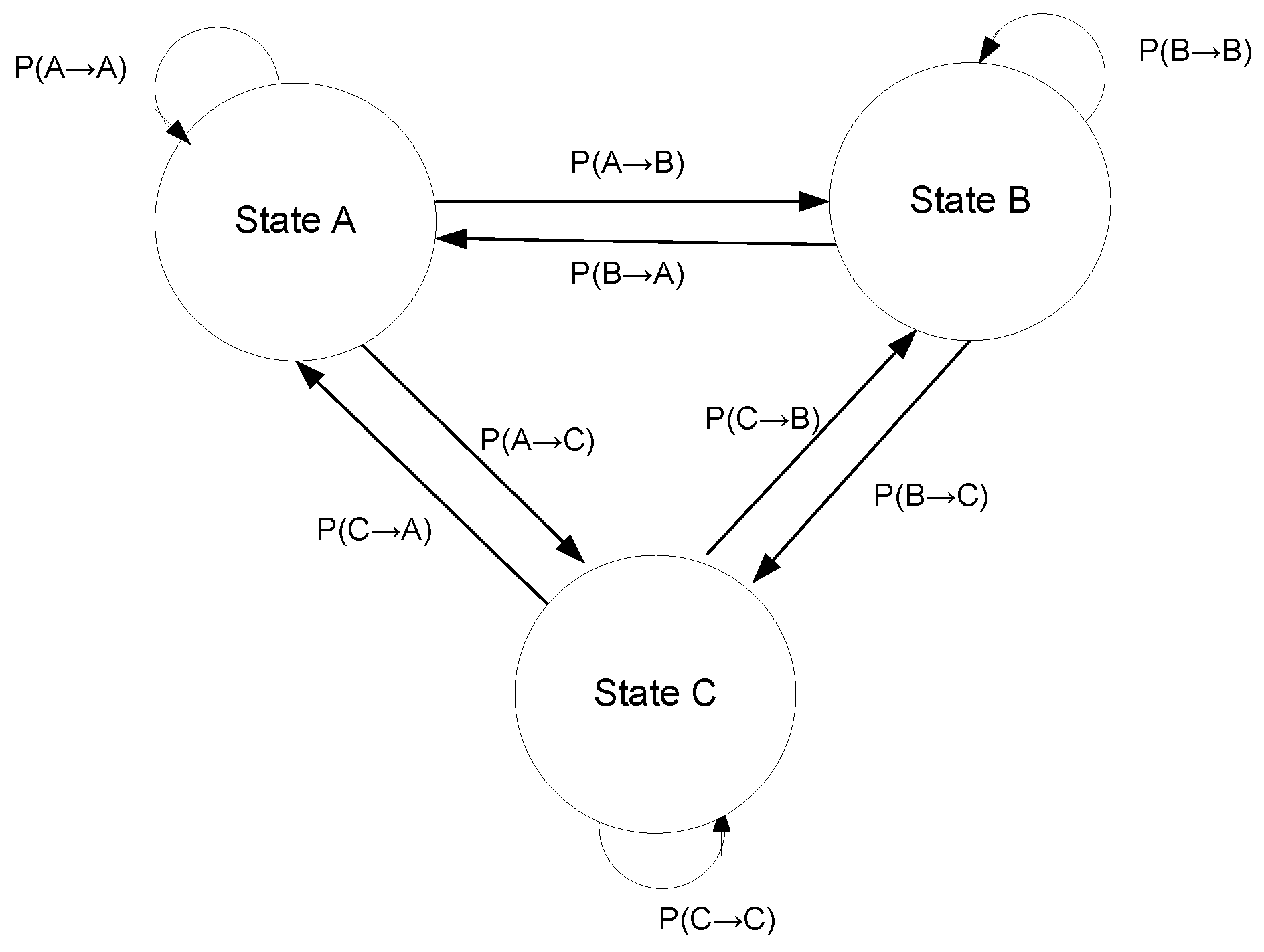
4. Modelling of Crude Oil Rates Using State Models in a Binary–Temporal Representation

Assumptions of State Modelling

State modelling is a part of technical analysis and uses the basic concept of searching for statistically recurring behaviour patterns in investors’ market activity. The existence of these kinds of patterns has been thoroughly researched and proven with statistical methods and justified by adequate psychological analyses performed on investors.
The main assumption of the state modelling of the price in a binary–temporal representation is the definition of market states and the assignment of probability distributions of transitions between the states. These transitions can be interpreted as a recurring and statistically significant behaviour patterns among investors. As a result, based on state modelling, we can describe the probabilistic distribution of decreases/increases that occur in the price trajectory as a reaction to a given state of the market. A general, exemplary schema of a state model can be found in Figure 2. The obtained probability distribution can be used for investment decision support or the full automation of the transactions.
All of the state models in the binary–temporal representation define the state as a set consisting of a few elements:
S = { ε 1 , , ε m ; f n A ( )   , , f k A A ( ) ; ; f 1 Z ( )   , , f k Z Z ( )   } ,
The first element, which is common to all considered models, consists of m previously registered binary changes. The next set of parameters consist of results from given functions that transform historical data into a binary–temporal representation. Their form and number depend on the definitions assumed in a given model.
Based on the defined states, for each state model, we can define a transition diagram (which is mathematically a directed weighted graph) (see Figure 2). The graph’s vertices correspond to particular states, and the edges represent possible transitions between them. The edges are weighted by the registered number of transitions between the states recorded based on historical quotations.
The frequency of changes is interpreted as a probability estimate for the transitions between the states:
P ( A B ) = n A B n A ,
where n A is the number of occurrences of state A and n A B is the number of transitions from the state A to state B in the data analysis period. Since state changes on the market occur with the appearance of ensuing binary values of price change directions, it is possible to define a probability distribution for the future change in the price trajectory for each state. This distribution is the modelling result of the state modelling of each model.
Let us consider the definition of states in the described models. The first state model developed for the binary–temporal representation is the state model of a binary representation (SMBR model) [20]. Its notation is given as SMBR(δ;m). In this model, the state is defined based only on the m previous binary changes:
S S M B R m = { ε 1 , , ε m } .
The number of states is defined by the number of permutations of m binary values:
k S M B R m = 2 m .
Let us now consider the performance of the model. Suppose the model is in state (1,1). This means that the previous two changes were actually increases ( ε i 1 = 1 ; ε i = 1 ) . Now, suppose the next change in the trajectory is a decrease ( ε i + 1 = 0 ) . The market transitions into the state (0,1). However, if the change were an increase ( ε i + 1 = 1 ) , the market would remain in the state (1,1).
We will now verify the possibility of using model SMBR(100;3) to analyze changes in the crude oil prices during the period from 1 January 2020 to 1 January 2024. Table 1 presents the obtained estimates for the probability distribution of future changes in the rate trajectory for each state.
The next model that can be used to analyze the prices of crude oil is the state model in a binary temporal representation (SMBTR) [20]. The model can be denoted as SMBR(δ; m; n; τ ). A state in this model is defined based on m previous changes in the curse and the threshold function f ( n , τ), which determines whether the duration of n previous changes is greater or less than the assumed τ threshold. If only the last registered change (n = 1) is considered, then:
f ( n = 1 ,   τ   ) = { 1 ,       if   Δ t > τ 0 ,       if   Δ t τ ,
where Δ t is the duration of the last change. The justification for using the function f ( n , τ) and the threshold τ in order to define model states can be found in [20]. Therefore, a state in the SMBR model can be denoted as:
S S M B R T m , n = 1 = { ε 1 , , ε m ; f ( 1 , τ ) } .
And the number of possible states is equal to:
k S M B R T m , n = 2 m + n .
Let us now consider using the SMBTR(100,2,1,600) model, which analyzes two previous changes in the price trajectory (m = 2) and the duration of the last change (n = 1) for a δ = 100 pips high discretization unit, in order to model the crude oil price trajectory in a binary–temporal representation, in the time period of the last four years. Table 2 presents the probability estimates for the direction of future changes for each of the model states.
Models SMBR and SMBRT use a simple analysis of binary changes. We will now consider two models that correspond to the main methods used in technical analysis—i.e., moving average analysis and trend analysis. The state model of the binary moving average (SMBMA) [21] can be denoted as SMBMA(δ;m;n; Q ) and uses the binary average weighted by time. In this kind of model, a state is defined based on m previous changes and a three-valued threshold function μ ( n ) , which is determined based on information about the average price from n previous changes. The binary average E ( n ) is calculated using appropriate definitions that can be found in [21], and the threshold function μ ( n ) is calculated as follows:
μ ( n ) = { 1 ,                               E ( n ) Q , 0 ,                       Q μ < E ( n ) < Q , 1 ,                             E ( n ) Q .    
where Q is the assumed threshold. A state in the SMBMA model is therefore given as:
S m = { ε 1 , ε m , μ m ( n ) } ,
and the number of states can be calculated from the formula:
k S M B M A = 2 m 3 .
Let us consider using the SMBMA(100,2,14,0.2) model, which analyzes two previous changes in the price trajectory (m = 2) and the average from the last n = 14 changes, with a threshold of Q = 0.2 for a δ = 100 pips high discretization unit, in order to model the crude oil price trajectory over the past four years. Table 3 presents the probability estimates for the direction of future changes for each of the model states.
The next state model considered for analyzing crude oil rates is the SMBT model, also known as the state model of the binary trend [4]. The model uses trend analysis. In order to develop this model, a method for identifying trends and assigning their parameters in a binary–temporal representation was proposed.
In this model, denoted by SMBT ( δ , m ,   T M , T N , τ , ζ ), the state of the δ -pip unit is defined based on m previous binary changes in the price trajectory, the parameters used in trend identification T M (e.g., the number of changes used to identify the trend) and T N , which represents the minimal increase or decrease required to define the range of the trend, and two threshold functions f 1 k ( T N , T M ) , which defines the type of the current trend and, f 1 p a r ( T N , T M , τ , ζ ) , which uses the thresholds to describe the time and range of the trend, depending on the assumed time threshold and the forecasted range ζ :
f 1 k ( T N , T M ) = { 1 , for   the   increasing   trend , 0 , for   the   horizontal   trend , 1 , for   the   decreasing   trend .
f 1 p a r ( T N , T M , τ , ζ ) = { if     Δ T τ       i     Δ Z     ζ if     Δ T > τ       lub     Δ Z > ζ ,
where Δ T and Δ Z are the current duration and range of the trend. More specific definitions of trend parameters and justifications for using functions f 1 k and f 1 p a r to describe states can be found in [4]. Therefore, in the SMBT model denoted by:
S S M B T m , T N , T M , τ , ζ , = { ε 1 , .   , ε m ; f 1 k ( T N , T M ) ; f 1 p a r ( T N , T M , τ , ζ ) } ,
the number of states can be calculated with:
k S M B M A = 2 m 3 .
Now, let us focus on the possible application of the trend model SMBT (100,2,15,3;72,000,2) to the modelling of the crude oil price trajectory in a binary–temporal representation over the past four years. In the model created for a δ = 100 pips discretization unit, the last two changes in the price trajectory (m = 2) are analyzed, as well as the type of the trend based on T M = 15 changes, where the minimum decrease/increase equals T N = 2 changes. The state of the price change process is determined based on two threshold functions that use the time threshold of τ = 72,000 s and the range of ζ = 2 discretization units. Table 4 shows the estimates of the probabilities, calculated for the directions of the future change in the rates, for each state.

5. Construction, Verification and Optimization of Algorithmic Trading Systems Based on State Models

5.1. Construction of an Algorithmic Trading System

The research on the justification of the market effectiveness hypothesis is an ongoing issue [28,29,30]. In most cases, such research uses daily data, which may result in a lack of credibility in the obtained results when taking into account the dynamics of all changes in the price trajectory. In [31], the authors performed an analysis of the crude oil market efficiency, applying the binary–temporal representation and advanced statistical testing used in cryptography. The results of that research confirm that the crude oil market is not efficient [31]. This indicates that there exists a possibility of constructing financially effective investment decision support systems [32].
The primary advantage of algorithmic trading systems based on a binary–temporal representation is the connection of a binary change to a single transaction. These kinds of systems use a so-called extended prediction table for decision-making. The table is developed based on a probability distribution table for the direction of future changes. It has a fixed structure: each state is assigned a predicted success probability and information on whether the given state is considered decisive. Decisive states are those characterized by a probability of success higher than a defined threshold. Table 5 presents an example of an extended prediction table for an algorithmic trading system constructed based on the SMSMA model (from Section 3) with an assumed threshold of 0.52.
The system operates as follows: when a change occurs, the state is identified, and the system analyzes the extended prediction table. Next, it executes a transaction based on the results of the indication. If an increase is more likely, a “buy” transaction is opened, and if the prediction is confirmed, the investor earns a profit. In the case of an incorrect prediction, the transaction results in a loss. The process for opening a “sell” transaction operates similarly. Thus, the probability estimators of the direction of future changes simultaneously serve as estimators of the probability of achieving profit or loss from a given transaction. This structure—due to the constant value of the discretization unit—means that each profitable transaction generates a profit reduced by the spread, while each losing transaction results in a loss amplified by the spread.

5.2. Data

In the presented research, we used tick data of the Brent crude oil quotations, expressed in American dollars (BRENT/USD), taken from the Ducascopy broker platform, for the period of the last 6 years (1 January 2018–1 January 2024). The effectiveness of algorithmic trading systems depends on the prediction table, which is influenced by the chosen model and its parameters. The process of selecting optimal parameters is based on the proper division of historical quotations. For this purpose, the historical trading period was divided into three time intervals. The first and oldest period covers crude oil (BRENT/USD) prices from 1 January 2018 to 1 January 2020, the second from 1 January 2020 to 1 January 2022 and the third from 1 January 2022 to 1 January 2024.

5.3. Optimization Model Parameters
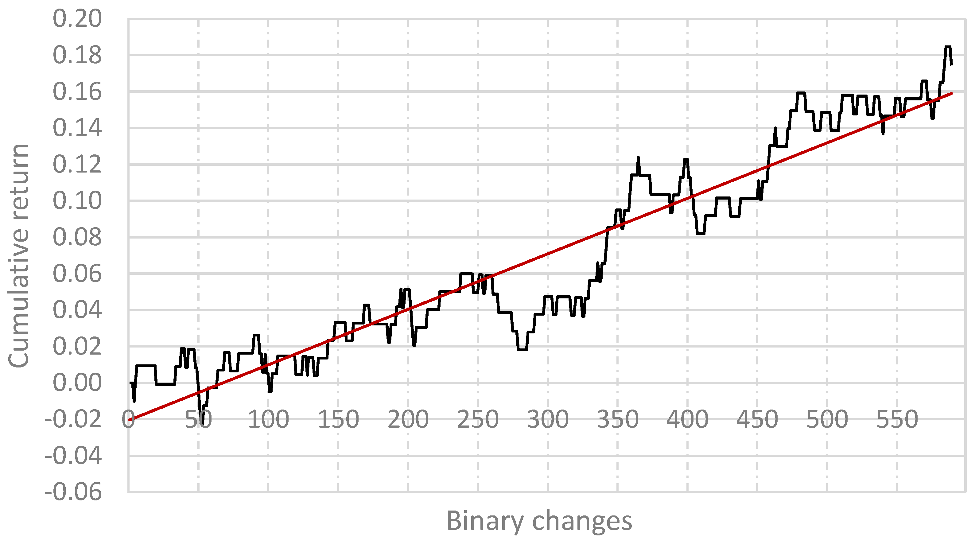
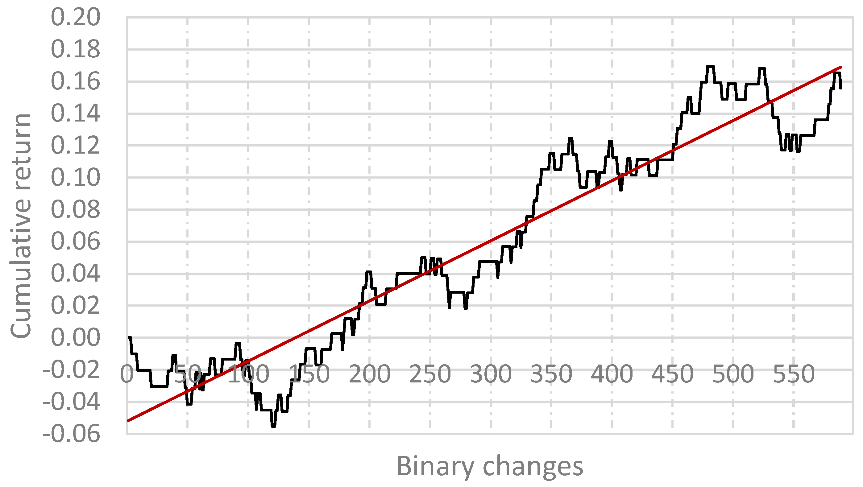
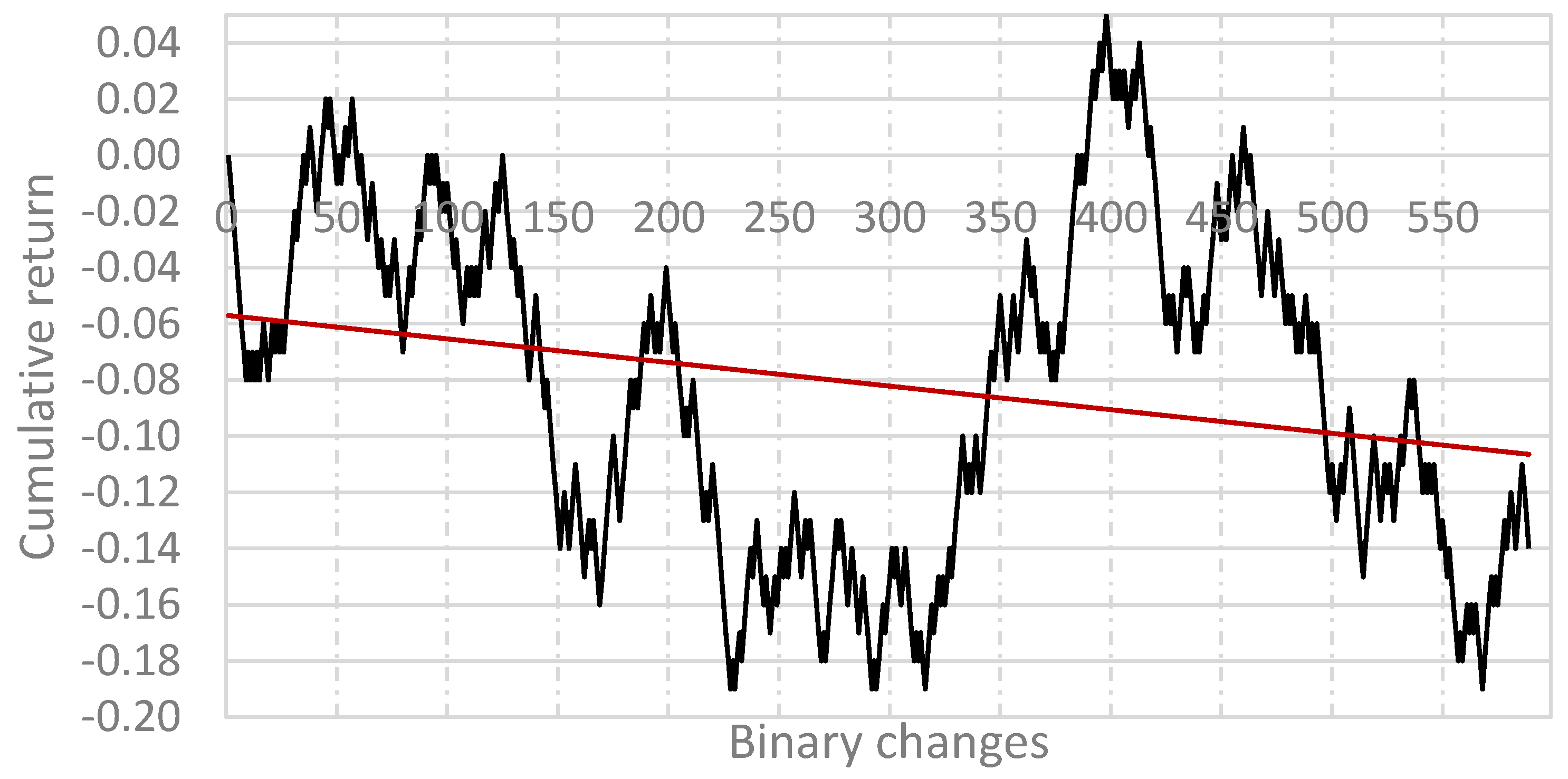
The optimization algorithm operates as follows. First, the ranges of the tested parameters are defined for each model. For each parameter combination, a prediction table is created based on the prices from the first period. Then, using the prices from the second, later period, a backtest is conducted to calculate the Calmar ratio [33]; this indicator is used to assess the effectiveness of the algorithmic trading systems [34,35]. By analyzing the backtest results, we select the parameter set for which the Calmar ratio reaches the highest value. In the final step, to verify the examined system, a backtest is conducted on the third period, covering the most recent prices.
When selecting parameters, it was assumed that the model should not exceed more than 48 states. Analyzing models with a larger number of states is not recommended due to the insufficient occurrence of many states during the testing period. In the process of selecting the optimal parameter set in the second period, systems generating fewer than 500 transactions were omitted, assuming that the system should generate at least one transaction per day during this period.
We consider the optimization process for selecting parameters for the SMBT model. Values of the parameter m in the range of 1 to 6 were verified. For all parameter sets, the Calmar ratio yielded negative values in the backtests. This result indicates that it is not possible to construct an algorithmic trading system for the oil market that offers a positive rate of return.
We will now consider a further parameter optimization process for an algorithmic trading system based on the SMBMA model. All parameter combinations within the accepted ranges were verified for δ = 100. This means that all combinations of the following parameters were analyzed: the m parameter in the range from 1 to 4 with step 1 (due to the assumed restrictions on the number of possible states), the n parameter in the range from 4 to 50 with step 1 (for n > 50, no more changes occurred) and all possible combinations of the thresholds with a 1% step for each.
The best result was achieved with the parameter set m = 3, n = 25, p = 0.05, for a decision state acceptance threshold of 0.60. During testing, 610 transactions were executed. The maximum drawdown reached 18%, and the average annual return was 7%. In the test period, the system achieved a return of 8.7%, while the maximum drawdown was only 4%, corresponding to a Calmar ratio of 2.07. The algorithmic trading system backtest for the test period is presented in Figure 3. Thus, the results from the test period fully confirmed a consistent increase in the rate of return.
Now, let us consider the optimization process for selecting parameters for an algorithmic trading system based on the SMBT model. Due to the large number of parameters, this process was divided into two stages. In the first stage, the optimal set of parameters related to trend identification ( T M , T N ) and m was selected, omitting the examination of trend thresholds. All possible combinations of parameters were verified for m in the range from 1 to 3 (due to the state limit of 48), T M in the range from 4 to 50 (for T M > 50 no more changes occurred) and T N in the range of 1 to T M / 2 .
In the second stage, based on the parameters chosen in the first one, appropriate thresholds τ , ζ were selected. The best result was obtained with the parameter set m = 3, T M = 25, T N = 2; τ = 24,000, ζ = 1, with a decision state acceptance threshold of 0.59. During testing, 746 transactions were executed. The maximum drawdown was 12%, and the average annual return reached 16%. In the test period, the system generated an 8% return rate, while the maximum drawdown was only 5%, resulting in a Calmar ratio of 1.33. The backtest of the algorithmic trading system for the test period is presented in Figure 4. The test period results demonstrated a consistent profit for the investor. Although the average annual return decreased by half, the maximum drawdown also fell by more than half, resulting in virtually identical financial efficiency in both the validation and test periods.
According to the methodology commonly applied in this type of research, e.g., [36], the obtained results can be compared to the popular “Buy and Hold” strategy. Figure 5 presents the investment results using this method during the test period from 1 January 2023 to 1 January 2024. In the examined period, this strategy was characterized by a negative Calmar ratio, indicating that its effectiveness—unlike the presented methods—does not allow for achieving a positive rate of return over a longer period.

5.4. Discussion

The results presented in this paper justify the possibility of effectively using state modelling of quotations given in a binary–temporal representation for constructing algorithmic trading systems. The developed tools are dedicated to analysts and investors, and they allow for an assessment of the probability of a given direction of a future change in the crude oil price trajectory. Also, a similar assessment can be applied in systems that fully automate the process of derivative trading, for instruments based on crude oil quotations.
Let us now consider the conclusions stemming from the optimization process of the parameter selection for each model. The best results were obtained for models SMBMA(100;3;25;0,05) and SMBT(100;3;25;2;24000;1). Both the time-weighted binary average and the trend were calculated for the last 25 changes. This kind of result indicates that this is a limiting value that influences the probability of future changes in the crude oil price trajectory. However, analyzing the long-term historical process does not lead to any improvement in the financial efficiency of the model (and even reduces it).
In the case of constructing algorithmic trading systems, the best results were obtained with the decision state acceptance threshold of 0.60 for the system built using SMBMA and 0.59 for the system using SMBT. This result shows that the decisions should be made for the states characterized by a clearly visible statistical advantage, greater or equal to 60%. Regarding the states characterized by a lower probability of success, frequent series of wrong decisions will result in a larger number of registered maximal capital dropdowns, which consequently leads to a decrease in financial efficiency.

6. Conclusions

This article presents an analysis of using the state modelling of crude oil prices in a binary–temporal representation to support investment decisions. The analysis applied all state models developed previously by authors with the binary–temporal representation, which utilizes time, averages and trend analysis. Based on these models, algorithmic trading strategies were developed and then optimized to select parameters that ensure the highest financial efficiency.
The results indicate that constructing an algorithmic trading system for the oil market with a positive rate of return is possible using the SMBMA and SMBT models—the two state models that implement known technical analysis methods, such as moving average analysis and trend analysis. In the test period, the model based on moving average analysis achieved a Calmar ratio of 2.07, while the trend model yielded a ratio of 1.33.
The results of the optimization process indicate that in crude oil price modelling in a binary–temporal representation, the influence of historical changes on the probability of the future price change direction is limited to the 25 previous changes in the price trajectory. The research findings show that in the algorithmic trading systems for the oil market, in particular, in the decision support systems constructed based on state modelling with a binary–temporal representation, the transactions should be made only for the market states for which we can calculate a probability of success of no lower than 60%. Otherwise, when some states have a statistical advantage over others, the remaining states can lead to fluctuations in the account balance (i.e., maximum dropdowns) and to the resulting decrease in the financial effectiveness of the system. The presented algorithmic trade systems with the parameters selected in this research can be implemented on an arbitrary brokerage platform, e.g., on MetaTrader with the use of MQL4 or JForex with the use of the java language, for CFD contracts on Brent crude oil.
The research results prove the high financial effectiveness of systems constructed based on models that use binary time-weighted averages and trend analysis. The limitation of the researched state models is the dependence of the results on the values of the selected parameters. Despite the fact that the test period research confirmed the proper selection of parameters, their optimal values can change in the future. Due to this, in further research, the authors want to focus on constructing adaptive models that would allow for the dynamic modification of parameters.

Author Contributions

Conceptualization: M.D.S.; methodology M.D.S.; visualization: Ż.S.; software: Ż.S., J.S. and D.W., formal analysis: M.D.S. and Ż.S., writing—review and editing, Ż.S., J.S. and D.W. All authors have read and agreed to the published version of the manuscript.

Funding

This research received no external funding.

Data Availability Statement

The original contributions presented in this study are included in this article; further inquiries can be directed to the corresponding author.

Conflicts of Interest

The authors declare no conflicts of interest.

References

  1. Kilian, L. The economic effects of energy price shocks. J. Econ. Lit. 2008, 46, 871–909. [Google Scholar] [CrossRef]
  2. van de Ven, D.J.; Fouquet, R. Historical energy price shocks and their changing effects on the economy. Energy Econ. 2017, 62, 204–216. [Google Scholar] [CrossRef]
  3. Barrera-Rey, F.; Seymour, A. The Brent Contract for Differences (CFD): A Study of an Oil Trading Instrument, Its Market and Its Influence on the Behaviour of Oil Prices; Oxford Institute for Energy Studies: Oxford, UK, 1996. [Google Scholar]
  4. Stasiak, M.D.; Staszak, Ż. Modelling and Forecasting Crude Oil Prices Using Trend Analysis in a Binary-Temporal Representation. Energies 2024, 17, 3361. [Google Scholar] [CrossRef]
  5. Tiwari, A.K.; Trabelsi, N.; Alqahtani, F.; Hammoudeh, S. Analysing systemic risk and time-frequency quantile dependence between crude oil prices and BRICS equity markets indices: A new look. Energy Econ. 2019, 83, 445–466. [Google Scholar] [CrossRef]
  6. Mensi, W.; Yousaf, I.; Vo, X.V.; Kang, S.H. Asymmetric spillover and network connectedness between gold, BRENT oil and EU subsector markets. J. Int. Financ. Mark. Inst. Money 2022, 76, 101487. [Google Scholar] [CrossRef]
  7. Salamai, A.A. Deep learning framework for predictive modelling of crude oil price for sustainable management in oil markets. Expert Syst. Appl. 2023, 211, 118658. [Google Scholar] [CrossRef]
  8. Awijen, H.; Ben Ameur, H.; Ftiti, Z.; Louhichi, W. Forecasting oil price in times of crisis: A new evidence from machine learning versus deep learning models. In Annals of Operations Research; Springer: Berlin/Heidelberg, Germany, 2023; pp. 1–24. [Google Scholar]
  9. Yin, L.; Yang, Q. Predicting the oil prices: Do technical indicators help? Energy Econ. 2016, 56, 338–350. [Google Scholar] [CrossRef]
  10. Mahdiani, M.R.; Khamehchi, E. A modified neural network model for predicting the crude oil price. Intellect. Econ. 2016, 10, 71–77. [Google Scholar] [CrossRef]
  11. Moreno, P.; Figuerola-Ferretti, I.; Muñoz, A. Forecasting Oil Prices with Non-Linear Dynamic Regression Modeling. Energies 2024, 17, 2182. [Google Scholar] [CrossRef]
  12. Weijermars, R.; Sun, Z. Regression analysis of historic oil prices: A basis for future mean reversion price scenarios. Glob. Financ. J. 2018, 35, 177–201. [Google Scholar] [CrossRef]
  13. Tudor, C.; Anghel, A. The financialization of crude oil markets and its impact on market efficiency: Evidence from the predictive ability and performance of technical trading strategies. Energies 2021, 14, 4485. [Google Scholar] [CrossRef]
  14. Degiannakis, S.; Filis, G. Forecasting oil prices: High-frequency financial data are indeed useful. Energy Econ. 2018, 76, 388–402. [Google Scholar] [CrossRef]
  15. Filippidis, M.; Filis, G.; Magkonis, G. Evaluating oil price forecasts: A meta-analysis. Energy J. 2024, 45, 49–67. [Google Scholar] [CrossRef]
  16. Kaufman, P.J. A Guide to Creating A Successful Algorithmic Trading Strategy; Wiley: Hoboken, NJ, USA, 2016. [Google Scholar]
  17. Tudor, C.; Sova, R. Flexible decision support system for algorithmic trading: Empirical application on crude oil markets. IEEE Access 2022, 10, 9628–9644. [Google Scholar] [CrossRef]
  18. Bojnourdi, E.Z.; Mansoori, A.; Jowkar, S.; Ghiasvand, M.A.; Rezaei, G.; Tabatabaei, S.A.; Keshvari, M.M. Predicting successful trading in the West Texas Intermediate crude oil cash market with machine learning nature-inspired swarm-based approaches. Front. Appl. Math. Stat. 2024, 10, 1376558. [Google Scholar] [CrossRef]
  19. Stasiak, M.D. Candlestick—The main mistake of economy research in high-frequency markets. Int. J. Financ. Stud. 2020, 8, 59. [Google Scholar] [CrossRef]
  20. Stasiak, M.D. A study on the influence of the discretisation unit on the effectiveness of modelling currency exchange rates using the binary-temporal representation. Oper. Res. Decis. 2018, 28, 57–70. [Google Scholar]
  21. Stasiak, M.D. Algoritmic Trading System Based on State Model for Moving Average in a Binary-Temporal Representation. Risks 2022, 10, 69. [Google Scholar] [CrossRef]
  22. Schwager, J.D. Getting Started in Technical Analysis; John Wiley & Sons: Hoboken, NJ, USA, 1999; Volume 19. [Google Scholar]
  23. Kirkpatrick, C.D.; Dahlquist, J.R. Technical Analysis: The Complete Resource for Financial Market Technicians; FT Press: Upper Saddle River, NJ, USA, 2010. [Google Scholar]
  24. Schlossberg, B. Technical Analysis of the Currency Market: Classic Techniques for Profiting from Market Swings and Trader Sentiment; John Wiley & Sons: Hoboken, NJ, USA, 2006. [Google Scholar]
  25. De Villiers, V. The Point and Figure Method of Anticipating Stock Price Movements Complete Theory & Practice; A Reprint of the 1933 Edition Including a Chart on the 1929 Crash; Windsor Books: New York, NY, USA, 1933. [Google Scholar]
  26. Logue, D.E.; and Sweeney, R.J. White noise in imperfect markets: The case of the franc/dollar exchange rates. J. Financ. 1977, 32, 761–768. [Google Scholar] [CrossRef]
  27. Sandubete, J.E.; Escot, L. Chaotic signals inside some tick-by-tick financial time series. Chaos Solitons Fractals 2020, 137, 109852. [Google Scholar] [CrossRef]
  28. Ghazani, M.M.; Ebrahimi, S.B. Testing the adaptive market hypothesis as an evolutionary perspective on market efficiency: Evidence from the crude oil prices. Financ. Res. Lett. 2019, 30, 60–68. [Google Scholar] [CrossRef]
  29. Okoroafor, U.C.; Leirvik, T. Time varying market efficiency in the Brent and WTI crude market. Financ. Res. Lett. 2022, 45, 102191. [Google Scholar] [CrossRef]
  30. Dimitriadou, A.; Gogas, P.; Papadimitriou, T.; Plakandaras, V. Oil market efficiency under a machine learning perspective. Forecasting 2018, 1, 157–168. [Google Scholar] [CrossRef]
  31. Stasiak, M.; Staszak, Ż. Are Changes in Crude Oil Prices Predictable? In Sustainable Global Economic Development within 2025 Vision: Research and Practice; Proceedings of the 43rd International Business Information Management Association Conference (IBIMA), Granada, Spain, 27–28 November 2024; Soliman, K.S., Ed.; IBIMA Publishing LLC: King of Prussia, PA, USA, 2024. [Google Scholar]
  32. Malkiel, B.G. Efficient market hypothesis. In Finance; Palgrave Macmillan: London, UK, 1989; pp. 127–134. [Google Scholar]
  33. Young, T.W. Calmar ratio: A smoother tool. Futures 1991, 20, 40. [Google Scholar]
  34. Psaradellis, I.; Laws, J.; Pantelous, A.A.; Sermpinis, G. Performance of technical trading rules: Evidence from the crude oil market. Eur. J. Financ. 2019, 25, 1793–1815. [Google Scholar] [CrossRef]
  35. Pardo, R. The Evaluation and Optimization of Trading Strategies; John Wiley & Sons: Hoboken, NJ, USA, 2011. [Google Scholar]
  36. Dbouk, W.; Jamali, I. Predicting daily oil prices: Linear and non-linear models. Res. Int. Bus. Financ. 2018, 46, 149–165. [Google Scholar] [CrossRef]
Figure 1. An exemplary conversion of tick quotations of the crude oil rates into a binary–temporal representation for the discretization unit of δ = 100 pips. Source: Authors.
Energies 18 00691 g001
Figure 2. General schema of a state model for a binary–temporal representation of data. Source: Authors.
Energies 18 00691 g002
Figure 3. Backtest results (with trend line) for algorithmic trading system created based on the SMBMA(100;3;25;0.05) model. Source: Authors.
Energies 18 00691 g003
Figure 4. Backtest results (with trend line) for algorithmic trading system created based on the SMBT(100;3;25;0.05) model. Source: Authors.
Energies 18 00691 g004
Figure 5. Backtest results (with trend line) for algorithmic trading system created based on ”Buy and Hold” strategy. Source: Author.
Energies 18 00691 g005
Table 1. Probability distributions for the future change direction for the SMBR (100,2) state model. Source: Authors.
StateProbab. of Inc.Probab. of Dec.Number of Occurrences
{0,0}0.49410.5059937
{0,1}0.52180.4782895
{1,0}0.48330.5167896
{1,1}0.50790.4921951
Table 2. Probability distribution for the direction of the future changes in the price trajectory for the SMBRT(100,2,3600) model. Source: Authors.
StateProbab. of Inc.Probab. of Dec.Number of Occurrences
{(0,0);0}0.49280.5072769
{(0,0);1}0.50000.5000168
{(0,1);0}0.51290.4871698
{(0,1);1}0.55330.4467197
{(1,0);0}0.47950.5205684
{(1,0);1}0.49530.5047212
{(1,1);0}0.51360.4864699
{(1,1);1}0.49200.5079252
Table 3. Probability distribution for the direction of the future changes in the price trajectory for the SMBMA(100;2;14;0.2) model. Source: Authors.
StateProbab. of Inc.Probab. of Dec.Number of Occurrences
{(0,0);1}0.52790.4721322
{(0,0);0}0.47340.5266583
{(0,0);−1}0.53120.468832
{(1,0);1}0.49290.5071495
{(1,0);0}0.56780.4322199
{(1,0);−1}0.54730.4527201
{(0,1);1}0.47590.5241477
{(0,1);0}0.52020.4798223
{(0,1);−1}0.45920.5408196
{(1,1);1}0.52340.4766321
{(1,1);0}0.37500.625048
{(1,1);−1}0.51030.4897582
Table 4. Probability distributions for the direction of future changes in the price for the states defined for the SMBT(100,2,15,3;72,000,2) model. Source: Authors.
StateProbab. of Inc.Probab. of Dec.Number of Occurrences
{(0,0);0;0}0.50450.4955111
{(0,0);0;1}0.38180.618255
{(0,0);−1;0}0.42400.5760158
{(0,0);−1;1}0.52090.4791311
{(0,0);1;0}0.52500.475040
{(0,0);1;1}0.51910.4809262
{(0,1);0;0}0.49560.5044115
{(0,1);0;1}0.49210.507963
{(0,1);−1;0}0.56920.430865
{(0,1);−1;1}0.50840.4916297
{(0,1);1;0}0.64790.352171
{(0,1);1;1}0.51060.4894284
{(1,0);0;0}0.45190.5481104
{(1,0);0;1}0.50770.492365
{(1,0);−1;0}0.51250.487580
{(1,0);−1;1}0.50690.4931288
{(1,0);1;0}0.36510.634963
{(1,0);1;1}0.48310.5169296
{(1,1);0;0}0.62390.3761117
{(1,1);0;1}0.38590.614157
{(1,1);−1;0}0.43900.560941
{(1,1);−1;1}0.50760.4924262
{(1,1);1;0}0.45190.5481135
{(1,1);1;1}0.51910.4808339
Table 5. Prediction table for the SMBMA(100,2,14,0.2) with an assumed threshold of 0.52. Source: Author.
StateRecommendationProbab. of Success
{(0,0);1}BUY0.5279
{(0,0);0}SELL0.5266
{(0,0);−1}BUY0.5312
{(1,0);1} 0.5071
{(1,0);0}BUY0.5678
{(1,0);−1}BUY0.5473
{(0,1);1}SELL0.5241
{(0,1);0}BUY0.5202
{(0,1);−1}SELL0.5408
{(1,1);1}BUY0.5234
{(1,1);0}SELL0.6250
{(1,1);−1} 0.5103
Disclaimer/Publisher’s Note: The statements, opinions and data contained in all publications are solely those of the individual author(s) and contributor(s) and not of MDPI and/or the editor(s). MDPI and/or the editor(s) disclaim responsibility for any injury to people or property resulting from any ideas, methods, instructions or products referred to in the content.

