Short-Term Building Electrical Load Prediction by Peak Data Clustering and Transfer Learning Strategy

Abstract

With the gradual penetration of new energy generation and storage to the building side, the short-term prediction of building power demand plays an increasingly important role in peak demand response and energy supply/demand balance. The low occurring frequency of peak electrical loads in buildings leads to insufficient data sampling for model training, which is currently an important factor affecting the performance of short-term electrical load prediction. To address this issue, by using peak data clustering and knowledge transfer from similar buildings, a short-term electrical load forecasting method is proposed. First, a building’s electrical peak loads are clustered through peak/valley data analysis and K-nearest neighbors categorization method, thereby addressing the challenge of data clustering in data-sparse scenarios. Second, for peak/valley data clusters, an instance-based transfer learning (IBTL) strategy is used to transfer similar data from multi-source domains to enhance the target prediction’s accuracy. During the process, a two-stage similar data selection strategy is applied based on Wasserstein distance and locality sensitive hashing. An IBTL strategy, iTrAdaboost-Elman, is designed to construct the predictive model. The performance of proposed method is validated on a public dataset. Results show that the data clustering and transfer learning method reduces the error by 49.22% (MAE) compared to the Elman model. Compared to the same transfer learning model without data clustering, the proposed approach also achieves higher prediction accuracy (1.96% vs. 2.63%, MAPE). The proposed method is also applied to forecast hourly/daily power demands of two real campus buildings in the USA and China, respectively. The effects of data clustering and knowledge transfer are both analyzed and compared in detail.

1. Introduction

In recent years, along with the increased building electrification, the proportion of electricity used in buildings has grown rapidly. In building-intensive cities such as Hong Kong and Shanghai in China, the proportion of building electricity consumption in total social electricity consumption has exceeded 90% [1]. With the gradual penetration of new energy generation and storage to the building side, the fluctuation and randomness of power generation/consumption also brought new challenges to the stability and optimal operation of the power grid. Accurately predicting a building’s short-term electricity consumption plays an increasingly important role in peak demand response and energy supply/demand balance. For load prediction tasks with plenty of historical data, data-driven approaches are believed to be more convenient and accurate than mechanism models. Various types of machine learning and deep learning models have been widely used in the field of building energy prediction [2,3,4]. The related research continues to make progress with respect to data analysis [5,6], model construction [7,8], and algorithm design [9]. However, when buildings lack sufficient high-quality historic data, or the sampled data distribution is unbalanced, traditional data-driven models no longer guarantee prediction accuracy. In the face of such data scarcity or imbalance problems, transfer learning of knowledge is an important direction.

1.1. Related Work

Transfer learning utilizes knowledge from source domain(s) to assist in accomplishing the target task. This approach relaxes two basic requirements of the data-driven models: the distributions of the training and testing sets could be different; the model could guarantee high performance even if the available training data from target domain are limited. The primary mission in transfer learning is to identify source domain data similar to the target domain, which are suitable for auxiliary training of target model. Currently, there are various similarity judgment methods, and the commonly used ones include maximum mean discrepancy (MMD) [10], Wasserstein distance (WD) [11], and maximal information coefficient (MIC) [12]. MMD maps the original variables to the reproducing kernel Hilbert space (RKHS) [13] and then calculates the distance between the two distributions to determine the similarity. Li et al. [14] selected two educational buildings with the highest similarity from more than 1000 buildings by using MMD and performed load prediction through transfer learning. If the single source domain and the target domain do not overlap at all or the overlap is very small, the WD method is more appropriate for similarity judgment [11]. In addition, by measuring the correlation between samples from different distributions (MIC method), the data similarity could also be determined [12]. Lu et al. [15] measured the similarity of time series data from the target and source domains by introducing the MIC method and used transfer learning to improve the accuracy of load prediction with scarce historical data. Wei et al. [16] combined WD and MIC methods to find the source domain with high similarity, and knowledge was transferred to improve the accuracy and robustness of the target predictive model. Similar studies are also reported in the literature [17,18].

From the perspective of transfer models, the currently used models mainly belong to model-based transfer learning (MBTL). The common practice is: pre-training the learning model using building datasets from similar regions or types (schools, residences, etc.), then fine-tuning parameters of the pre-trained model with small amounts of target-domain data to improve the prediction accuracy. For example, Li et al. [19] interpolated the missing data from the target sensor using bidirectional LSTM and transfer learning, which improved the robustness and prediction accuracy. Gao et al. [20] proposed a transfer learning-based multilayer perceptron (TL-MLP) to improve the prediction performance of buildings without sufficient labeled data. Similar studies can be found in [21,22,23]. Pinto et al. [24] summarized most of the current transfer learning strategies for building energy prediction. In the survey, 57 of the 77 papers on transfer learning used the MBTL method. However, when the training data are relatively sparse in the target domain, the instance-based transfer learning (IBTL) is more effective, because IBTL is able to select suitable samples directly from the source domain and assigns weights to the samples according to the prediction errors, which would help obtain training data of higher quality. Zeng et al. [25] integrated the advantages of weighted support vector regression (WSVR) and transfer learning based on TrAdaboost to improve the prediction accuracy. Li et al. [26] compared methods such as MBTL and IBTL in predicting the cross-building energy consumption of office buildings and academic buildings. Results showed that the IBTL strategy was more stable. Similarly, Li et al. [27] found by comparison that instance-based boosting-type transfer learning methods were able to obtain more complete features of the target domain data, thus could further improve the prediction accuracy.

When the data distribution between single source and target domain differ significantly, similar data searching could expand to multiple source domains [28]. Lu et al. [29] introduced a multi-source IBTL building load prediction combining LSTM and multi kernel MMD domain adaptation. It is noted that as the number of source domains increases, so does the amount of redundant data. In 2024, Li et al. [30] investigated the impact of the quantity of source domain buildings on prediction accuracy of IBTL.

Table 1. Related papers on building energy prediction using IBTL method, since 2022.

Literature	Source Domain	Similarity Judgment Method	Predictive Model	Building Type
Li et al. (2022) [26]	Single source	MMD	DANN-LSTM	Office/Education
Li et al. (2022) [14]	Single source	MMD	iTrAdaboost-BP	Education
Lu et al. (2022) [15]	Single source	MIC	LSTM	Residence
Yuan et al. (2023) [17]	Single source	MMD	Attention-CNN-LSTM	Commerce
Lu et al. (2023) [29]	Multi-source	DTW	MK-MMD-LSTM	Railway building
Qian et al. (2024) [31]	Multi-source	DTW	iTrAdaboost-LSTM	Office/Education
Li et al. (2024) [30]	Multi-source	WD	NNS-iTrAdaboost-LSTM	Education

summarizes the researches on IBTL based building energy prediction in the last three years. The source domain number, similarity judgment method, and predicted time scale are all listed.

According to the literature review on transfer learning, the current models mainly treat target domain datasets as a whole. However, for the short-term building electrical load prediction, the main error actually comes from the error of peak loads’ prediction. The sampled data during the peak times are relatively insufficient due to their low occurring frequency, even though the data in other periods may be redundant. These inherent data distribution’s imbalance particularly affects the performance of short-term load prediction. To this end, peak data’s recognition and IBTL based transfer learning may be a more targeted and efficient prediction method. The classification of peak data from target domain needs an available data clustering method. The unsupervised K-means or fuzzy C-mean clustering (FCM) methods could be used for such clustered prediction problems [32,33]. However, such data clustering requires sufficient labeled data to identify the intrinsic pattern, which are not available in data-sparse scenarios. A proper data clustering approach is still needed for peak loads classification. Based on this, a more efficient transfer learning strategy for short-term building electrical load prediction is explored in this study.

1.2. Main Contribution of This Work

To address the above issues, using peak data clustering and knowledge transfer from similar buildings, a building’s short-term electrical load forecasting method based on clustered transfer learning strategy is proposed. The main contributions of this paper include:

(1) By analyzing the error source of short-term building electrical load prediction, the historical peak load data are clustered according to timestamp and extreme search. Based on the obtained data clusters, the supervised KNN algorithm is then used for testing data classification. Addressing the scarcity of clustered peak data, a transfer learning strategy is designed to enhance the training procedure so as to improve the whole prediction accuracy.

(2) A multi-source instance-based transfer learning strategy is designed. The Wasserstein distance is used to filter multiple buildings similar to the target one as the source domains, from which the most helpful data samples are further selected by locality sensitive hashing (LSH) for auxiliary model training. An improved TrAdaboost (iTrAdaboost) algorithm is combined with Elman networks for a transfer learning type’s model construction.

(3) Three different case studies are carried out for performance validation. A benchmark dataset from ASHRAE is used to verify and compare the accuracy of the proposed model with other methods. On this basis, two campus buildings in the USA and China are selected as practical cases to further verify the performance at the respective different predictive time scales (hourly and daily) and knowledge transfer scopes.

1.3. Paper Organization

The second section describes the framework of transfer learning and the related data clustering method. In the third section, the proposed model is applied to perform load prediction on the public dataset and two actual buildings, respectively. The results are analyzed in detail. The last section gives a brief conclusion.

2. Principles and Methods

2.1. Instance-Based Transfer Learning

IBTL reuses labeled data from source domains to help train a model for the target task more accurately. Because there are differences between target and source domains, data samples from source domains do not necessarily improve the model performance [34]. An effective boosting-style approach involves adjusting the weights of source domain instances based on prediction errors, identifying misleading data, and iteratively training the target domain model, which leads to better results for the trained classifiers/predictors.

One of the boosting style methods, TrAdaboost [35], is chosen in this study. By increasing the weights of the samples that are favorable to the target task and decreasing the weights that are unfavorable to the target task, the model accuracy is improved [35]. The original TrAdaboost is used for classification, but building load prediction is considered a regression problem. Appropriate modifications are made on the basis of original TrAdaboost algorithm, which include:

(1) The weight update parameter of traditional TrAdaboost is

$${\beta }_t={\displaystyle \frac{{\epsilon }_t}{1-{\epsilon }_t}}.$$

(1)

For binary classification, the error rate ${\epsilon }_t$ of the original TrAdaBoost algorithm is less than 0.5. In the improved TrAdaBoost algorithm, when the error rate is greater than 0.5, it is reset to 0.5, which ensures the stability and effectiveness of the algorithm for forecasting tasks.

(2) The threshold ($\gamma$) of TrAdaboost is fixed for the classification problem. In regression prediction, it is updated by a function

$$\Delta {\gamma }_t=-\eta {\displaystyle \frac{\partial E_t}{\partial y_t}}.$$

(2)

Thus, the threshold $\gamma$ will be dynamically changed according to the prediction error rate.

The Elman Network [36] is chosen as the sub-learners in the iTrAdaboost algorithm. This is because a building energy system usually has complex nonlinear relationships, which is what the Elman model is good at capturing. At the same time, the Elman model has the advantages of a simple structure, computational efficiency, and consideration of temporal information. Details of the transfer learning model (called iTrAdaboost-Elman) are given in Figure 1, where ${\omega }_N$ is the initial weight vector of the training set, and $h_N$ is the base prediction in the target domain. The expressions x and y are the input features and energy consumption values of the training set, respectively; n and m are the number of data samples from source and target domain, respectively.

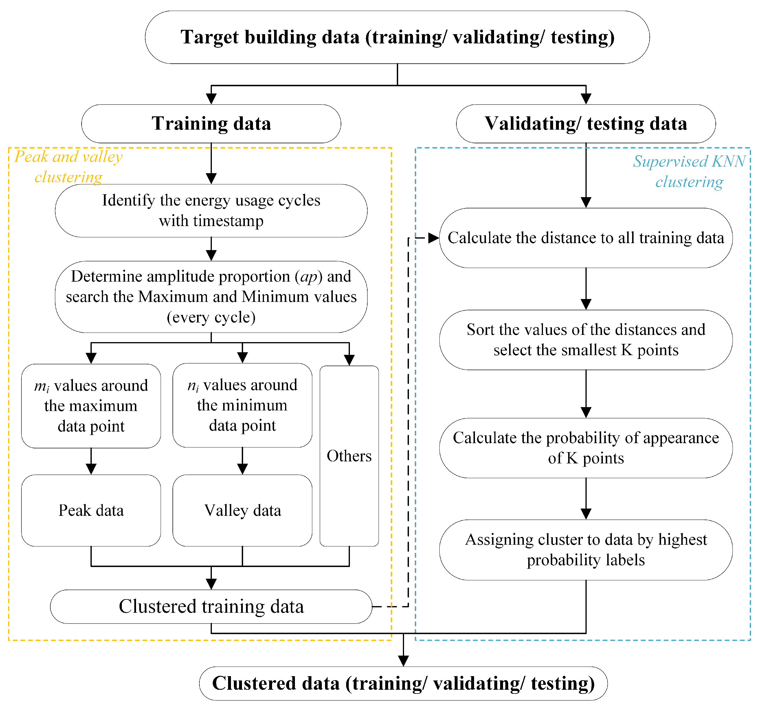
2.2. Data Clustering Method

By analyzing the error source of short-term building electrical load prediction, the errors from peak loads seriously affect the whole prediction performance. Data clustering helps in finding the underlying patterns and characteristics within data samples, and it plays a key role in prediction and analysis tasks. As reviewed in the Introduction, various data clustering methods (such as K-means and FCM) have been applied for building energy clustering and prediction. However, data’s transfer learning task in a data scarcity scenario naturally prevents the application of such traditional clustering methods, because the required sufficient labeled data can hardly be obtained.

To identify peak loads in limited historical data, the timestamp and extreme search method is used in this study. First, the dataset combined with timestamp is sorted by time series and the energy usage cycle is identified (24 hours a day, 7 days each week, etc.). In every energy usage cycle, the extreme values (maximum/minimum) are searched as peak and valley points. Then, based on the amplitude of each energy usage cycle (the difference between the maximum and minimum loads), a amplitude proportion ap (say, 15%) is determined to classify peak and valley data clusters. In this way, $m_i$ data samples around the peak point are clustered as the peak data, and $n_i$ data samples around the valley point are clustered as the valley data. The rest of the data are clustered as the others. The specific values of $m_i$ and $n_i$ are depended on the proportion ap.

It should be pointed out that only historical data can be clustered using the above method. For unknown data of the future (as validation/testing sets), such extreme searching is not feasible. We classify datasets for validation/testing according to the distances to the obtained three clusters (peak/valley/others). The K-nearest neighbors (KNN) [37] is utilized, and by setting key parameter K, the nearest data points are clustered. The specific flowchart of the data clustering is shown in Figure 2.

2.3. Two-Stage Selection of Similarity Data

This study uses a two-stage method for similar data selection from source domains. First, multiple source domain buildings are selected based on WD. Then, the LSH method is introduced to select similar data from them, so as to reduce the impact of redundant data in the source domain dataset on transfer learning.

2.3.1. Similar Buildings Recognition

By measuring the distance between two distributions, the similarity between them can be determined. For the commonly used MMD method, when two distributions (buildings) do not overlap or overlap very little, the results will be close to zero or do not reflect the true distance of the distributions. In contrast, WD directly calculates the minimum cost of converting one distribution to another, which could reflect the similarity more effectively. The Wasserstein distance can be defined as

$$W_p(\mu ,\nu )={\left(\underset{\pi \in \Gamma (\mu ,\nu )}{inf}{\int d(m,n)}^{p}d\pi (m,n)\right)}^{1/p},$$

(3)

where $d(m,n)$ denotes the distance between points m and n, e.g., the Euclidean distance; $\Gamma (\mu ,\nu )$ is the set of all joint probability distributions whose marginals are distributed as $\mu$ and $\nu$; p is the order between $\mu$ and $\nu$. More details can be found in [11]. By calculating the WDs, similar source domain buildings are selected.

Further, an optimal indicator is set for determining the number of source domains [38]. Considering optimal prediction accuracy and a small number of source domains, the function is defined as

$$\underset{p}{min}f\left(p\right)=\lambda \times {\displaystyle \frac{p}{q}}+(1-\lambda )\times MAPE(p,q)$$

(4)

where p and q are the amount of selected source buildings and candidate source buildings, respectively. The $MAPE(p,q)$ is the error of the predictive model using p source domains to predict and obtain the model parameters; $\lambda$ is the weighting coefficient to balance the two terms. In practice, it is difficult to find the exact $\lambda$. For this study, the $\lambda$ is roughly adjusted to 0.8 according to expert experience. The optimal number of source domains p is determined through these two steps: First, minimize the number of source domains to reduce computational load while ensuring model performance; then, select as many source domains as possible to enhance model performance.

2.3.2. Similar Data Selection

In the field of electric load prediction, nearest neighbor search (NNS) has been used to find similar data from source domain buildings [30]. Different from NNS, LSH achieves approximate nearest neighbor search (ANNS) [39] by mapping high-dimensional data points to a low-dimensional hash space such that similar data points have a high probability of being mapped to the same hash bucket [40]. LSH is able to efficiently perform ANNS in high-dimensional spaces and usually has faster speed and smaller storage requirements than NNS, making it more suitable for finding similar high-dimensional data from source domains.

The specific searching procedure is as follows:

S1. Map the data to a lower dimensional space to reduce computational complexity and the impact of dimensionality curse.

S2. By constructing a hash table through one or more hash functions, similar data points have a higher probability of being mapped into the same hash bucket. The Minhash function is chosen in this study.

S3. Map data points into corresponding hash buckets according to the chosen hash function. Each hash bucket contains a set of similar data points, possibly the most neighboring ones.

S4. According to the query data points, by using the same hash function, the query points are mapped to the corresponding hash buckets, then the set of nearest neighbor candidate points are searched from the hash buckets.

S5. The set of candidate points is further filtered and sorted to identify the nearest neighbor data points. Euclidean distance, cosine similarity, or other similarity measurements are generally used to calculate and rank the closest neighboring points. The Euclidean distance is chosen for this study.

The primary used parameters are the similarity threshold $\sigma$ (0 to 1) and the number of hash functions $\eta$. A higher $\sigma$ results in selecting fewer similar data points. For this study, $\sigma$ is set to 0.4, meaning only data with the similarity of 0.4 or greater will be selected. The larger the number of hash functions $\eta$, the more accurate the estimated similarity. But it also requires calculating and storing more hash values, which will increase the computation time to some extent. For this study, the value of $\eta$ is set to 128.

2.4. The Proposed Predictive Model Framework

In this study, data clustering is combined with knowledge transfer learning for efficient short-term building electrical load prediction. The overall procedure of the prediction framework includes three parts.

First, data clustering is performed to pick out building’s peak/valley loads. Concretely, building’s historical electrical loads are clustered into three categories (peak/valley/others) through energy usage cycle identification and extreme value searching. Then, based on the recognized data clusters, the data from validating and testing sets are classified by KNN method. Second, similar data from source domains are selected for transfer learning by a two-stage method. Specifically, the similar buildings are selected by calculating the WD metric; then, by the LSH method, most helpful data samples from the above similar buildings are picked to construct an auxiliary dataset for transfer learning. It is noted that only peak/valley data from source domains are identified and picked by this two-stage method. Third, the Elman network is constructed and iteratively trained as sub-learners with the proposed iTrAdaboost algorithm. The transfer learning procedure is carried out only for the peak/valley data that are insufficient for model training. For the data cluster of “others”, the Elman model is directly used for prediction. In the following section, three case studies investigate the performance of the proposed method. Figure 3 summarizes the overall structure of this study.

3. Case Studies

In this section, the performance of proposed method is first validated on a public dataset. Then, hourly/daily power loads from two real campus buildings in the USA and China will be used for prediction experiments. To objectively assess the performance, three commonly used indicators—mean absolute error (MAE), mean absolute percentage error (MAPE), and root mean square error (RMSE)—are calculated for this study. The mathematical formulas are provided as follows:

$$\mathrm{MAE}={\displaystyle \frac{{\sum }_{i=1}^n\left|Y_i-{\widehat{Y}}_i\right|}{n}},$$

(5)

$$\mathrm{MAPE}={\displaystyle \frac{1}{n}}\sum _{i=1}^n{\displaystyle \frac{\left|Y_i-{\widehat{Y}}_i\right|}{Y_i}},$$

(6)

$$\mathrm{RMSE}=\sqrt{{\displaystyle \frac{{\sum }_{i=1}^n{(Y_i-{\widehat{Y}}_i)}^2}{n}}},$$

(7)

where n is the data amount, $Y_i$ is the measured data value, and ${\widehat{Y}}_i$ is the predicted data value.

All calculations in this study were completed in MATLAB-R2023b software (Intel(R) Xeon(R) Gold 5222 CPU, 3.80 GHz, and 32 GB RAM). All figures and tables were output and sorted out by MATLAB software. Data processing methods and some parameters are set according to Section 2.

3.1. Benchmark Case

The dataset of this benchmark case is derived from the Great Energy Predictor III competition organized by ASHRAE [41]. The performance validation and model comparison are based on this case because of its good data integrity and openness.

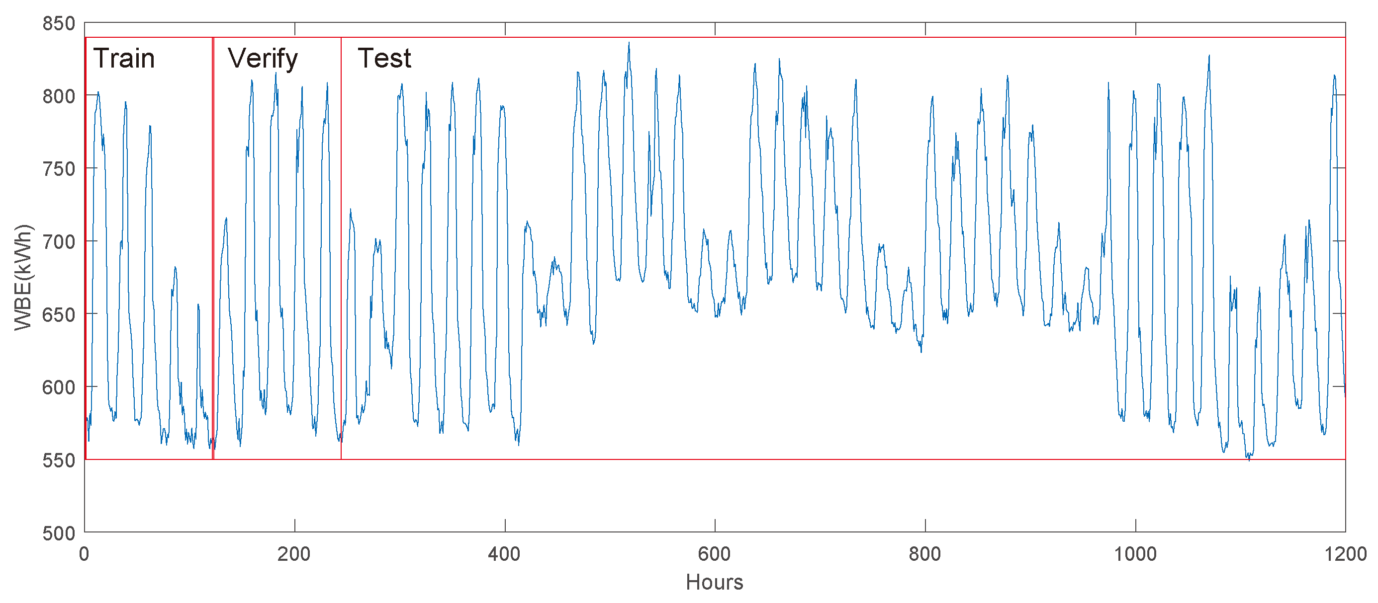
3.1.1. Description of Target and Source Domain Buildings

(1) Target domain building

In the public dataset, we randomly select an academic building as the target building. The basic information about the building is provided in

Table 2. Relevant information of similar buildings (sorted by WD), benchmark case.

Building No.	WD	Building Type	Square Feet	Air Temperature (°C)	Sea Level Pressure
Target	-	Education	182,943	0–38.3	987.3 –1035.9
S1(#1092)	1006.48	Office	105,167	−26.1–37.8	987.2–1046.5
S2(#1289)	1009.99	Education	194,441	−17.2–35.6	982.6–1043.4
S3(#780)	1011.23	Education	120,836	−16.1–36.7	986.8–1042.7
S4(#192)	1011.57	Education	151,637	2.2–48.3	996.1–1032.2
S5(#1328)	1014.73	Education	279,840	−28.8–11.8	983.6–1036.6
S1447(#803)	5093.44	Education	182,986	−28.8–33.9	983.6–1043.8
S1448(#794)	5151.56	Education	731,945	−28.8–33.9	983.6–1043.8
S1449(#801)	5326.67	Education	484,376	−28.8–33.9	983.6–1043.8

. The original features related to the energy usage include: air temperature ($T_{-}air$), sea level pressure ($S_{-}p$), time sine (sh), time cosine (ch), dew temperature ($T_{-}dew$), holiday flag ($H_{-}flag$), previous hourly loads ($y-1$), and previous two-hourly loads ($y-2$).

Correlation analysis is employed to screen the key features, and those with low correlation to the actual energy consumption values are removed. Figure 4 shows the Pearson correlation coefficient results, where WBE is the whole building electricity load. After feature selection, $S_{-}p$ and sh are eliminated and the other six features are retained.

A total of 1200 sets of hourly data since January 2016 are chosen for model construction. The dataset is divided into three parts (training, validation, and testing) with the ratio of 1:1:8. To simulate the data scarcity scenario, only the first 120 hours’ data are for model training, and the remaining 1080 hours’ data are for model validation and performance testing. The time series of the target building’s energy loads and corresponding data division are shown in Figure 5.

(2) Source domain buildings

For this case study, the remaining 1000+ buildings in the public dataset form a candidate building pool for similar building selection. By calculating the WD value between each building in the candidate pool and the target building (only using training data), four buildings with the highest degrees of similarity (minimum WDs) are finally picked out (denoted as S1, S2, S3, and S4). Calculating the WD value between buildings in the public dataset, which has a storage size of about 1 GB, typically takes no more than half an hour. Table 2 lists the relevant information of similar buildings sorted by WD.

3.1.2. Data Clustering of Target Domain

Since hourly data have a strong 24-hour periodicity, a moving average filtering process on the training set is performed to prevent probable outliers from affecting the judgment of peak loads. Then, based on the data clustering method mentioned in Section 2.2, the training data from target domain is divided into three clusters: “peak”, “valley”, and “others”. The amplitude proportion is set to 15%. The clustered result on the training set from the target domain is shown in Figure 6. The validating and testing sets are classified using KNN method based on the clustered features. The KNN classification is based on the procedure described in Section 2.2.

3.1.3. Data Selection from Similar Buildings

To enhance the target prediction’s accuracy, only peak/valley clusters containing insufficient samples are supplemented with data from the source domains. The IBTL algorithm is carried out for these two clusters’ prediction. From four similar buildings selected by the WD metric, similar data are chosen by the LSH method. A total of 523 sets of hourly data from these four source domains is retained and used for knowledge transfer learning. To show the high dimensional features more directly, the t-SNE algorithm is used to reduce the feature dimension, and the effect of similar data selection by LSH is shown in Figure 7.

3.1.4. Prediction Results

Base on the prediction strategy presented above, 120 hours’ training data are clustered into three categories. Among them, “peak/valley” clusters carry out the proposed instance-based transfer learning model (iTrAdaboost-Elman). Considering that the “others” cluster has a strong cyclical trend, the data of this cluster are supplemented with Gaussian noise instead of knowledge transfer from a similar building, and the Elman network is used for this cluster’s load prediction.

For performance investigation, 80% of the total data (960 hours’ data) are used for model testing. The predicted loads are recorded in Figure 8. The fitted scatter validation results are recorded in Figure 9. Quantitative results show that, with only 120 hours’ training data, the MAE of the proposed model reaches 13.68 kWh (MAPE: 1.96%, RMSE: 19.31 kWh). The basic data-driven model Elman network and transfer learning iTrAdaboost-Elman model are also realized without data clustering. Compared with these two models, the MAE of the proposed model is reduced by 49.2% (Elman) and 25.6% (iTrAdaboost-Elman), respectively. The detailed results of the three models are all recorded in

Table 3. Performance comparison with proposed model and Elman/iTrAdaboost-Elman, benchmark case.

Model	Transfer Learning	Data Clustering	MAE (kWh)	MAPE (%)	RMSE (kWh)
Elman	No	No	26.94	3.80	35.17
iTrAdaboost-Elman	Yes	No	18.39	2.63	24.31
Proposed model	Yes	Yes	13.68	1.96	19.31

.

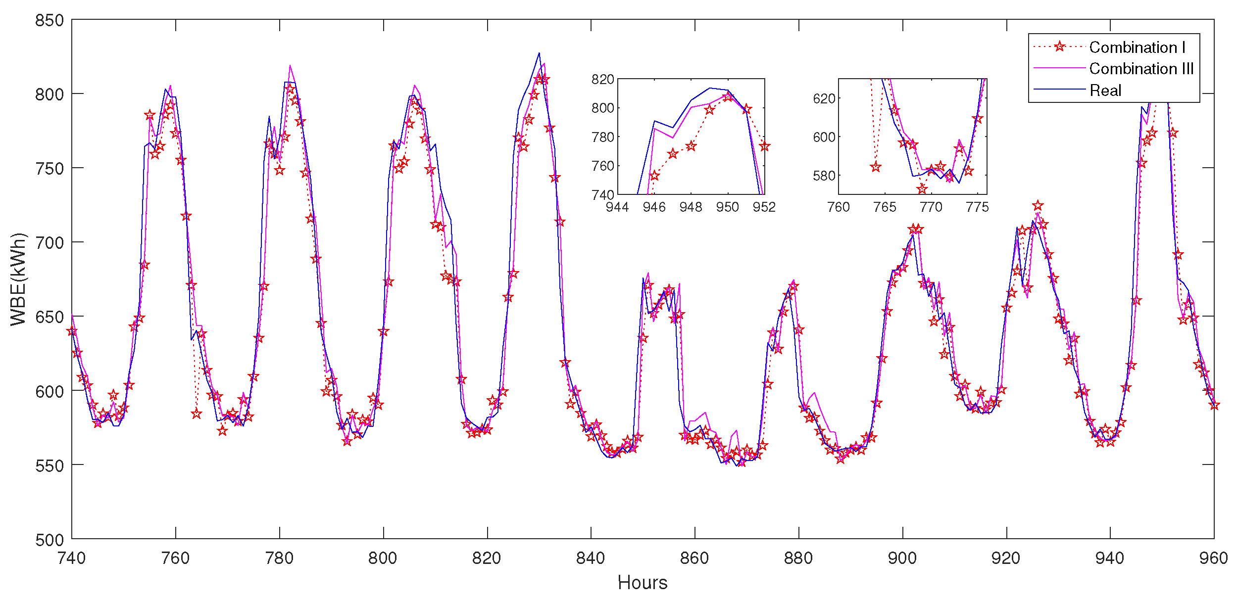
3.1.5. Discussion and Analysis

To investigate the performance of the proposed model, a brief discussion is presented for the following four aspects:

(1)

The combination effect of data clustering and transfer learning

To compare the combination effect, three different combinations of data clustering and transfer learning strategy are carried out as follows: (I) Transfer learning strategy (iTrAdaboost-Elman) is applied on all data without clustering; (II) Transfer learning strategy is applied on all data after data clustering; (III) Transfer learning strategy is only applied on clusters of “Peak”/“Valley”. The cluster of “Others” with a strong cyclical trend does not use training data from other buildings, and the traditional Elman model is applied. To show the effect of LSH data selection, the above three compared models do not use LSH-based similar data selection, and all data from similar buildings constitute the entire source domain dataset. The prediction results are compared with that of proposed model with LSH.

Results are all recorded in Figure 10 and

Table 4. Prediction results for three combinations of data clustering and transfer learning (MAPE, %), benchmark case.

Transfer Learning	Data Clustering	LSH	“Peak” Data	“Valley” Data	“Others” Data	Integrated
I. All data	No	No	2.22	1.59	3.40	2.63
II. All clusters	Yes	No	2.10	1.43	3.26	2.50
III. Clusters of Peak/Valley	Yes	No	2.10	1.43	2.29	2.05
Proposed model	Yes	Yes	1.91	1.30	2.29	1.96

. It is seen that: (1) Comparing results from Combination II and I, data clustering could enhance the transfer learning effect, and the whole prediction accuracy is improved (2.63 vs. 2.50, MAPE); (2) Comparing results from Combination III and II, the transfer learning strategy for peak/valley data is a more targeted and efficient prediction method, and the prediction accuracy is further improved to 2.05 (MAPE); (3) Comparing results from Combination III and I, the peak data after clustering (without LSH) can be better predicted (2.63 vs. 2.05, MAPE); (4) Using LSH-based similar data selection, the proposed model achieves the best prediction accuracy: 1.96 (MAPE).

(2)

The influence of KNN classification on the overall prediction accuracy

As we have mentioned, the realtime sampled data for model testing could not be clustered by the same method as historical data for training. The KNN method is used for these data, which would inevitably introduce the classification error to some extent. To analyze the influence of KNN classification on the overall prediction accuracy, three different values of KNN key parameter K are set, and their classification results are compared with that of the timestamp/extreme search method. Results are recorded in

Table 5. Comparison of KNN classifications on the overall prediction accuracy, benchmark case.

Classification	Classification	Amounts of	Prediction Accuracy (MAPE, %)
Method	Accuracy (%)	Clustered Data	“Peak”	“Valley”	“Others”	Overall
Timestamp	100.0	226/243/491	1.63	1.13	2.50	1.95
KNN (K = 4)	71.9	349/172/439	2.02	1.40	2.34	2.06
KNN (K = 5)	74.2	317/198/445	1.96	1.30	2.29	1.96
KNN (K = 6)	72.8	347/181/432	2.02	1.37	2.32	2.03

. It is seen that, supposing the testing data is sampled real-time in practice, the KNN method will result in a classification error around 27%. The prediction accuracy for peak/valley clusters tend to decrease compared with that of timestamp/extreme search method, but the impact on the overall prediction accuracy is not significant. When K is set to 5, the prediction accuracy achieves the best score (1.96%, MAPE), which is almost the same as that of timestamp classification (1.95%).

(3)

The influence of LSH data selection on the overall prediction accuracy

As Table 4 shows, the LSH similar data selection could enhance transfer learning-based prediction accuracy. The value of similarity threshold $\sigma$ in LSH determines the amount of selected data for “Peak” and “Valley” source domains’ construction, and its influence on the prediction accuracy is investigated here. Four feasible values of similarity threshold $\sigma$ are set in LSH, and other model parameters remained consistent. The prediction results are compared in

Table 6. Comparison of different similarity threshold $\sigma$ on overall prediction accuracy, benchmark case.

LSH Usage	Value of Threshold ($\mathit{\sigma }$)	Amount of Selected Data	MAE (kWh)	MAPE (%)	RMSE (kWh)	Time (s)
No	−	−	18.39	2.63	24.31	79.5
Yes	0.30	2024	14.00	2.01	19.48	120.9
Yes	0.35	1701	14.10	2.02	19.50	110.5
Yes	0.40	523	13.68	1.96	19.31	87.0
Yes	0.45	183	14.30	2.06	19.65	82.7

. As the similarity threshold changes from 0.3 to 0.45, the amount of selected data gradually decreases from 2024 to 183, and the calculation time also decreases accordingly from 120.9 s to 82.7 s (10 times average). The prediction accuracy does not exhibit a similar monotonic decrease. When $\sigma$ is set to 0.4, 523 sets of similar data are selected and the predictive model achieves optimal accuracy (1.96%, MAPE).

(4)

Performance comparison with other reported models

Through the benchmark dataset, the previously reported data-driven models, including BP [42], ELM [43], RF [44], RBF [45], and LSTM [46], are also constructed for performance comparison. The parameter setting is consistent with the references. The average results of twenty runs per model are recorded in

Table 7. Performance comparison between the proposed model and the previous models, benchmark case.

Model	MAE (kWh)	MAPE (%)	RMSE (kWh)	Time (s)
Elman	26.94	3.80	35.17	1.72
BP [42]	32.11	4.71	40.70	1.25
ELM [43]	34.30	5.01	45.07	1.13
RF [44]	27.64	4.03	35.13	1.17
RBF [45]	27.39	3.97	37.51	19.12
LSTM [46]	32.13	4.68	40.43	16.78
MMD-iTrAdaboost-BP [14]	18.83	2.71	25.05	79.5
NNS-iTrAdaboost-LSTM [30]	17.81	2.56	23.00	436.7
Proposed model	13.68	1.96	19.31	87.0

. Compared with these traditional data-driven models, the Elman model achieves the best prediction performance on the dataset, which is the reason why Elman is chosen as the sub-learners in the proposed transfer learning strategy.

Further, two previously reported transfer learning methods without data clustering are built according to the literature [14,30]. The model parameters are consistent with those in the literature, and the average results of twenty runs per model are recorded. The results are compared with the proposed strategy in Table 7. It is seen the proposed model reaches the best accuracy (1.96%, MAPE). From the respective of model complexity and time consumption, although the transfer learning models consume more time than traditional models, the prediction time of the proposed model is less than 100 s, which is acceptable for hourly load prediction.

3.2. Campus Building Case A

3.2.1. Description of Target Building Data

To verify the adaptivity and robustness of the model, a real campus building from University of Wyoming, USA, is selected. It has three floors, about 6000 square meters in total. Only 1200 hourly data from September to October, 2017 are picked from the Information Technology Center Building. All weather and power load data come from local sensing/metering devices. The data division for training/validating/testing is consistent with that of benchmark case (1:1:8), i.e., only the first 120 hours’ data are considered as known historical data for training. Figure 11 shows the outside of the target building.

For the target building, the original data features include eight variables: outdoor dry-bulb temperature (T), the previous hourly temperature ($T-1$), the previous two hours ($T-2$), holiday-flag, time-sine (sh), time-cosine (ch), the energy consumption of the previous 1 hour ($y-1$), and the energy consumption of the previous 2 hours ($y-2$). By the Pearson’s correlation coefficient analysis, time-sine (sh) is eliminated, and seven features are retained as model input features. The data clustering is carried out based on Section 2.2. For the training set, three data classes of peak/valley/others are clustered according to timestamp and extreme search. For the validating and testing sets, the KNN method is used for corresponding data’s classification.

3.2.2. Two-Stage Selection of Source Domain Data

In this case, the same public dataset as the benchmark case is used as the candidate building pool for similar building selection. The WD metrics of more than 1000 buildings are calculated, and the four similar buildings with minimum WD values are selected.

Table 8. Relevant information of similar buildings, case A.

Building No.	WD	Building Type	Square Feet	Air Temperature (°C)	Sea Level Pressure
S1 (#375)	1040.18	Office	850,354	−10.6–37.8	991.5–1040.9
S2 (#223)	1121.81	Education	261,188	2.2–47.2	999.3–1028.2
S3 (#365)	1181.60	Healthcare	819,577	−10.6–37.8	991.5–1040.9
S4 (#645)	1220.96	Education	304,333	1.1–35.0	999.8–1031.7

lists the relevant information about target and similar buildings.

Further, similar data from the source domain buildings are selected by the LSH method. According to the method described in Section 2.3.2, only peak/valley data from source domains are identified and picked by LSH. A total of 1338 sets of hourly data are selected and transferred to enhance the peak/valley clusters for target model training.

3.2.3. Results

According to the proposed method, the peak/valley clustered data are predicted by the transfer learning iTrAdaboost-Elman model, and the other clustered data are predicted by the Elman network without transfer leaning. The prediction errors on 960-hour testing data reach 42.95 kWh (MAE), 2.09% (MAPE), and 60.79 kWh (RMSE).

To validate the data clustering effect, three combinations of data clustering and transfer learning are compared as the benchmark case in Section 3.1.4. Results are recorded in

Table 9. Comparison of prediction load results, iTrAdaboost-Elman, case A.

Transfer Learning	Data Clustering	LSH	MAE (kWh)	MAPE (%)	RMSE (kWh)
I. All data	No	No	56.60	2.73	77.02
II. All clusters	Yes	No	49.29	2.39	67.70
III. Clusters of Peak/Valley	Yes	No	44.32	2.14	62.22
Proposed model	Yes	Yes	42.95	2.09	60.79

. It is seen that compared with Combination I, Combination II’s data clustering could improve prediction accuracy from 2.73 to 2.39 (MAPE). More efficiently, the transfer learning strategy only for peak/valley data (Combination III) achieves better accuracy: 2.14 (MAPE). Compared with all three combinations, the proposed model with LSH similar data selection reaches the best prediction accuracy: 2.09 (MAPE). It is demonstrated that by clustering the target domain data, we can distinguish the peak/valley data that need data enhancement by transfer learning. Targeted knowledge transfer only for these data can efficiently achieve higher prediction accuracy. To indicate performance improvement by different prediction models, Figure 12 extracts load prediction curves of the last 100 hours for comparison. Figure 13 shows the whole 960 hours’ prediction results with and without the proposed data clustering method.

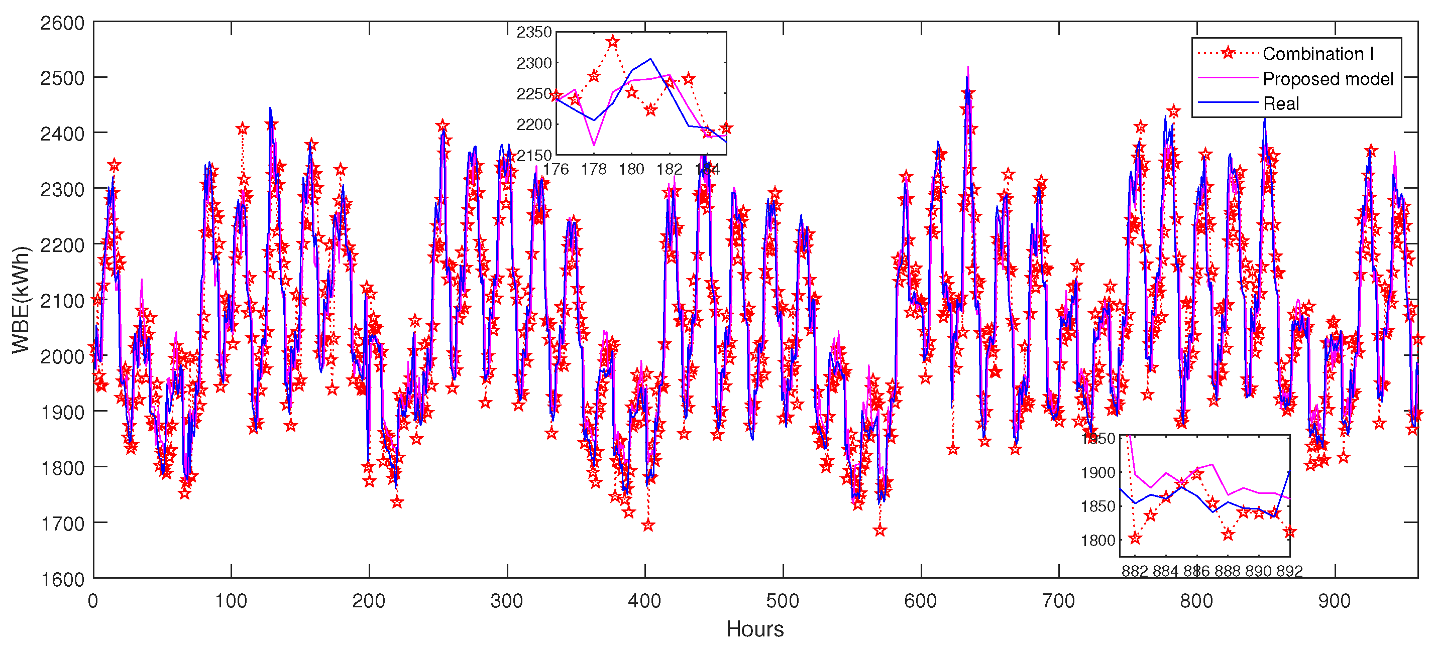
3.3. Campus Building Case B

3.3.1. Description of Target and Source Buildings

Different from case A, a campus building’s daily energy usage data in China is selected for model validation. In benchmark case and case A, a public dataset from ASHRAE that contains more than 1000 buildings is treated as a candidate building pool for similar building selection. In order to prevent excessive differences in building datasets due to different regions, populations, and operation modes, other buildings in the local building group are used for small-scale knowledge transfer in this case study. Compared to hourly data, the daily data have less regularity in peak and valley cycles, and the effectiveness of data clustering is investigated through this case.

The building of Electrical Information Engineering (EIE) at Jiangsu University, China, is selected as the target building. It has five floors, approximately 10,000 square meters in total. The other three buildings in the building group are selected as candidate source buildings (S1–S3). The top view of the building group and the outside of target building are both shown in Figure 14.

The electrical loads come from the database of the Energy Center of Jiangsu University, and the relevant meteorological data are collected from the website (WheatA V1.5.7j platform). The target building selects 600 days of data from 2018 to 2019 for model construction, and the division ratio of training/validating/testing is 1:1:8 by time series. The time series of the target building’s energy loads and corresponding data division are shown in Figure 15. For candidate source buildings, 987 sets of daily data per building from January 2016 to October 2018 are selected. Considering the sensing and recording errors from the field equipment, extra data preprocessing for data outliers and missing values is applied using the interquartile range (IQR) method.

The original input features for data-driven modeling include: mean air temperature, dew point temperature, total cloudiness, holiday flag, sea level pressure, humidity, $y-1$, and $y-2$. After feature selection by Pearson’s method, the dew point temperature is eliminated and the other seven features are selected as model inputs.

3.3.2. Data Clustering for Target Domain and Data Selection from Similar Building

Different from hourly data clustering in the previous case studies, since the regularity of the daily data is not as pronounced as the hourly data, the way of extreme values searching is changed. For the training dataset, according to the energy consumption mode of the campus buildings, the non-working days (weekend) are determined as the energy usage’s valley days, and the day with the most energy consumption is searched as the peak day in a weekly cycle. The one day before and after the peak day are also clustered into peak days together. The data in the validating and testing set are also classified by the KNN method.

For similar building selection, WD metrics are calculated to determine the similarity of the other three candidate buildings in the same group. Results show that the target building has the least distance from the S1 building, whereas the WDs with the other two buildings (S2, S3) are large. Therefore, the S1 building is selected as the source domain building, and, by the LSH method, 277 sets of daily data are picked from S1 as similar data for transfer learning.

3.3.3. Results

After the peak/valley data clustering and transfer learning, the daily electrical load prediction of the target building is performed. To investigate the effect of the proposed method on daily prediction, three different models’ results are recorded in

Table 10. Comparison of prediction before and after data clustering, Elman/iTrAdaboost-Elman.

Model	Clustering	MAE (kWh)	MAPE (%)	RMSE (kWh)
Elman	No	489.16	21.94	646.66
iTrAdaboost-Elman	No	343.12	15.85	433.51
Proposed model	Yes	254.60	12.23	326.04

. The Elman model without data clustering and transfer learning has the worst accuracy (MAE: 489.16 kWh, MAPE: 21.94%, RMSE: 646.66 kWh). The proposed transfer learning model with data clustering still achieves the best accuracy (MAE: 254.60 kWh, MAPE: 12.23%, RMSE: 326.04 kWh). Figure 16 compares the effect of prediction results with and without data clustering.

4. Conclusions

In this study, a clustering-based transfer learning method was proposed to address the problem of insufficient sampling of peak/valley data that affects short-term electrical load prediction performance. Through peak/valley data clustering from target domain and two-stage similar data selection from multi-source domains, the proposed transfer learning iTrAdaboost-Elman model for peak/valley data was built. Three case studies were provided for performance validation. In the benchmark case (public dataset), using only 120 hours’ training data, the proposed model reached a prediction accuracy of 1.96% (MAPE) that was much better than the Elman model (3.80%) and the iTrAdaboost-Elman model without data clustering (2.63%). The effects of data clustering and LSH similar data selection were both investigated. Two other real campus building cases from the USA and China (Case A and B) were then studied to verify the adaptivity and robustness of the model. For different predictive time scales (hourly and daily) and knowledge transfer scopes, the proposed method also had an accuracy advantage compared with other models. Especially for Case B of daily electrical load prediction, in which the energy usage pattern changed and only four buildings were used for similar domain selection, the proposed method still achieved better accuracy than the Elman model (12.23% vs. 21.94%, MAPE) and the iTrAdaboost-Elman model without data clustering (15.85%). For short-term building electrical load forecasting tasks with insufficient data for model training, the proposed method proved superior performance and thus had great application potential in the building energy management system. It should be noted that for proper data clustering, the energy usage cycle must be identifiable. Otherwise, the proposed timestamp and extreme search method would not be effective. Sensitivity analysis of model performance on different time scales and building types will be the next step of our research.

References

1. Dechamps, P. The IEA World Energy Outlook 2022—A brief analysis and implications. Eur. Energy Clim. J. 2023, 11, 100–103. [Google Scholar] [CrossRef]
2. Al-Rakhami, M.; Gumaei, A.; Alsanad, A.; Alamri, A.; Hassan, M.M. An ensemble learning approach for accurate energy load prediction in residential buildings. IEEE Access 2019, 7, 48328–48338. [Google Scholar] [CrossRef]
3. Chen, Z.; Chen, Y.; Xiao, T.; Wang, H.; Hou, P. A novel short-term load forecasting framework based on time-series clustering and early classification algorithm. Energy Build. 2021, 251, 111375. [Google Scholar] [CrossRef]
4. Li, K.; Tian, J.; Xue, W.; Tan, G. Short-term electricity consumption prediction for buildings using data-driven swarm intelligence based ensemble model. Energy Build. 2021, 231, 110558. [Google Scholar] [CrossRef]
5. Filgueiras, D.B.; Coelho da Silva, F.L. A study on the prediction of electricity consumption considering the energy efficiency measures—Applied in case of the Brazilian public sector. Energy Effic. 2023, 16, 94. [Google Scholar] [CrossRef]
6. Zhou, X.; Sun, J.; Tian, Y.; Lu, B.; Hang, Y.; Chen, Q. Hyperspectral technique combined with deep learning algorithm for detection of compound heavy metals in lettuce—ScienceDirect. Food Chem. 2020, 321, 126503. [Google Scholar] [CrossRef]
7. Pavlatos, C.; Makris, E.; Fotis, G.; Vita, V.; Mladenov, V. Enhancing Electrical Load Prediction Using a Bidirectional LSTM Neural Network. Electronics 2023, 12, 4652. [Google Scholar] [CrossRef]
8. Chen, C.; Zhu, W.; Steibel, J.; Siegford, J.; Norton, T.J. Classification of drinking and drinker-playing in pigs by a video-based deep learning method. Biosyst. Eng. 2020, 196, 1. [Google Scholar] [CrossRef]
9. Liu, J.; Abbas, I.; Noor, R.S. Development of Deep Learning-Based Variable Rate Agrochemical Spraying System for Targeted Weeds Control in Strawberry Crop. Agronomy 2021, 11, 1480. [Google Scholar] [CrossRef]
10. Smola, A.J.; Gretton, A.; Borgwardt, K. Maximum mean discrepancy. In Proceedings of the 13th International Conference, ICONIP, Hong Kong, China, 3–6 October 2006; pp. 3–6. [Google Scholar]
11. Panaretos, V.M.; Zemel, Y. Statistical aspects of Wasserstein distances. Annu. Rev. Stat. Appl. 2019, 6, 405–431. [Google Scholar] [CrossRef]
12. Kinney, J.B.; Atwal, G.S. Equitability, mutual information, and the maximal information coefficient. Proc. Natl. Acad. Sci. USA 2014, 111, 3354–3359. [Google Scholar] [CrossRef] [PubMed]
13. Borgwardt, K.M.; Gretton, A.; Rasch, M.J.; Kriegel, H.P.; Schölkopf, B.; Smola, A.J. Integrating structured biological data by kernel maximum mean discrepancy. Bioinformatics 2006, 22, e49–e57. [Google Scholar] [CrossRef] [PubMed]
14. Li, K.; Wei, B.; Tang, Q.; Liu, Y. A data-efficient building electricity load forecasting method based on maximum mean discrepancy and improved TrAdaBoost algorithm. Energies 2022, 15, 8780. [Google Scholar] [CrossRef]
15. Lu, Y.; Wang, G.; Huang, S. A short-term load forecasting model based on mixup and transfer learning. Electr. Power Syst. Res. 2022, 207, 107837. [Google Scholar] [CrossRef]
16. Wei, N.; Yin, C.; Yin, L.; Tan, J.; Liu, J.; Wang, S.; Qiao, W.; Zeng, F. Short-term load forecasting based on WM algorithm and transfer learning model. Appl. Energy 2024, 353, 122087. [Google Scholar] [CrossRef]
17. Yuan, Y.; Chen, Z.; Wang, Z.; Sun, Y.; Chen, Y. Attention mechanism-based transfer learning model for day-ahead energy demand forecasting of shopping mall buildings. Energy 2023, 270, 126878. [Google Scholar] [CrossRef]
18. Tian, Y.; Sehovac, L.; Grolinger, K. Similarity-based chained transfer learning for energy forecasting with big data. IEEE Access 2019, 7, 139895–139908. [Google Scholar] [CrossRef]
19. Li, Y.; Bao, T.; Chen, H.; Zhang, K.; Shu, X.; Chen, Z.; Hu, Y. A large-scale sensor missing data imputation framework for dams using deep learning and transfer learning strategy. Measurement 2021, 178, 109377. [Google Scholar] [CrossRef]
20. Gao, N.; Shao, W.; Rahaman, M.S.; Zhai, J.; David, K.; Salim, F.D. Transfer learning for thermal comfort prediction in multiple cities. Build. Environ. 2021, 195, 107725. [Google Scholar] [CrossRef]
21. Li, A.; Xiao, F.; Fan, C.; Hu, M. Development of an ANN-based building energy model for information-poor buildings using transfer learning. Build. Simul. 2020, 14, 1–13. [Google Scholar] [CrossRef]
22. Pardamean, B.; Muljo, H.H.; Cenggoro, T.W.; Chandra, B.J.; Rahutomo, R. Using transfer learning for smart building management system. J. Big Data 2019, 6, 1–12. [Google Scholar] [CrossRef]
23. Gao, Y.; Ruan, Y.; Fang, C.; Yin, S. Deep learning and transfer learning models of energy consumption forecasting for a building with poor information data. Energy Build. 2020, 223, 110156. [Google Scholar] [CrossRef]
24. Pinto, G.; Wang, Z.; Roy, A.; Hong, T.; Capozzoli, A. Transfer learning for smart buildings: A critical review of algorithms, applications, and future perspectives. Adv. Appl. Energy 2022, 5, 100084. [Google Scholar] [CrossRef]
25. Zeng, P.; Sheng, C.; Jin, M. A learning framework based on weighted knowledge transfer for holiday load forecasting. J. Mod. Power Syst. Clean Energy 2019, 7, 329–339. [Google Scholar] [CrossRef]
26. Li, G.; Wu, Y.; Liu, J.; Fang, X.; Wang, Z. Performance evaluation of short-term cross-building energy predictions using deep transfer learning strategies. Energy Build. 2022, 275, 112461. [Google Scholar] [CrossRef]
27. Li, Z.; Liu, B.; Xiao, Y. Cluster and dynamic-TrAdaBoost-based transfer learning for text classification. In Proceedings of the 13th International Conference on Natural Computation, Fuzzy Systems and Knowledge Discovery (ICNC-FSKD), Guilin, China, 29–31 July 2017; IEEE: New York, NY, USA, 2017; pp. 2291–2295. [Google Scholar]
28. Tong, X.; Xu, X.; Huang, S.L.; Zheng, L. A mathematical framework for quantifying transferability in multi-source transfer learning. Adv. Neural Inf. Process. Syst. 2021, 34, 26103–26116. [Google Scholar]
29. Lu, H.; Wu, J.; Ruan, Y.; Qian, F.; Meng, H.; Gao, Y.; Xu, T. A multi-source transfer learning model based on LSTM and domain adaptation for building energy prediction. Int. J. Electr. Power Energy Syst. 2023, 149, 109024. [Google Scholar] [CrossRef]
30. Wei, B.; Li, K.; Zhou, S.; Xue, W.; Tan, G. An instance based multi-source transfer learning strategy for building’s short-term electricity loads prediction under sparse data scenarios. J. Build. Eng. 2024, 85, 108713. [Google Scholar] [CrossRef]
31. Qian, F.; Ruan, Y.; Lu, H.; Meng, H.; Xu, T. Enhancing source domain availability through data and feature transfer learning for building power load forecasting. In Building Simulation; Springer: Berlin/Heidelberg, Germany, 2024; pp. 1–14. [Google Scholar]
32. Li, K.; Zhang, J.; Chen, X.; Xue, W. Building’s hourly electrical load prediction based on data clustering and ensemble learning strategy. Energy Build. 2022, 261, 111943. [Google Scholar] [CrossRef]
33. Wu, X.; Zhou, J.; Wu, B.; Sun, J.; Dai, C. Identification of tea varieties by mid-infrared diffuse reflectance spectroscopy coupled with a possibilistic fuzzy c-means clustering with a fuzzy covariance matrix. J. Food Process. Eng. 2019, 42, e13298. [Google Scholar] [CrossRef]
34. Li, L. Combining Transfer Learning and Ensemble Algorithms for Improved Citrus Leaf Disease Classification. Agriculture 2024, 14, 1549. [Google Scholar] [CrossRef]
35. Dai, W.; Yang, Q.; Xue, G.R.; Yu, Y. Boosting for transfer learning. In Proceedings of the 24th International Conference on Machine Learning, Corvallis, OR, USA, 20–24 June 2007; pp. 193–200. [Google Scholar]
36. Elman, J.L. Finding structure in time. Cogn. Sci. 1990, 14, 179–211. [Google Scholar] [CrossRef]
37. Shen, T.; Zou, X.; Shi, J.; Li, Z.; Huang, X.; Yiwei, X.; Wu, C. Determination geographical origin and flavonoids content of goji berry using near-infrared spectroscopy and chemometrics. Food Anal. Methods 2016, 9, 68–79. [Google Scholar]
38. Che, J.; Wang, J.; Tang, Y. Optimal training subset in a support vector regression electric load forecasting model. Appl. Soft Comput. 2012, 12, 1523–1531. [Google Scholar] [CrossRef]
39. Andoni, A.; Indyk, P.; Nguyen, H.L.; Razenshteyn, I. Beyond locality-sensitive hashing. In Proceedings of the Twenty-Fifth Annual ACM-SIAM Symposium on Discrete Algorithms, SIAM, Portland, OR, USA, 5–7 January 2014; pp. 1018–1028. [Google Scholar]
40. Kalantari, I.; McDonald, G. A data structure and an algorithm for the nearest point problem. IEEE Trans. Softw. Eng. 1983, 5, 631–634. [Google Scholar] [CrossRef]
41. Ohlsson, M.B.; Peterson, C.O.; Pi, H.; Rognvaldsson, T.S.; Soderberg, B.P. Predicting System Loads with Artificial Neural Networks—Methods and Results from The Great Energy Predictor Shootout. Ashrae-Trans. Am. Soc. Heat. Refrig. Airconditioning Engin. 1994, 100, 1063–1074. [Google Scholar]
42. Huang, D.; He, S.; He, X.; Zhu, X. Prediction of wind loads on high-rise building using a BP neural network combined with POD. J. Wind. Eng. Ind. Aerodyn. 2017, 170, 1–17. [Google Scholar]
43. Liu, C.; Sun, B.; Zhang, C.; Li, F. A hybrid prediction model for residential electricity consumption using holt-winters and extreme learning machine. Appl. Energy 2020, 275, 115383. [Google Scholar] [CrossRef]
44. Wang, Z.; Wang, Y.; Zeng, R.; Srinivasan, R.S.; Ahrentzen, S. Random Forest based hourly building energy prediction. Energy Build. 2018, 171, 11–25. [Google Scholar] [CrossRef]
45. Zhang, A.; Zhang, L. RBF neural networks for the prediction of building interference effects. Comput. Struct. 2004, 82, 2333–2339. [Google Scholar] [CrossRef]
46. Zhou, X.; Lin, W.; Kumar, R.; Cui, P.; Ma, Z. A data-driven strategy using long short term memory models and reinforcement learning to predict building electricity consumption. Appl. Energy 2022, 306, 118078. [Google Scholar] [CrossRef]
Figure 1. Schematic of the iTrAdaboost-Elman model.
Energies 18 00686 g001
Figure 2. Peak and valley clustering and supervised KNN clustering method.
Energies 18 00686 g002
Figure 3. General framework of the study.
Energies 18 00686 g003
Figure 4. Results of Pearson correlation analysis, benchmark case.
Energies 18 00686 g004
Figure 5. Hourly electrical loads’ time series from target building, benchmark case.
Energies 18 00686 g005
Figure 6. The clustered result of 120 hours’ training data from target domain, benchmark case.
Energies 18 00686 g006
Figure 7. Effect of similar data selection by LSH (left: before LSH, right: after LSH), T-SNE, benchmark case.
Energies 18 00686 g007
Figure 8. Prediction results of the proposed model, benchmark case.
Energies 18 00686 g008
Figure 9. Fitted scatter validation plots of predictions (left: Elman, right: proposed model), benchmark case.
Energies 18 00686 g009
Figure 10. Prediction results before and after data clustering, iTrAdaboost-Elman, benchmark case.
Energies 18 00686 g010
Figure 11. Outside of Information Technology Center building, University of Wyoming.
Energies 18 00686 g011
Figure 12. Comparison of prediction results for the proposed model and three combinations, iTrAdaboost-Elman, case A.
Energies 18 00686 g012
Figure 13. Prediction results with and without the proposed data clustering method, iTrAdaboost-Elman, case A.
Energies 18 00686 g013
Figure 14. The outside of target building and the top view of the building group, Jiangsu University.
Energies 18 00686 g014
Figure 15. Daily electrical loads’ time series from target building, case B.
Energies 18 00686 g015
Figure 16. Prediction results with and without data clustering, iTrAdaboost-Elman, case B.
Energies 18 00686 g016