AI-Based Clustering of Numerical Flow Fields for Accelerating the Optimization of an Axial Turbine

Abstract

The growing number of Renewable Energy Sources has increased the demand for innovative and high-performing turbine designs. Due to the increase in computing resources over recent years, numerical optimization using Evolutionary Algorithms (EAs) has become established. Nevertheless, EAs require many expensive Computational Fluid Dynamics (CFD) simulations, and more computational resources are needed with an increasing number of design parameters. In this work, an adapted optimization algorithm is introduced. By employing an Artificial Intelligence (AI)-based design assistant, turbines with a similar flow field are clustered into groups and provide a dataset to train AI models. These AI models can predict the flow field’s clustering before a CFD simulation is performed. The turbine’s efficiency and cavitation volume are predicted by analyzing the turbine’s properties inside the predicted clustering group. Turbines with properties below a certain threshold are not CFD-simulated but estimated by the design assistant. By this procedure, currently, more than 30% of the CFD simulations are avoided, significantly reducing computational costs and accelerating the overall optimization workflow.

1. Introduction

The demand for Renewable Energy Sources (RESs) has drastically grown in recent years to reduce the use of conventional energy resources (such as fossil fuels) for power generation. In 2023, renewable energies sourced almost one-seventh of the world’s primary energy. Additionally, until the end of 2050, up to 80% of the energy is expected to be produced by RESs in the European Union. Hydropower accounted for almost 47% of all renewable energies produced in 2023 [1]. The contributions of other RESs, such as wind and solar, have also grown. However, such undispatchable RESs threaten grid stability. Hydropower can play a key role in providing emission-free RESs and regulating and balancing the grid in both the short and long term [2]. These grid requirements demand durable, flexible, and innovative turbine designs.

The increase in computing resources over the last few years provides the opportunity to design hydraulic machinery in an automated manner [3,4]. Besides the fluid mechanical properties, a hydraulic machine has to deal with unsteady mechanical loads leading to vibrations. In that sense, it is beneficial to optimize the machines simultaneously for fluid and structure mechanics [5]. These optimization tasks are computationally expensive and challenging due to the high number of time-consuming simulations required. The computational burden of the optimization task is generally non-linear with each added design degree of freedom (DOF) [6,7]. Each added DOF contributes to characterizing the “dimensionality” of the optimization task, which hence becomes more and more resource-intensive. It is also known that EAs need many evaluations of the problem to be optimized. In addition, many of the evaluations are only used during the ongoing optimization. It is not always necessary to have an exact fitness value because the optimizer decides depending on better or worse tendencies, disregarding the differences [8,9].

Recent developments in computational methods, and advancements in hardware technology, have led to a drastic reduction in computational costs. Consequently, optimizations based on EAs generate much larger databases with an increased number of DOFs. This abundant data availability has enabled the integration of AI into the engineering discipline. Recently, this integration has rapidly accelerated in the field of fluid dynamics and design optimization, with numerous articles demonstrating the potential of Machine Learning (ML) in fluid dynamics [10,11,12].

An optimization task is complex and often involves a significant amount of high-dimensional data. ML offers effective approaches to address the “curse of dimensionality”. Several ML techniques have demonstrated excellent performance in dimensionality reduction. Popular deep learning techniques include Deep Convolutional Networks (DCNs) [13,14], Autoencoders (AEs) [15], Generative Adversarial Networks (GANs) [16,17,18], and Long Short-Term Memorys (LSTMs) [19,20]. Among these, AE technology has shown exceptional results in past case studies. Some past success stories are presented in [21,22]. This method extracts the essential building block information and projects it into an optimal low-dimensional space, known as the latent space. It preserves crucial information, enabling the reconstruction of the original data.

Following dimensionality reduction techniques, the clusters based on similar traits and behaviors are identified using clustering methods, also termed community detection. The community detection methods are classified into two major classes: (1) deep learning methods and (2) traditional methods. The latter methods capture the relationships in a shallow, easier-to-understand manner. These methods mostly employ strategies based on statistical and/or mathematical functions. Some such methods are random-walk-based dynamical clustering [23], density-based algorithms, and probabilistic model-based statistical inference methods [24]. In the former case, deep learning approaches are utilized for higher-order dimensionality reductions for the data, followed by some Euclidean-based clustering methods such as k-means clustering. Spectral Clustering has gained significant traction in recent years due to its versatility and effectiveness across various fields, including engineering, statistics, and natural sciences. Unlike traditional clustering algorithms, Spectral Clustering leverages the eigenvalues and eigenvectors of a similarity matrix derived from the data, allowing it to capture complex structures and relationships within data. The algorithm’s ability to handle non-convex clusters and its robustness against noise make it easier to implement and operate than other clustering techniques. Its applications extend to text clustering, recommendation systems, and traffic analysis, showcasing its broad utility and addressing diverse challenges in ML [25,26,27].

Building upon these advancements, this work targets the prediction of fitness values within the optimization of an axial turbine with a two-step fitness evaluation based on ML. In the first step, an AE is used to obtain the reduced-dimensionality flow field. In the second step, the flow fields are clustered using Spectral Clustering, again based on the dimensionality-reduced flow fields. This approach has been integrated into the in-house design system Design Tool Object-Oriented (dtOO) [3].

The main contributions of the presented work are as follows:

• Advanced pre-processing of the flow field and pressure data across the turbine blade.
• Encoding the processed data into the latent vector representation.
• Clustering the latent represented data into different clusters using Spectral Clustering.
• Evaluation of the fitness values of the turbines based on advanced clustering of the data.
• Integrating the approach into the in-house design system.

This paper is structured as follows: Section 2 deals with the background information, including details of dtOO, Non-Dominated Sorting Genetic Algorithm II (NSGA-II), and Spectral Clustering. Section 3 gives details about the problem definition and how AI is implemented to modify the workflow in dtOO. Section 4 presents the current study’s results. Section 5 and Section 6 provide discussions and concluding remarks.

2. Background

In this section, a comprehensive overview of the key components and methodologies underpinning this research is provided. The in-house dtOO framework [3] is described in detail, including its dependencies and code structure, which form the foundation of the optimization process. Additionally, the geometrical definition of the axial turbine is explained, which gives a clear picture of the design space being explored. A brief introduction of the optimization algorithm employed is provided, highlighting its role in navigating the complex design landscape. Finally, the clustering mechanism is discussed as a vital element in analyzing and categorizing design variants.

2.1. Design Framework dtOO

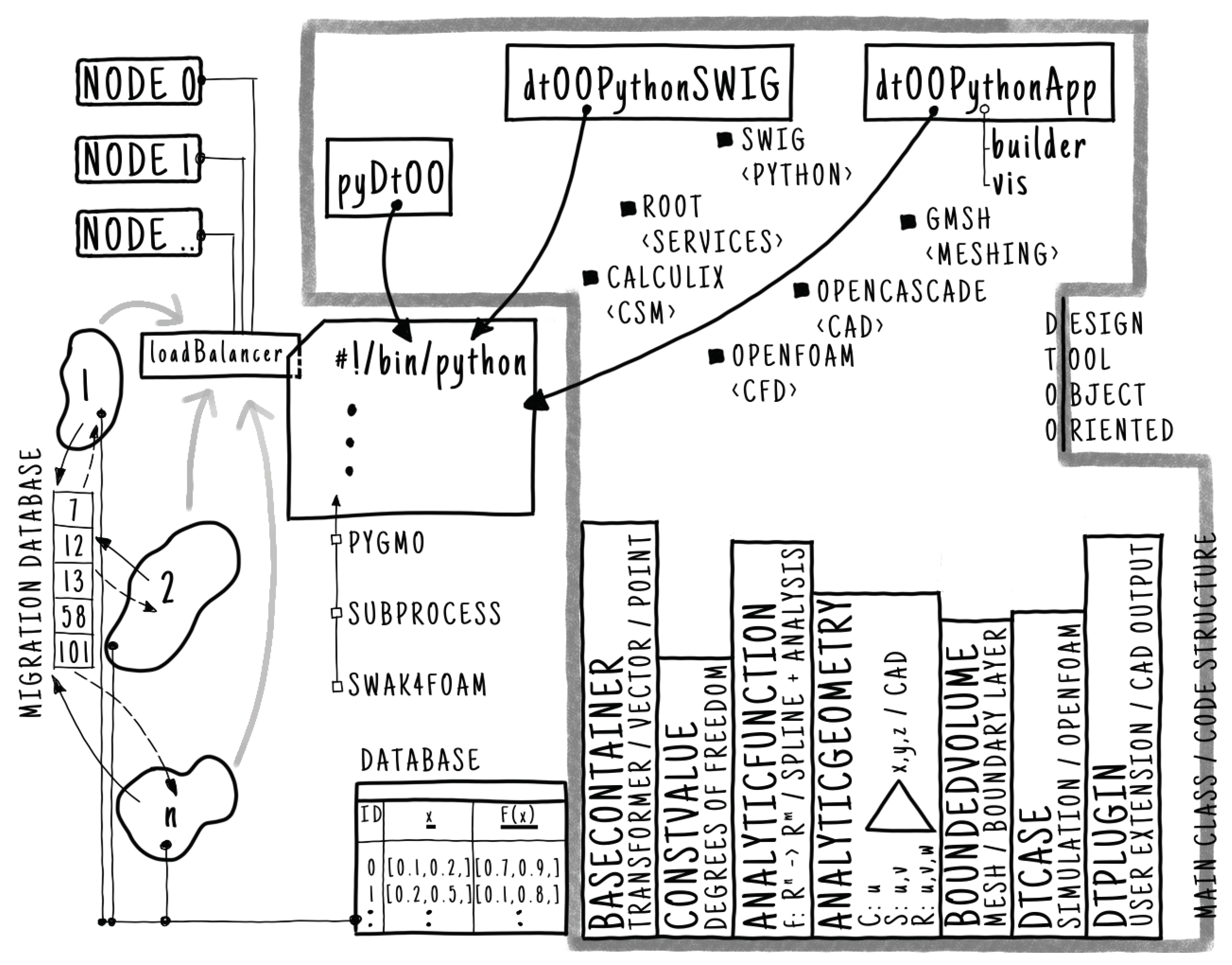
The package dtOO was developed to have a framework that is free of license costs, flexible and extendable, and can deal with hydraulic machines. Figure 1 presents an overview of dtOO, including its main dependencies, provided packages, and additional implementation details. The main part written in C++ is included in the figure’s thick gray-framed part. The main dependencies in dtOO are listed with a leading filled square symbol, including their main functions within <>-symbols. The left part of Figure 1, outside of the gray frame, schematically visualizes the workflow of a typical optimization procedure. The main Python process (black rectangle with Shebang line and vertical dots) uses the island model (visualized as a group of three freely shaped islands) and two databases to distribute candidates to computing nodes (rounded rectangles in the top left corner).

The black-framed package dtOOPythonSWIG interfaces with Python to import and use the framework in a Python script. The other two packages, dtOOPythonApp and pyDtOO, provide application builder algorithms and support evaluations of Open Field Operation And Manipulation (OpenFOAM) [28], respectively. The user can access predefined Python classes for default components, e.g., runners, draft tubes, guide vanes, mesh topologies, and steady-state simulation cases, by importing the builder subpackage. The second vis subpackage provides an interface to ParaVIEW to visually investigate the created geometries. The packages can be imported to the Python script, indicated by the solid black arrows starting at the packages.

The dtOO’s source code is object-oriented, consisting of main classes shown in the bottom right part of Figure 1. The black-framed vertically lettered boxes include the class name in the first line of the box, followed by its main function and/or additional comments. Instances of each class except baseContainer are collected in Standard Template Library (STL)-like containers. A container’s element can be accessed either by its label or its index. The baseContainer is different because it collects different classes, e.g., two- and three-dimensional vectors as well as points and transformers. To change a parameterized geometry, the user or the optimizer changes the DOFs’ values (instances of constValue). The geometry is then a collection of curves, surfaces, and regions or, respectively, a mapping from one dimension $\left(u\right)$, two dimensions $(u,v)$, or three dimensions $(u,v,w)$ into the physical three-dimensional coordinate system $(x,y,z)$. The mapping for a curve, surface, and region is indicated in Figure 1 by C, S, and R, respectively. All these geometries are collected as instances of analyticGeometry and, therefore, provide Computer-Aided Design (CAD) functionalities. All other mathematic functions necessary for defining, e.g., a distribution of nodes for meshing or a thickness distribution are represented as an instance of analyticFunction. Generally, the analyticFunction is an arbitrary function f mapping from ${\mathbb{R}}^n$ to ${\mathbb{R}}^m$. This expression is also noted in the corresponding vertical box in Figure 1. In the end, a geometry that can be meshed is a collection of instances of analyticFunction and analyticGeometry within an object of boundedVolume. This class provides meshing tools, e.g., the creation of a boundary layer and an interface to gmsh that finally creates the mesh. This mesh is transferred to an instance of dtCase, which supports the setup of a simulation case. Typically, this is performed using OpenFOAM. Besides the object-oriented structure, instances of dtPlugin can also extend the framework. It is easy to write a shared-object library with its desired user-intended extension code and load it within the framework. This prevents recompilation of the framework.

The dependency swig is mandatory for the Python interface. The geometry representation (OpenCASCADE) within the framework is directly interfaced with the meshing representation and algorithms (gmsh). During the meshing procedure, points need to be reparameterized on curves or surfaces. These are typically iterative procedures implemented by minimization tasks supported by the dependency root. If additional Computational Solid Mechanics (CSM) simulations are performed, CalculiX [29] provides the von Mises stress field.

Additional dependencies that occur due to the executed Python script are given in the figure with an empty leading square symbol and are also connected to the black-framed box with a Shebang line. These Python dependencies can change and are dependent on the script file.

Within Figure 1, the island model [30,31] and the distribution to the nodes are schematically shown on the left side, outside of the gray-framed structure. The freely shaped islands optimize the problem using an EA. During the optimization of one generation, there is no communication with the other islands; the migration occurs only after a predefined number of generations. The black solid and dashed lines between the islands and the migration database indicate this sending procedure of candidates. To have an asynchronous migration, migrants are stored in a migration database. The islands can send and receive candidates from the database whenever necessary. Within the figure, the migration database contains some unique individual IDs exchanged during an ongoing optimization.

The second database is connected to each island, and stores all evaluated candidates. The figure shows this connection by the straight, black, solid lines in the bottom left corner. This database enables post-processing as well as migration techniques that also pick from this database and not only from the current existing generation. The database in Figure 1 is filled with data of two candidates, including their ID, DOFs, and fitness values.

The thick gray arrows represent the delegation of the simulations to a loadBalancer object. One of these arrows means one channel constantly sends candidates while the optimization is ongoing. Due to the simulations’ unequal duration and multiple simulations per candidate evaluation, the loadBalancer distributes the jobs to the nodes. The input from the islands is processed using a first-in-first-out principle. This means that an island waits until the desired candidate’s evaluation is finished.

2.2. Geometrical Setup of Axial Turbine

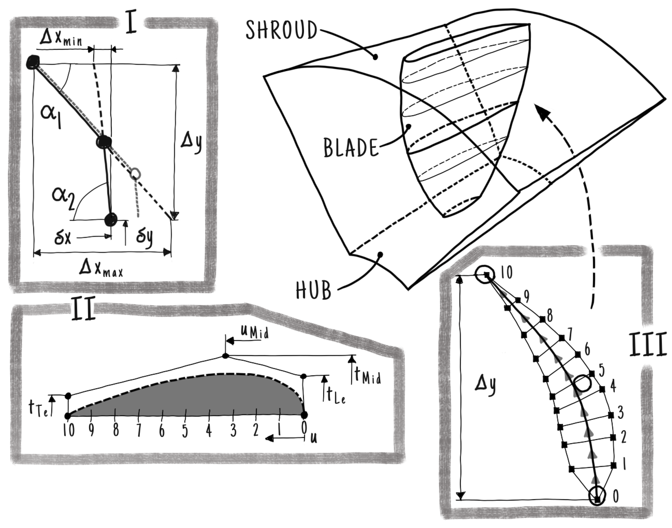
Figure 2 shows the runner of the test case and its creation procedure. The three-dimensional shape of the hydraulic machine is parameterized in dtOO using the Python interface dtOOPythonSWIG and the dtOOPythonApp builder algorithm library. Sketch I defines the mean line, including its DOFs. It is defined in a two-dimensional frame of reference so that x and y correspond to $\varphi r$ and m, respectively. The coordinates $\varphi r$ and m are the circumferential and meridional directions. In this regard, the DOFs $\Delta x_{max}$, $\Delta x_{min}$, and $\delta x$ correspond to the maximum possible expansion, the minimum possible expansion, and the shift in circumferential direction, respectively. The maximum and minimum expansion in this direction depend on the inlet angle ${\alpha }_1$ and outlet angle ${\alpha }_2$. The extreme values of the extension are the straight lines under one angle. These are indicated in sketch I by the black dashed lines. It is clear that the straight line with inlet angle ${\alpha }_1$ that defines $\Delta x_{max}$ has a vanishing part with outlet angle ${\alpha }_2$; the same applies to $\Delta x_{min}$. The actual blade’s extension is calculated as a weighted average of the two extreme values. Within sketch I, two possible mean lines are the black solid and gray dashed lines. The gray mean line has a higher expansion in the circumferential direction. The DOFs $\Delta y$ and $\delta y$ correspond to the expansion and the shift in the main flow direction of the runner.

In sketch II, the thickness distribution is visualized. The function is defined as a B-Spline curve of second order with five control points. Only a reduced number of the control points’ coordinates are free to move, so that a smooth transition at the leading edge is guaranteed. According to sketch II, the DOFs $t_{Te}$, $u_{Mid}$, $t_{Mid}$, and $t_{Le}$ parameterize the distribution. The u-direction is defined along the curved mean line and the t-direction is perpendicular to it.

Combining the mean line and thickness distribution results in the blade cut, shown in sketch III. The blade cut is generated by dividing the mean line and the thickness distribution into a predefined number of sections. Within sketch III, ten sections are shown. At each section of the mean line, the blade’s thickness is extracted from the thickness distribution and added at this position in a perpendicular direction. In sketch III, the direction from sections zero to ten is indicated with gray arrows; the discrete points after adding the corresponding thickness are shown as black rectangles. These discrete points form the blade cut as a B-Spline. It is still represented in its two-dimensional frame of reference. All two-dimensional blade cuts are combined in a B-Spline surface by adding a constant spanwise coordinate s. The resulting surface is then defined in $\varphi r$-m-s coordinates.

The last step is to map each blade point to its corresponding position in the three-dimensional channel. The blade’s final geometry is not directly constructed. It is created on demand for each point that is necessary during any procedure in the framework. This clearly costs performance, but it prevents the algorithm from failing due to inaccuracies.

2.3. Optimization Algorithm

Described as “A fast and elitist multi-objective genetic algorithm” [32], NSGA-II is designed to solve multi-objective optimization problems efficiently. The algorithm employs an iterative process to evolve a population of solutions, thereby demonstrating its elitism through maintaining high-quality solutions while promoting diversity among them. This application integrates NSGA-II into dtOO using the open-source PyGMO [33] library. The process begins with a population derived from Latin Hypercube Sampling (LHS), refined through k-means clustering to balance diversity and homogeneity. The algorithm sorts the populations’ candidates based on their fitness or, more precisely, on the dominance of two individuals. In case of equal objectives for candidate C and D, C dominates D if at least one objective is better.D. In that sense, the solutions are ranked into Pareto fronts based on this rule. A crowding distance metric ensures diversity within each front by favoring isolated solutions. Genetic operators, including selection, crossover, and mutation, are applied to generate new populations, balancing exploration and exploitation.

2.4. Feature Extraction with AE

An AE is a type of unsupervised learning in the ML paradigm. The network’s input and output are similar, with a low-dimensional bottleneck, also called the latent space. Generally, it consists of two parts: an encoder and a decoder. The encoder represents the high-dimensional input F as lower-dimensional latent data z. The decoder attempts to reconstruct a similar input $F^{\prime }$ from this lower-dimensional latent data z. Thus, an AE learns a compact representation of high-dimensional data. Training an AE involves minimizing the error between the original input F and reconstructed input $F^{\prime }$. Consequently, the hidden layers try to learn good input-compressed representations. In this learning approach, the AE learns to capture the most salient features of the input data F, making them helpful in generating lower-dimensional embeddings for subsequent machine learning algorithms [22].

2.5. Spectral Clustering

Clustering refers to grouping of the individuals based on mutual similarities. Spectral methods refer to a set of algorithms that utilize the eigenvalues and eigenvectors of specifically designed matrices constructed from data. Due to its simplicity and effectiveness, Spectral Clustering is beneficial for many different applications. It is often used with other sophisticated algorithms to enhance performance [34]. Spectral Clustering methods strongly rely on graph networks. Consider $Z=\{z_1,\cdots ,z_n\}$ to be a set of patterns. A complete weighted undirected graph $G(V,W)$ has the set of nodes $V=\{z_1,\cdots ,z_n\}$ corresponding to n patterns and edges defined through the $n\times n$ adjacency (affinity) matrix W, with $w_{ij}$ representing the weight of the edge between node i and node j. If the edges are undirected, the matrix is symmetric and fulfills $w_{ij}=w_{ji}$. The mathematical adjacency relation $w_{ij}$ between two patterns is given as follows:

$$w_{ij}=\left\{\begin{array}{cc}h(z_i,z_j)\hfill & \mathrm{if}i\ne j,\hfill \\ 0\hfill & \mathrm{otherwise}.\hfill \end{array}\right.$$

(1)

The function

$$h(z_i,z_j)=exp\left({\displaystyle \frac{-b(z_i,z_j)}{2{\sigma }^2}}\right)$$

(2)

gives the similarity between patterns [35]. The function b is the dissimilarity between patterns, and $\sigma$ controls the decay rate of h. The degree matrix D is defined as a diagonal matrix whose elements are the degrees of the nodes of G:

$$d_{ij}=\sum _{j=1}^n{w}_{ij}$$

(3)

Within this, the clustering problem can be seen as the graph cut problem [36], where the aim is to separate a set of nodes $S\subset V$ from the complementary set $\tilde{S}=V\backslash S$. This separation is crucial because it allows us to identify distinct groups within the data by minimizing the connections (or weights) between the nodes in set S and those in its complement $\tilde{S}$. The objective of the graph cut problem is to find a division that results in the least total weight of edges connecting the two sets. Thus, this problem is formulated as an optimization problem, aiming to minimize the cut cost defined by the sum of weights of the edges that cross between two sets. This optimization framework provides a powerful method for identifying clusters within the data represented by the graph. This transition effectively connects the concept of complementary sets to the formulation of graph cut problems in clustering. Mathematically, the graph cut problem can be formulated as follows:

$$\mathrm{cut}(S,\tilde{S})=\sum _{z_i\in S,z_j\in \tilde{S}}{w}_{ij}$$

(4)

These cut optimization functions are very complex. They can be relaxed by using spectral concepts of graph analysis. These are given by the Laplacian matrix L and the normalized Laplacian matrix $L_N$, given as follows:

$$L=D-W$$

(5)

$$L_N=D^{-1/2}L{D}^{-1/2}$$

(6)

The latter is a linear operator on G. Shi and Malik [37] provide more details of the clustering method algorithm. Interested authors should refer to [38] for more details about Spectral Clustering.

2.6. Gaussian Process Regression

Random variables described as a joint Gaussian distribution specify a Gaussian Process (GP) and can be used in regression. This work uses Gaussian Process Regression (GPR) to predict the axial turbines’ fitness values. In GPR, prior knowledge is supplemented by the likelihood knowledge of the training data $X=(x_1,x_2,\dots )$ with training output $\mathbf{f}$$=(f_1,f_2,\dots )$ to deliver predictions for unknown data points $X_{*}=(x_{predic{t}_1},x_{predic{t}_2},\dots )$.

A GP is solely described by its mean $m\left(x\right)$ (here set to zero) and the covariance function $k(x,x^{\prime })$, with $x,x^{\prime }\in X$ by

$$\mathit{f}\left(\mathit{x}\right)\sim GP(m\left(x\right),k(x,x^{\prime }))$$

(7)

The covariance function $k(x,x^{\prime })$ describes the covariance between the outputs f, only dependent on the input data x. It characterizes the deviations in output space f depending upon the input data x. Therefore, it determines the characteristics of the possible regression functions for the process. Through element-wise computation of $k(x_{predict},x_{predict}^{\prime })$ for each pair of data points $x_{predict},x_{predict}^{\prime }\in X_{*}$, the covariance matrix $K(X_{*},X_{*})$ is computed. The prior distribution of the probability variables ${\mathbf{f}}_{*}$ of the prediction data $(X_{*},{\mathbf{f}}_{*})$ is normally distributed and given by

$${\mathbf{f}}_{*}\sim \mathcal{N}(\mathbf{0},K(X_{*},X_{*}))$$

(8)

Combining the training data $(X,\mathbf{f})$ with the prediction data $(X_{*},{\mathbf{f}}_{*})$ gives

$$\left[\begin{array}{c}\mathbf{f}\\ {\mathbf{f}}_{*}\end{array}\right]\sim \mathcal{N}\left(\mathbf{0},\left[\begin{array}{cc}K(X,X)& K(X,X_{*})\\ K(X_{*},X)& K(X_{*},X_{*})\end{array}\right]\right)$$

(9)

Conditioning this distribution on the (previously known) training data $(X,\mathbf{f})$ delivers the posterior distribution for the prediction data $(X_{*},{\mathbf{f}}_{*})$:

$${\mathbf{f}}_{*}|X_{*},X,\mathbf{f}\sim \mathcal{N}(K(X_{*},X)K{(X,X)}^{-1}\mathbf{f},K(X_{*},X_{*})-K(X_{*},X)K{(X,X)}^{-1}K(X,X_{*}))$$

(10)

For more detailed information, refer to [39].

3. Problem’s Description and Workflow’s Modification

This section provides a detailed overview of the problem of optimizing axial turbines, focusing on how the fitness value is defined and evaluated. Additionally, this section highlights the significant changes made in the optimization workflow.

3.1. Axial Turbine

An axial turbine with four blades is chosen as a test case. The quarter section of the axial turbine is shown in Figure 2. The geometry consists of a runner channel with a blade and a hub and shroud with radius 0.5 m and 1.9 m, respectively. This test case is evaluated using three different load conditions: nominal, part, and full load. The volume flow rates at part and full load are set to $0.85$ and $1.15$ times the discharge at nominal load, respectively.

3.2. Numerical Setup and Optimization Problem

The framework dtOO provides support for hybrid meshes. This means the axial turbine is meshed with tetrahedrons, prisms, pyramids, and hexahedrons. The candidates are meshed with a structured mesh block and prism layers to make correct predictions of the pressure and shear forces on the blade, hub, and shroud. The structured mesh block is necessary for correctly predicting the flow surrounding the blade and remaining flexible due to filling up the remaining blade-free channel with tetrahedrons. The prism layers maintain the benefits of unstructured meshes, as the hub and shroud sections vary strongly during the optimization process. CFD simulations for the evaluations are performed with OpenFOAM using version $v2206$. The turbine’s rotational speed is set to 72 min⁻¹, and the pressure at the outlet is set at 0 Pa. The k-w-SST turbulence model is used in the performed CFD simulations. Inlet velocities and turbulence quantities are interpolated from an intake section to the actual inlet of the turbine to achieve real-life inflow conditions.

The fitness function for the axial turbine is a multi-dimensional function $\underline{f}$, consisting of three values extracted from the CFD simulation. Each turbine is evaluated based on an averaged efficiency

$$\overline{\eta }={\displaystyle \frac{1}{3}}({\eta }_{pl}+{\eta }_n+{\eta }_{fl})$$

(11)

and cavitation volume

$$\overline{V_{cav}}={\displaystyle \frac{1}{3}}(F_V\left(V_{cav,pl}\right)+F_V\left(V_{cav,n}\right)+F_V\left(V_{cav,fl}\right))$$

(12)

as well as the deviation in head

$$\Delta H=F_H(\Delta H_n)$$

(13)

for the nominal operating condition. The functions $F_V$ and $F_H$ are penalty functions. The fitness function

$$\underline{f}=\left[1-\overline{\eta },\overline{V_{cav}},\Delta H\right]$$

(14)

is an “averaged fitness” in all operating points except for the head.

A Morris sensitivity study of the given test case of the axial turbine was performed using the classical method and a deep learning-assisted method in the literature [40].

3.3. Modification of the Optimization Procedure

This work introduces an AI-based design assistant to optimize the problem. Simply put, the design assistant extracts the features of the problem’s flow fields, creates clusters, and approximates their fitness values. Each flow field is divided into Flow Areas (FAs) surrounding the blade. The results of each FA are then clustered. These clustering results form the Cluster ID (CI) that describes the flow field of a candidate. Undesired flows are identifiable depending on their CI. A Neural Network (NN) is implemented for each FA to detect turbines with unwanted flow properties before simulation. Unwanted flow fields refer to flows with a high cavitation volume and/or low efficiency. The NNs predict the CI based on the candidate’s DOFs. These NNs prevent turbines with unwanted flow fields beforehand, avoiding time-consuming simulations. Each new candidate suggested by the optimization algorithm is then evaluated based on its cluster position to determine whether a simulation is necessary.

3.3.1. Flow Field Extraction

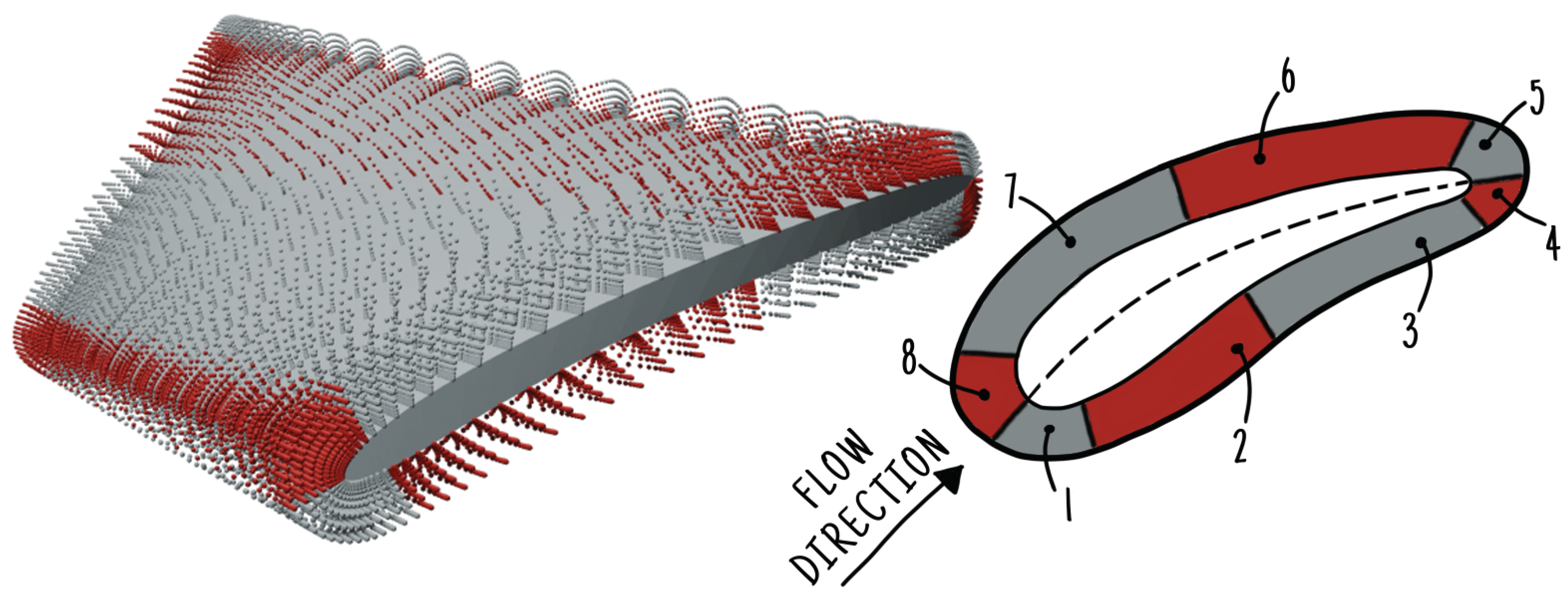
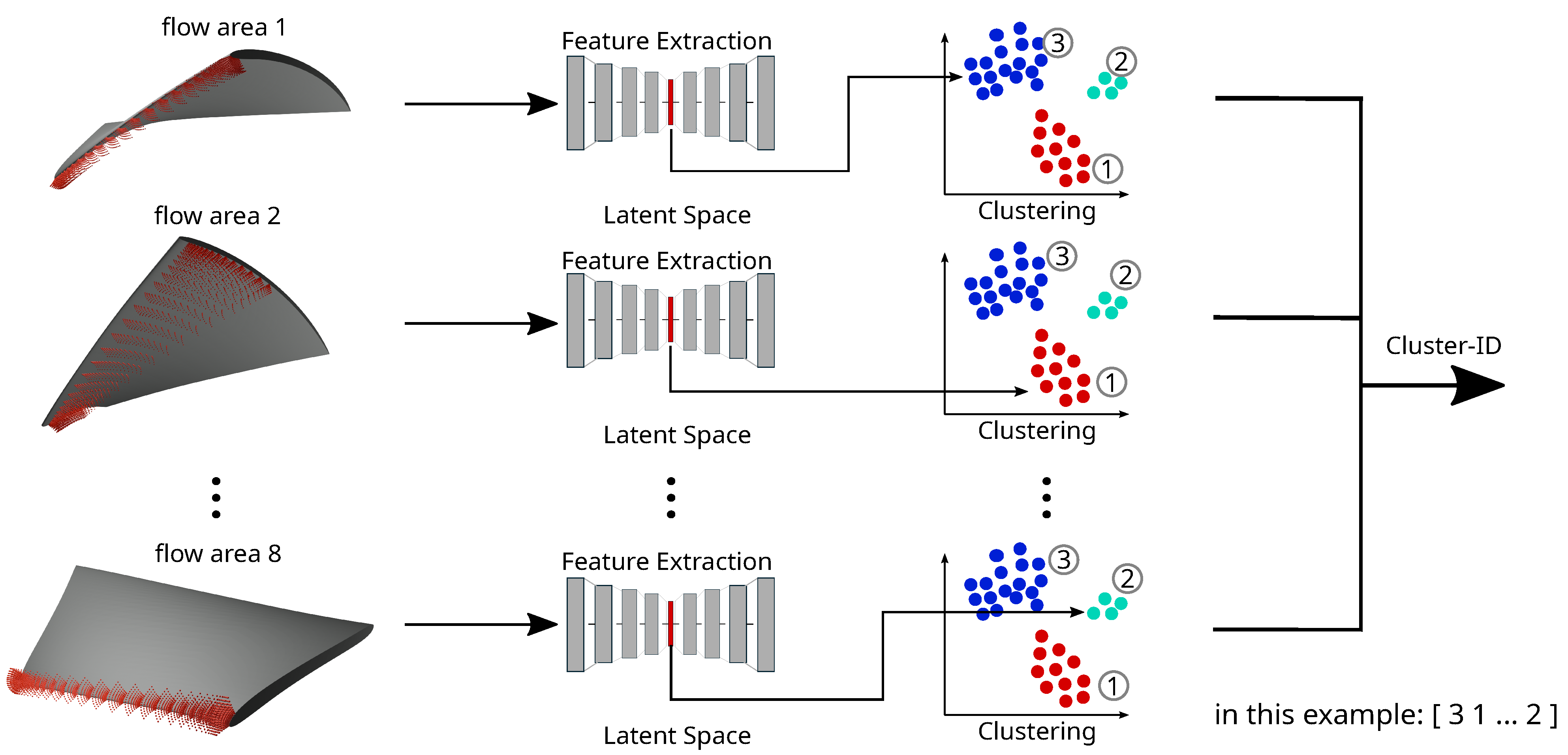
The flow field of a turbine is extracted at predefined coordinates relative to the turbine’s blade. Since the blade geometry of each turbine varies through the optimization process, the coordinates must depend on the blade geometry. They cannot remain fixed in space to ensure comparability between different turbine geometries. Therefore, the velocity and pressure data are extracted for each cell within the hexahedral boundary layer of the hybrid mesh. These cells maintain logically the same position in relation to the blade. As shown in Figure 3, the flow field around the blade is divided into eight FAs. This division enables the comparison of flow phenomena corresponding to specific blade regions, such as the leading edge, across different simulations. As a result, eight distinct tensors with flow field information are obtained per simulation.

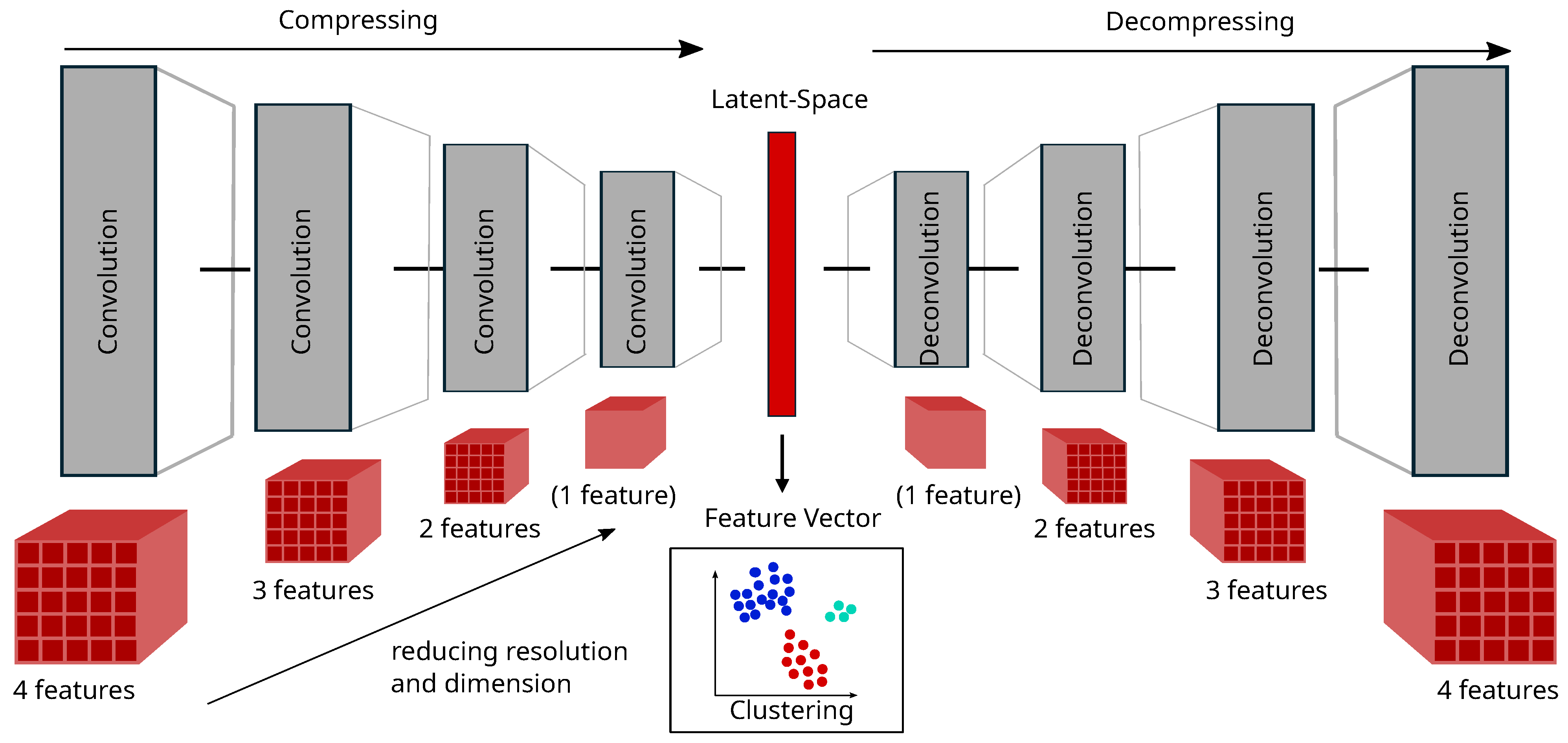
Pressure and velocity data are extracted for each coordinate in the hexahedral mesh area of the test case. Therefore, a four-dimensional tensor consisting of the extracted data and the three spatial coordinates is received. Since three different operating points are considered, one candidate evaluation contains three CFD simulations to receive its fitness values in the optimization process. The three simulation results are combined by stacking up the tensors for each operating point in their last dimension to compare the flow fields. Due to this, turbines within the same cluster share similar flow fields in all three operating points. Before clustering, a three-dimensional convolutional AE converts each tensor into a low-dimensional space. Both the encoder and decoder use four layers, as shown in Figure 4. The feature vector is received within the latent space of the AE. As each flow field is divided into eight FAs, eight distinct feature vectors per turbine are obtained.

Each AE is trained using approximately $65\%$ of turbines as training data and the rest as validation data, randomly chosen. Before starting the optimization, each AE is pretrained by the initialization dataset for 40 iterations. As an optimizer, the Adam algorithm implemented in PyTorch is used. As a loss function, the mean square error using the $L_2$-norm is employed. The learning rate is set to $0.001$ and the batch size equals two. As an activation function, the sigmoid function is employed. The loss gradient is computed in each iteration using backpropagation on the training data. Eight turbines are randomly selected from the validation dataset to determine the validation error. Every time the current validation error is smaller than the previous smallest validation error, the model weights are saved. During optimization, the AEs are retrained for ten iterations after every ten generations in the NSGA-II.

Table 1. AE training parameters.

Training Data	Validation Data	Learning Rate	Batch Size	Optimizer
$65\%$	$35\%$	0.001	2	Adam

summarizes the parameters to set up the AE.

3.3.2. Clustering

One clustering task per FA compares different turbines regarding their flow in this FA. These tasks are conducted independently for each FA. Consequently, eight different clustering tasks must be completed in total, Figure 5. Each turbine is assigned to one cluster per FA, resulting in eight cluster assignments per turbine. For each FA, a turbine receives a Cluster Number (CN) within the range [0, k], with the Amount of Clusters (k) being the maximum number of clusters in this FA. These eight CNs collectively form the CI, which uniquely identifies the turbine’s flow group assignments across all FAs. The flow fields of two turbines are considered similar if their CNs are identical across all eight FAs, resulting in matching CIs. However, it is essential to note that turbines with the same CI do not necessarily have identical flow fields. Instead, their flow fields share common properties, as determined by the clustering algorithm.

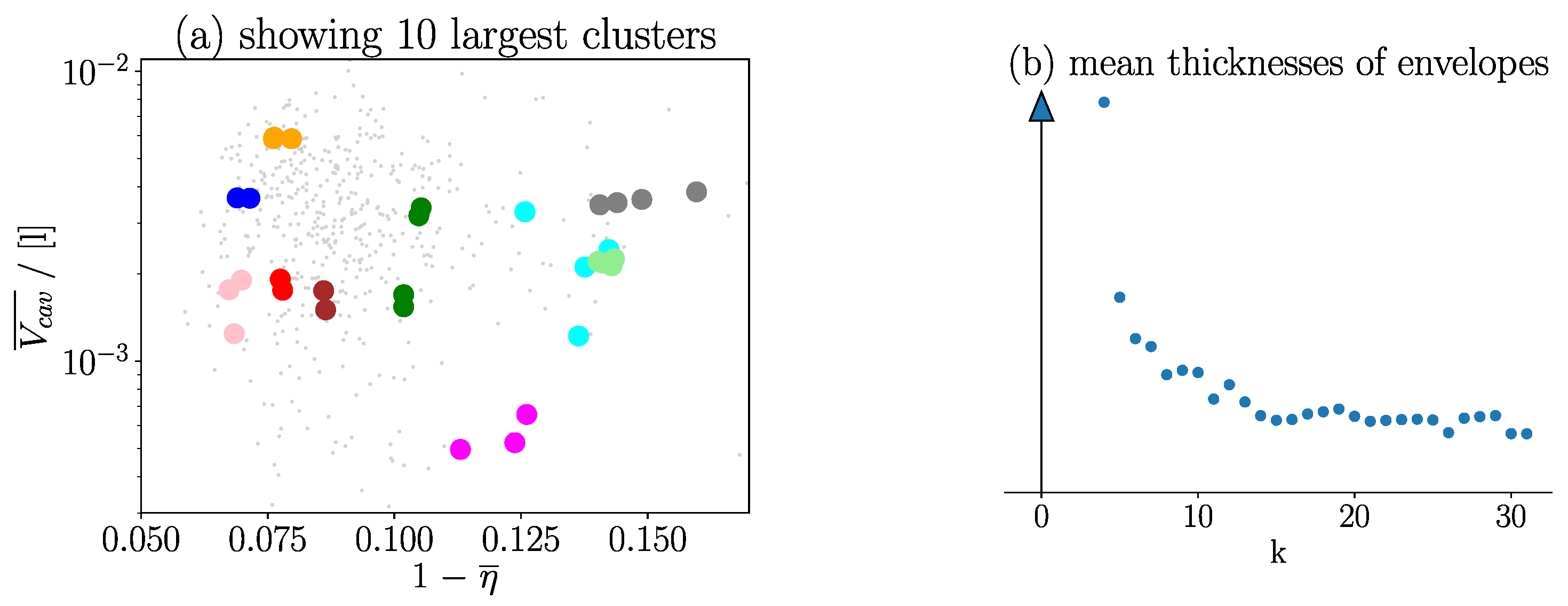
3.4. Investigation of Turbines That Share the Same CI

As mentioned earlier, turbines with equal CIs also share a similar flow field. Investigating the properties of these turbines shows that they also share similar fitness values. An exact assignment of CI to fitness properties is impossible, but Figure 6 indicates that the CI can deliver an approximation. The presented result on the left side of Figure 6 is based on a dataset of 500 turbines. The clustering algorithm’s behavior is affected by the freely determinable parameter k. A higher value of k enables the algorithm to distinguish more precisely between different flows. Generally, flow fields with the same CI share more similar fitness values. However, a higher k also leads to more CIs in the dataset, meaning that fewer simulations share the same CI.

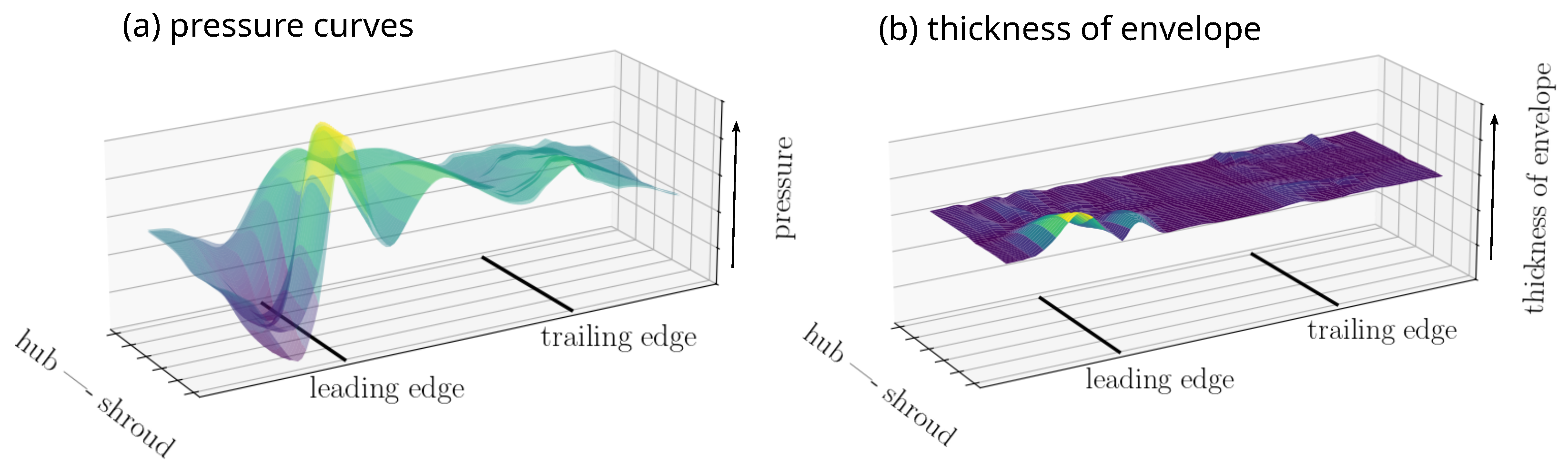
The similarity of flow fields sharing the same CI is compared for different values of k to investigate the influence of k on the clustering quality. The pressure values on the blade generated by the flow are extracted to define a criterion. All pressure surfaces of candidates with equal CIs are superposed. See the left side of Figure 7. Subsequently, for each CI, the envelope of these pressure surfaces is determined by computing the upper and lower limits of these surfaces. The mean thickness of this envelope determines the quality of the clustering. A slimmer envelope indicates more similar flow fields sharing the same CI. An example of an envelope’s thickness distribution is shown on the right side of Figure 7. Similarly, the average of the thicknesses of all the CIs’ envelopes indicates the quality of a specific choice of k.

As shown on the right side of Figure 6, the mean thickness decreases as k increases. It is again explained that more available clusters will reduce the number of candidates in each cluster. On the one hand, if k is too high, each cluster contains only one candidate. On the other hand, if k is too low, all candidates are within the same cluster. Therefore, it is important to find a trade-off. The authors believe the area between k = 15 and k = 20, surrounding the saturation point shown on the right in Figure 6 provides an optimal trade-off.

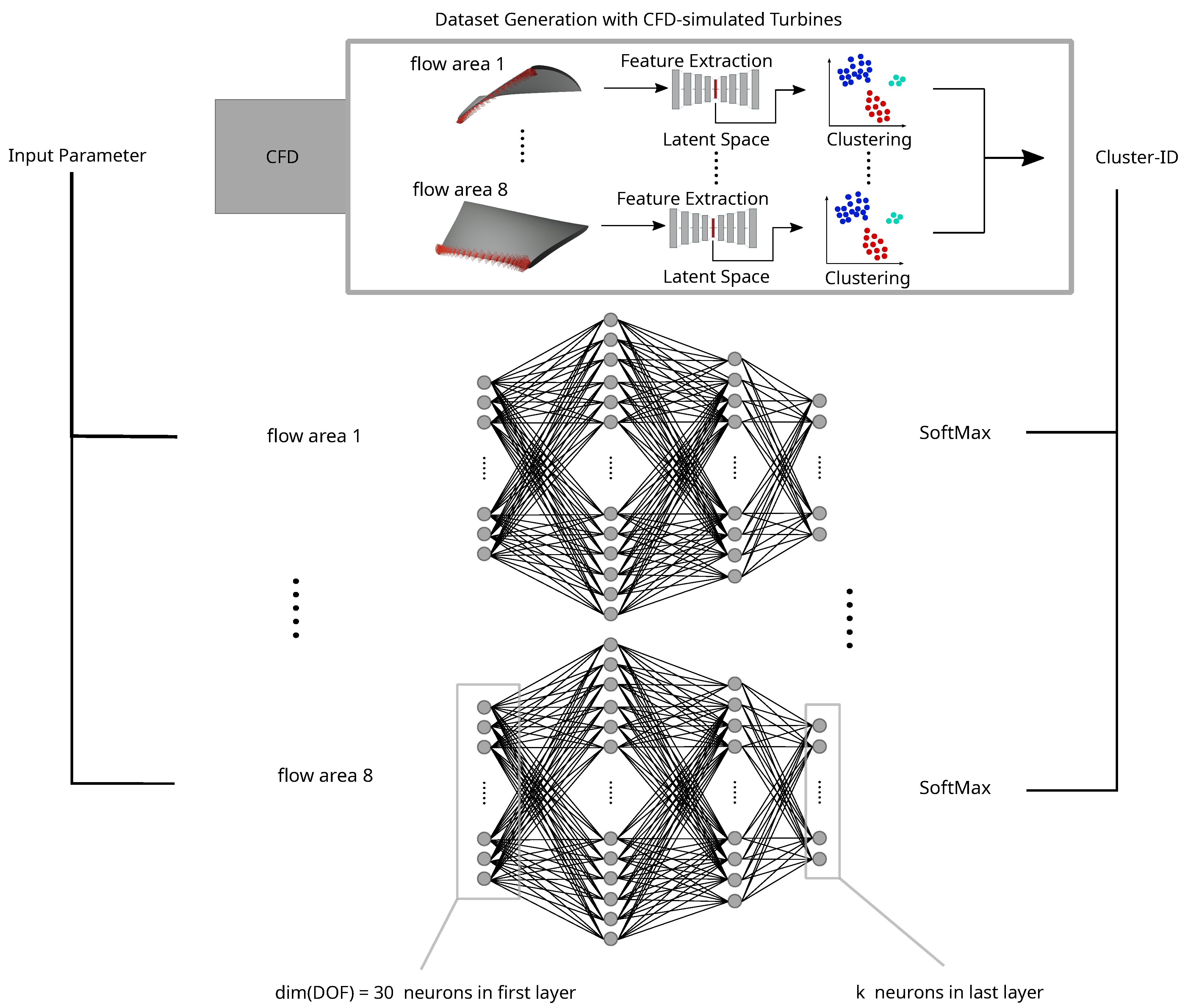
3.5. Mapping of CIs Using an NN

A multi-class prediction NN is implemented to predict the turbine’s CI prior to performing the CFD simulation. It contains one NN for each FA. The inputs of the NN are the DOFs that vary the geometry parameter. The network is then trained to predict the CI. Figure 8 shows two NNs in the center part. Each NN contains two hidden layers with 64 and 54 neurons using ReLu activation functions, respectively. The first and last layers are defined by the number of DOFs and k, respectively. The new simulated turbines are added to the training dataset to update the NNs during the optimization run. The NNs predict the CI immediately after the optimization algorithm suggests a new candidate. The predicted CI approximates the flow field for the turbine, which has not yet been simulated. This enables the evaluation of the turbine’s properties without performing a CFD simulation.

The NNs are implemented by the MLP-Classifier integrated into the scikit-learn toolbox for Python. The lbfgs solver optimizes the NN’s weights until the desired tolerance is achieved through the log-loss. As training data, 90% of turbines are used; for validation, the rest of the turbines are used. Applying the softmax function to the last layer determines the probabilities for each cluster. The cluster with the highest probability is chosen as a prediction.

Table 2. NN training parameters.

Training Data	Validation Data	Learning Rate	Tolerance Target	Optimizer
$90\%$	$10\%$	0.001	0.0001	lbfgs

summarizes the parameters for the setup of the NNs.

3.6. Integration of CIs into Optimization Process

The results in Section 3.4 show that the CI, combined with the trained NNs, approximates the turbine’s fitness values. For every new candidate, suggested by the optimization algorithm, the NN first predicts the CI. This is visualized in Figure 8 with the black lines connecting the input parameters and the NNs on the left side. The fitness approximation is initially calculated as the mean fitness value of all candidates with equal CIs. 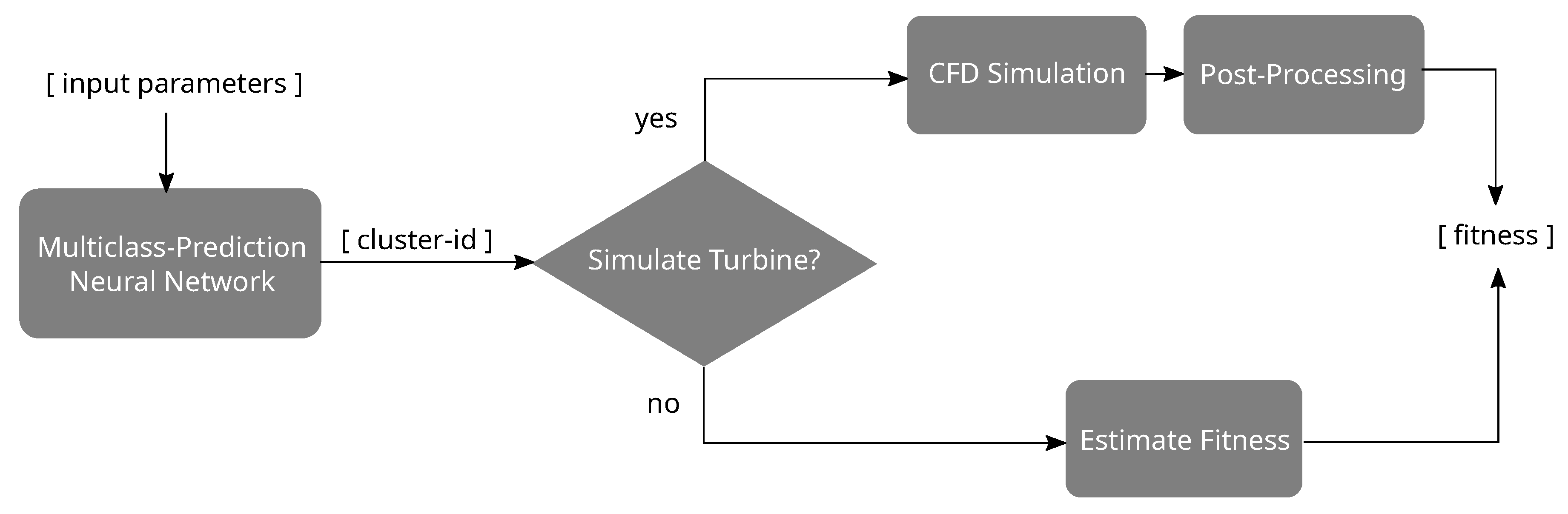For CIs with mean fitness values above a certain threshold, the candidate’s fitness value is not simulated but estimated by the design assistant. Figure 9 illustrates the structure of the design assistant.

Before a more extended optimization with the adapted optimization algorithm is run, the design assistant’s performance, depending on k, is investigated. Two different threshold-based approaches are used to decide whether to simulate the turbine or not (decision “Simulate Turbine?” in Figure 9). In the first approach, a candidate is simulated if the approximated ${\eta }_n$ is above the 50% quantile of the initial training dataset for the clustering procedure. If not, the design assistant approximates the candidate’s fitness values. This approach is used to investigate the design assistant’s performance. In the second approach, the threshold is based on the candidates during the optimization and, in that sense, dynamically adjusted during the run. The weighted sum $\overline{\eta }$ for all operating points is used here. The design assistant estimates all turbines with a predicted fitness $f\left(\overline{\eta }\right)$ value above the 40% quantile of the last 250 turbines. During the more extended optimization run, this approach is used to adapt to the latest optimized turbines’ fitness values. (Note: $f\left(\overline{\eta }\right)=1-\overline{\eta }$.)

Two different approaches for fitness prediction are compared to investigate the design assistant’s prediction performance before running a more extended optimization. The first approach estimates the fitness values by calculating the mean fitness values of the candidates with equal CIs. In the second approach, the fitness estimation is extended by a GPR using all turbines of the same CI as training data. The turbine blade’s DOFs serve as inputs for the GPR. Since the number of turbines with equal CIs might be small and the number of DOFs is very high, Principal Component Analysis (PCA) reduces the dimension of the DOFs. Within the GPR, a Radial Basis Function Kernel is used for the covariance functions. In both approaches, the candidate’s fitness is simulated if the NN predicts a CI that has not occurred before.

4. Results

To investigate the design assistant’s prediction performance dependent on k, an optimization with NSGA-II is used, applying an island model with ten islands. Within the first investigation, the influence of k = 16 and k = 20 on the results is investigated with a focus on the Spectral Clustering algorithm. The first 1000 candidates are simulated conventionally and used as initialization for the adapted optimization and for the design assistant. The optimization of the next 1000 individuals is performed with the adapted optimization algorithm. The prediction accuracy of the design assistant is evaluated by resimulating the previously approximated candidates.

Table 3. Fitness deviation of the first 100 predicted turbines for different values of k and with or without GPR for fitness value approximation.

Prediction Deviation	Deviation Fitness $\mathit{f}\left(\overline{\mathit{\eta }}\right)$ [%]	Deviation Fitness Cavitation Volume $\overline{{\mathit{V}}_{\mathit{cav}}}$ [l]
k = 16	0.32	0.38
k = 16 with GPR	0.28	0.44
k = 20	0.495	0.54
k = 20 with GPR	0.29	0.25

displays the deviations for the fitness prediction depending on k and GPR. GPR is only used if at least two different individuals share the same CI. Even with the integration of GPR, some fitness values are still predicted by the CI’s mean fitness values if there is not more than one different turbine sharing that CI. The overall best performance delivers k = 20 with the use of GPR. This configuration is used for the more extended optimization run.

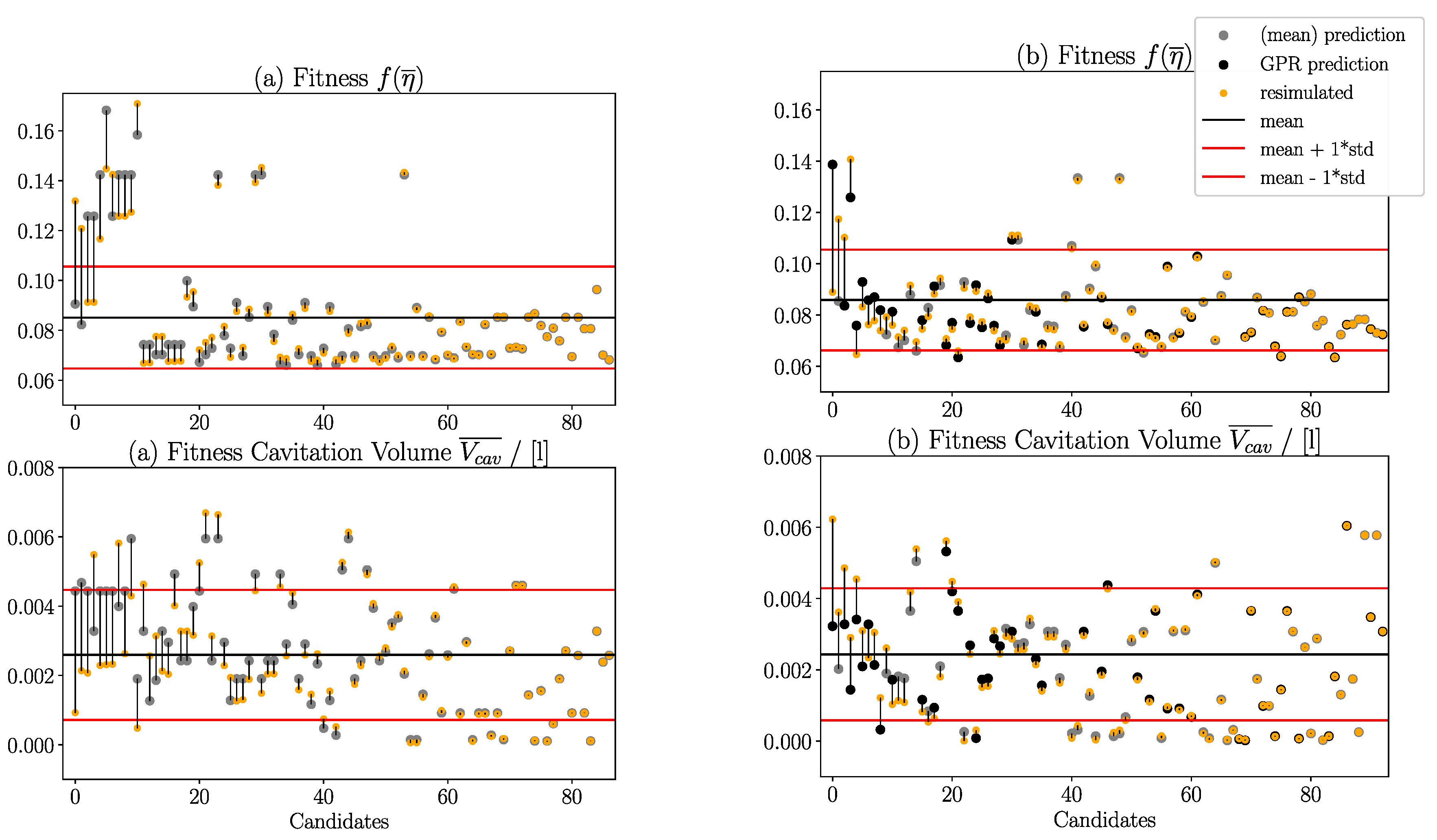
Figure 10 shows the difference between the approximated and simulated fitness values for k = 20 with and without the use of GPR. The mean and standard deviation of the complete database’s fitness $f\left(\overline{\eta }\right)$ values are shown as black and red lines. Estimated turbines might turn out to be pumps instead of turbines, or their head deviation might exceed a permissible value. In this case, they are assigned with a “failed” fitness and not pictured in Figure 10. This phenomenon is discussed later in Section 5 of this work.

Before the more extended optimization starts, each of the design assistant’s AEs is pretrained by the initialization dataset. After each tenth generation on the first island, the AEs are retrained by the updated database. The NNs for CI prediction are also retrained after every tenth generation on each island. The same initialization dataset is used as for the performance investigation. This time, the dynamically adapted threshold for the simulation decision is used. Every CI with an expected fitness $f\left(\overline{\eta }\right)$ above the 40% quantile of the last 250 candidates is not simulated but estimated by the design assistant.

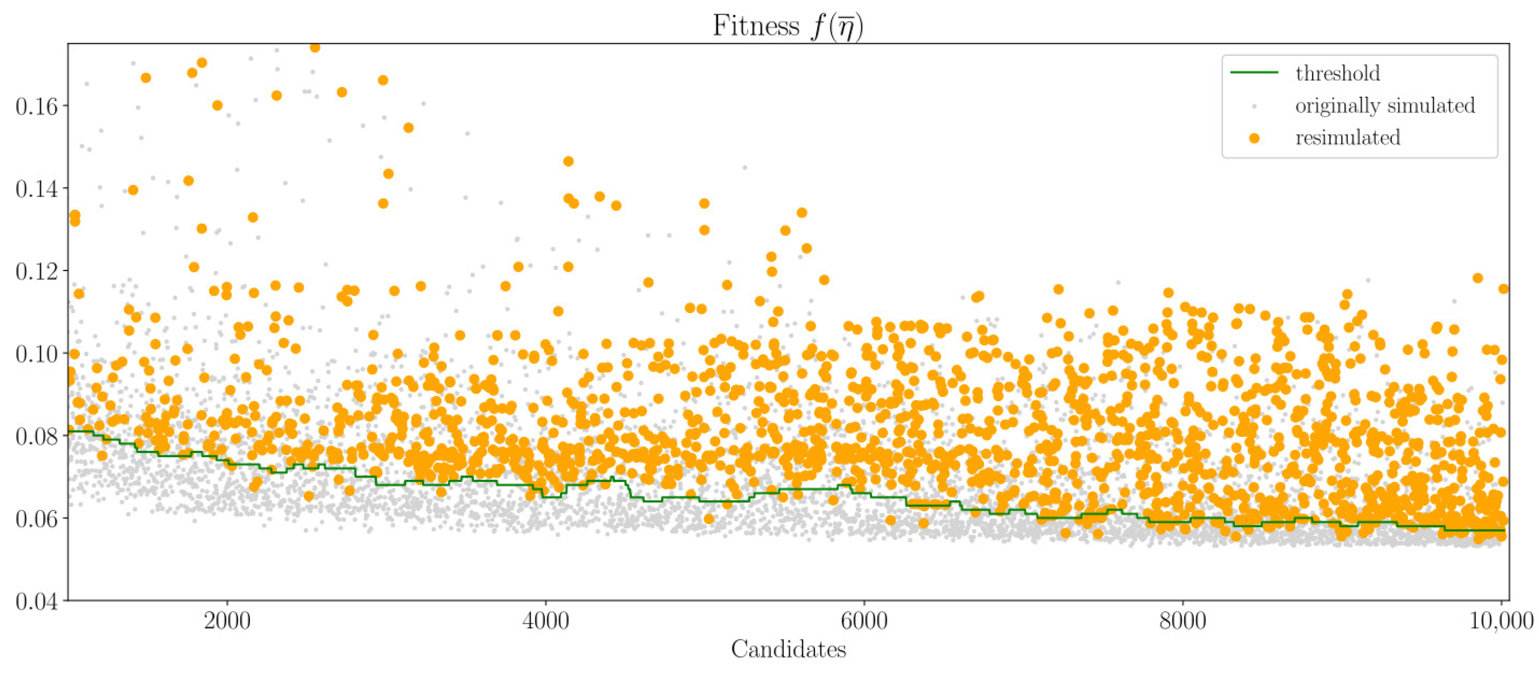
Each island runs its own computing process, and, therefore, each island runs its own design assistant’s Python object. The optimization process runs asynchronously on each island. As a result, the retraining of the NNs and the threshold adjustment run asynchronously for each island, even if the objects of the design assistant share the same database. Figure 11 shows the resimulated fitness values of the previously estimated turbines during the optimization run. The turbines’ fitness values are sorted by their chronological occurrence. The green line marks the 40% quantile threshold. The target of the design assistant is to keep the resimulated turbines’ fitness $f\left(\overline{\eta }\right)$ above the threshold line.

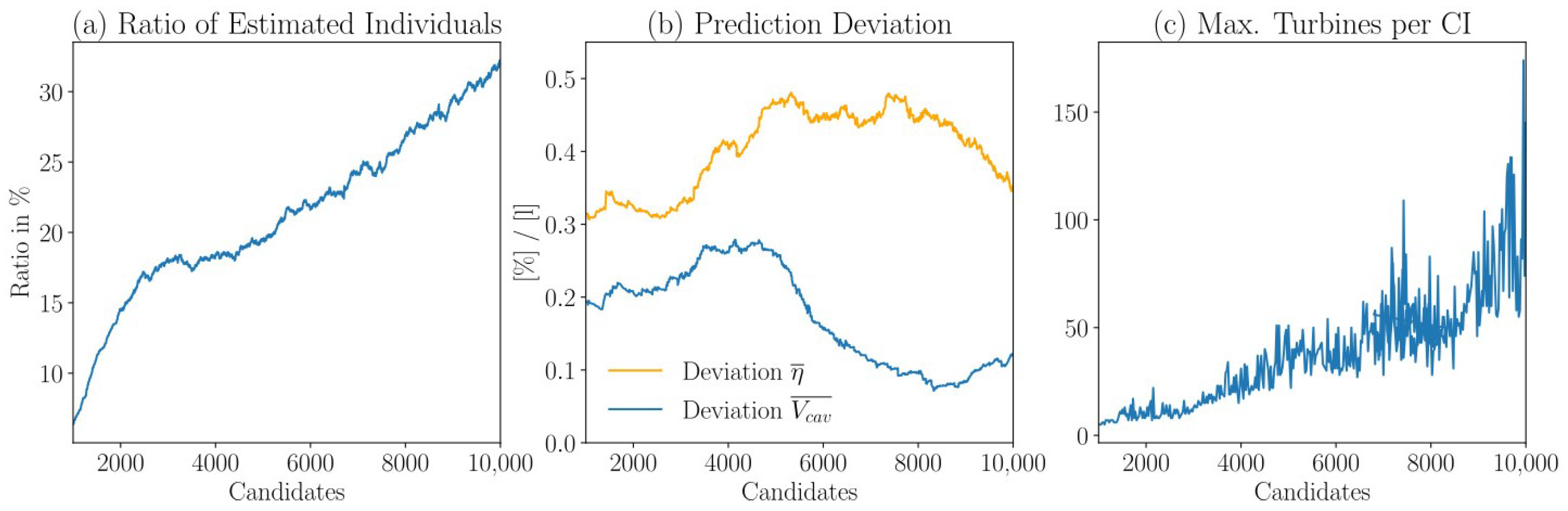
Figure 12a illustrates the current ratio of the turbines estimated by the design assistant to the turbines suggested by NSGA-II along the optimization process. With the ongoing optimization, the design assistant’s database contains more turbines. Therefore, more CIs are already known by the design assistant. Consequently, fewer CIs predicted by the NNs are unknown and must, thus, be simulated using CFD and the ratio of estimated turbines increases.

Figure 12b illustrates the prediction deviation, both for fitness $f\left(\overline{\eta }\right)$ and for the cavitation volume $\overline{V_{cav}}$. While the prediction deviation initially increases, a decrease is noticeable after 5000 candidates, especially for the cavitation volume.

Figure 12c shows the maximum number of turbines sharing the same CI during the course of the optimization. In all three figures, the x-axis displays the optimization course for the turbines proposed by NSGA-II.

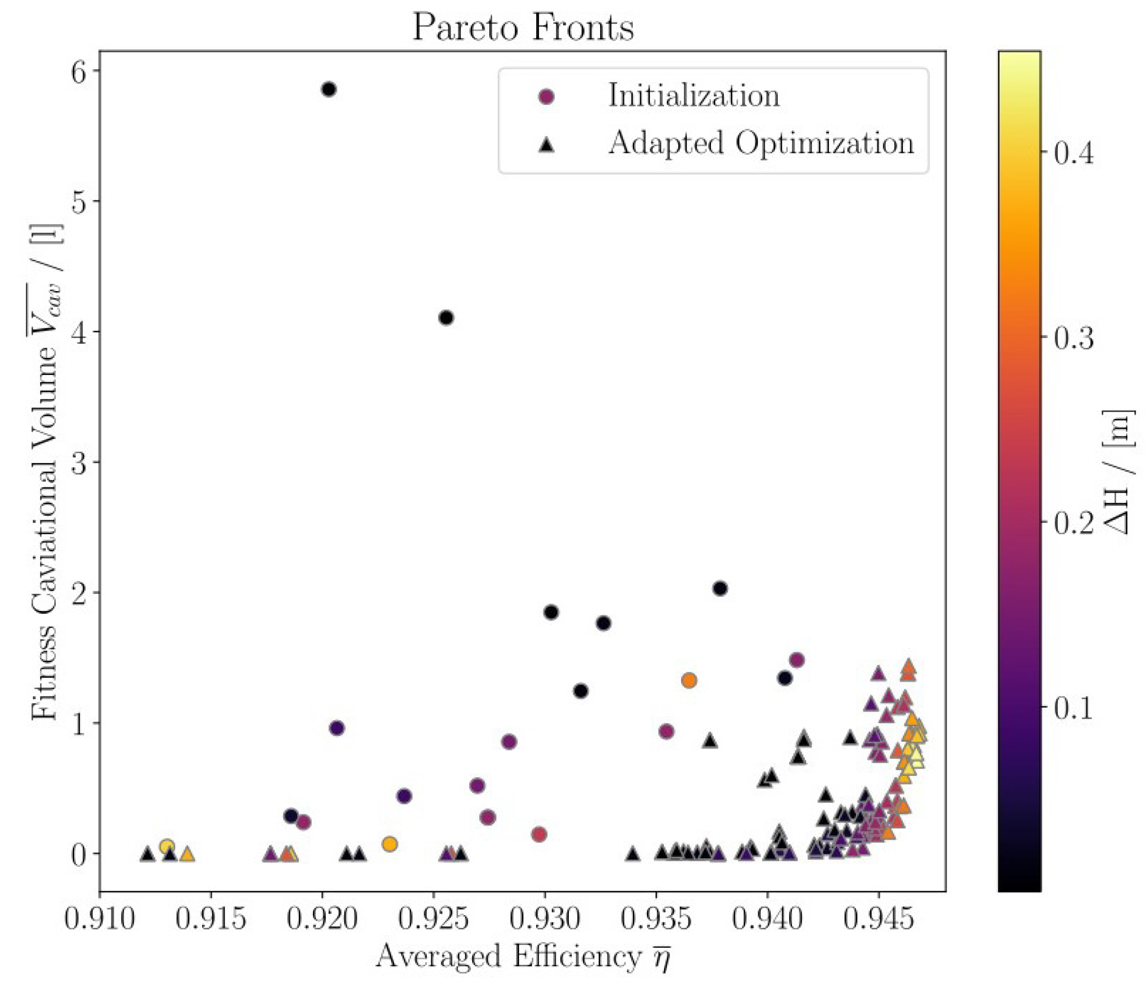
Figure 13 presents the optimization’s Pareto front. The dots mark the initialization dataset. The triangles mark the latest Pareto front of the optimization adjusted by the design assistant. During optimization, turbines with high efficiency are found, while retaining a low cavitation volume. Since the head was an optimization constraint, the head deviation to the desired target value is represented by the color bar.

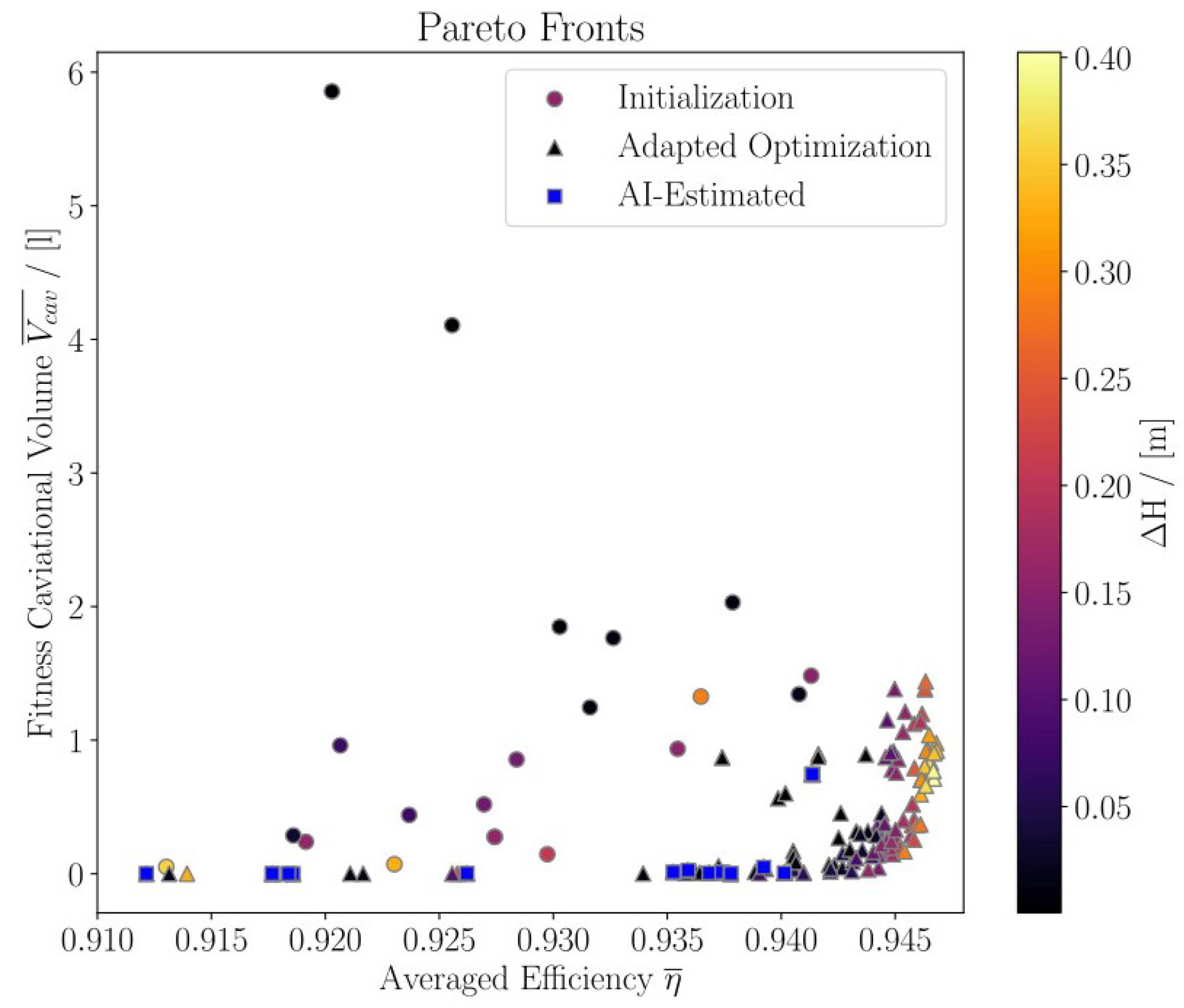
As shown in Figure 14, low-efficiency individuals that were previously estimated turn out to be part of the final Pareto front. These turbines were never CFD-simulated and stayed in the first Pareto front during the optimization.

5. Discussion

The optimization of hydraulic machinery is a high-dimensional optimization task that requires a high number of CFD simulations. While this work’s axial turbine test case contains 30 DOFs, “real-world” machinery might be even more complex. This work provides an approach to reduce the number of function evaluations during optimization. While conventional optimization using EAs does not use the CFD-generated flow fields other than for computing fitness values, the clustering approach evaluates flow field data, gaining additional information. This information is used to accelerate the optimization process. The results in Section 4 show that the AEs, combined with the Spectral Clustering algorithm, can cluster three-dimensional flow fields of an axial turbine test case into groups with similar fitness properties. This is achieved by dividing the flow fields into FAs. By employing NNs to predict a turbine’s CI, the assignment of a turbine to its cluster group can be predicted without applying CFD simulation. In combination with GPR, the fitness values of turbines can be predicted and integrated into an adapted optimization process based on NSGA-II. Resimulating estimated turbines shows that the design assistant can identify turbines with low efficiency without CFD simulation, as shown in Figure 11. Figure 13 shows that the adapted optimization algorithm creates an advancing Pareto front. Turbines with high efficiency and low cavitation are found during the optimization. By integrating the design assistant into NSGA-II, turbines expected to have unwanted flow fields are estimated. This approach leads to a reduction inCFD simulations of over 20%.

NSGA-II strives to resolve the complete Pareto front [32]. This results in a high diversity of turbines included in the Pareto front. Therefore, NSGA-II finds turbines with high efficiency and high cavitation and turbines with low cavitation and low efficiency. By employing the design assistant, it is possible to estimate turbines in fitness regions of low interest, e.g., high-cavitation turbines. Computational resources can be focused on other fitness regions. The impact of the estimated turbines on the convergence of the adapted optimization remains unclear. Due to the stochastic approach of NSGA-II, not much information is gathered by comparing just two different optimization runs. To receive unambiguous information, several optimization runs must be carried out for both: the accelerated and the conventional run. This goes hand in hand with high computational cost and is not performed here.

Figure 10 describes the prediction performance of the first 100 estimated turbines. The design assistant could estimate a turbine during the optimization process whose CFD resimulation delivers “failed” fitness values. “Failed” fitness refers to artificially high fitness values generated mainly by a penalty function. These occur in cases where the CFD simulation diverges, the head deviation exceeds a permissible limit, or a pump is detected instead of a turbine. These cases are not covered by the design assistant, since it does not receive their flow fields for clustering. This can result in a bad prediction accuracy for several candidates. While investigating the prediction accuracy for 100 estimated turbines, this occurred for k = 20 seven times with GPR and three times without GPR. For k = 16, it happened six times with GPR and four times without GPR. Diverged CFD simulations are not taken into account here. Although this effect might depend on the decision for or against GPR, this cannot be the case. As soon as the design assistant chooses to estimate a turbine’s fitness values, this turbine is assigned with fitness values determined based on CFD-simulated turbines with the same CI. Since the design assistant does not process turbines’ flow fields with “failed” fitness values, these fitness values are not contained in the database. Therefore, candidates with “failed” fitness values should not be chosen for estimation by the design assistant. Nevertheless, this happens during the optimization and is a topic for future research. Since failed fitness values are artificially high, these are not investigated when comparing the prediction accuracy between different k values and are not pictured in Figure 10. This is because artificially high fitness values distort the accuracy mean.

The design assistant can estimate turbines in specific fitness regions. This leads to candidates contained by the Pareto front that are not CFD-simulated. This behavior is illustrated in Figure 14. These individuals can be part of their island’s population from the moment they are estimated. It is expected that these turbines will have low efficiency values as a result of the introduced estimation threshold. The effect of estimated candidates staying on an island’s population during the optimization remains unclear and might be further investigated. Since actual and AI-generated fitness values are not distinguished, NSGA-II treats both cases equally. This property leaves room for further adaption and future research in integrating AI-generated fitness values into the optimization process.

Figure 12 shows the design assistant’s behavior changing the increasing size of the data. The prediction accuracy varies with the changing amount of data. A clear pattern is not noticeable. The fitness prediction works as a two-step process. First, the prediction of the CI by NNs is made, and, subsequently, the fitness prediction based on CFD-simulated turbines sharing the predicted CI is executed. Both processes impact the prediction accuracy. Applying GPR enables the automatic interpolation of fitness values in well-investigated areas of DOF space while relying on prior assumptions in less-known areas of design space. Still, the choice of dimension for this interpolation by pre-processing using PCA and GPR parameter determination influences fitness prediction. This shows that several parameter choices regarding prediction accuracy are still to be investigated. Additionally, determining the optimal value of k is ambiguous and may depend on the database size. The decision for k must be made by the user immediately. During optimization, the database size changes continuously, impacting the clustering results, as shown in Figure 12c. The choice of k must be examined more closely in future applications of the design assistant. The optimal choice of k might vary for each of the FAs. As a result of the growing database size, the choice of k must be automated to adapt to changing conditions by itself. Potentially interesting criteria for an optimal choice of k provide scope for future investigations. Outliers in clustering and their role in prediction can additionally be investigated. The clustering’s distribution of turbines into groups of the same CI should avoid outliers with different flow properties. This is because outliers can distort the predicted fitness values mistakenly. So, the detection and removal or even prevention of outliers might be beneficial for prediction accuracy and future algorithm improvement.

Each turbine’s flow field is divided into eight FAs. The authors believe that having an equal number of FAs at the high-pressure side and low-pressure side benefits clustering. Therefore, the choice for the number of FAs must be an even number. A higher number might resolve flow field properties more accurately, leading to CIs that contain more digits. More NNs will be required to predict the CI with a higher number of FAs. This might lead to inaccuracies in predicting the correct CI, since more digits have to be correctly determined. Additionally, higher computational costs regarding feature extraction, clustering, and prediction occur, since more AEs and NNs are required. A lower number of FAs leads to a coarser resolution of the flow field and might reduce clustering quality, especially for growing database sizes. FewerAEs are required for feature extraction and fewerNNs for CI prediction. This might lead to fewer prediction inaccuracies and lower computational cost. Considering this, the authors chose to work with eight FAs for their investigations.

The ratio of bypassed CFD simulations estimated by the design assistant rises above $30\%$ during optimization. This shows the design assistant’s potential to reduce the number of function evaluations significantly. Nevertheless, this ratio is only achieved after many function evaluations. The ability to predict more turbines from the beginning of the optimization has not yet been achieved, since there are limited amount of data. Integrating information from other hydraulic machinery into the design assistant’s database is an area for future research. This enables the integration of pretrained AI models in the optimization process to increase prediction accuracy and database size independently of the ongoing optimization.

6. Conclusions

This work presents an innovative approach to evaluate axial turbine fitness properties without relying solely on computationally expensive CFD simulation. Employing a clustering-based design assistant, the method significantly reduces the computational burden typically associated with turbine design optimization. CFD simulation of low-efficiency candidates can be avoided, while the influence of AI-estimated turbines on convergence remains to be investigated in the future. The clustering-based approach leverages AEs followed by Spectral Clustering techniques to analyze and group similar flow field patterns around axial turbines. This method allows for rapid assessment of turbine performance characteristics, offering a more efficient alternative to traditional CFD simulations. In combination with NSGA-II, an adapted optimization algorithm is introduced. This hybrid approach integrates the clustering-based fitness evaluation with the multi-objective optimization capability of NSGA-II, enabling a more efficient design space exploration. The optimization results provide the following insights:

• The design assistant predicts turbines’ fitness values with a reasonable accuracy and can group turbines of similar flows.
• Even with a dataset of fewer than 1000 turbines, the design assistant can identify similar flow fields and predict fitness values without performing a CFD simulation.
• The adapted algorithm can identify turbines with bad fitness values and avoid timeconsuming simulations of those turbines. With ongoing optimization, the ratio of currently estimated individuals rises above $30\%$.
• During optimization, 9000 individuals are evaluated. The adapted optimization algorithm estimates $21.4\%$ of these. Since the computational effort of training the AI-based design assistant is negligible, around $20\%$ of computational resources are saved by integrating the design assistant into the optimization process.
• The adapted optimization algorithm finds high-efficiency and low-cavitation individuals, which dominate the initialization individuals. An advancing Pareto front is created.

The design assistant’s ability to bypass CFD simulations for specific fitness regions is instrumental (see Figure 11). The threshold between simulating or estimating individuals is freely determinable. It is possible to specify attributes of turbines that should not be simulated. This enables focusing more on interesting fitness regions during optimization and using estimations in other fitness regions. This feature enables more control over computational resources in high-dimensional and multi-objective optimization, allowing for a more targeted use of CFD simulation.

For future research, it is desired to extend the design assistant’s capability to group flow fields for more than one test case simultaneously. Performing flow field clustering for different test cases simultaneously enables the possibility of growing a database to pretrain the design assistant even before the optimization. Figure 12a illustrates the rising ratio of estimated turbines with increasing database size. Consequently, running the pretrained design assistant would bypass more CFD simulations. The determination of k should further be investigated and automated to adapt to different dataset sizes and populations.