Modelling and Transient Simulation of District Heating Networks Based on a Control Theory Approach ^†

Abstract

Heating districts have become one of the key infrastructures to efficiently and sustainably supply heat to consumers. With the current climate change crisis, not only are heating districts of the essence but their efficient and optimized operation as well. To analyze and achieve such an optimization, transient simulations of heating districts are needed. These simulations are a means of upgrading older town networks to smarter energy grids as well as an effective tool for the planning and building of newer heating networks. Therefore, this work presents an easy simulation method for the transient simulation of heating districts based on a control theory approach. The simulation method can calculate multiple-loop networks as well as non-looped networks and correctly predict how a heating network can behave over time. Additionally, this approach allows for the inclusion of new renewable energy sources into existing heating networks and to simulate the resulting network behavior. The method was tested on five different testcases involving a single-loop network, a multiple-loop network, and a real-life non-looped network. In each case, the calculated massflows were validated with the software Epanet (Version 2.2), while the simulated temperatures were compared to the theoretical steady-state values as well as the theoretical times of arrival of each heating network. The simulation results present a good approximation in each testcase. Finally, the limitations of the method are discussed, and a recommendation for the usage of the approach is given.

1. Introduction

In tackling the current climate change crisis, district heating networks have gained particular importance. Their ability to efficiently supply private households, commercial units, and heavy industry with heating places them as one of the most important key infrastructures in modern city planning and supply management. In this context, the adaptations of older energy grids as well as the optimization of current working city networks are the main focus of state-of-the-art research. A modern heating district network usually consists of a feed line, which transports a heated medium to customers, and a return line, which transports the cooled medium back to its source. Sources are either centralized power plants like CCGT (combined cycle gas turbine) plants or decentralized power plants like solar thermal collectors. The current modernization of older heating district networks tends to include more decentralized suppliers as well as a general temperature reduction in the feed and return line. For this reason, simulations of district heating networks are considered a state-of-the-art procedure and are nearly always included in every city planning or modernization project. However, current simulations of district heating networks are often limited to steady-state solutions and negate the transient behavior of these systems. In the past, this was sufficient for monitoring or regulation processes due to interest in the sole steady-state solution. The more modern and decentralized plants, however, demand higher flexibility of the networks, which is often negated in these steady-state solutions. With the increasing complexity of these heating networks and more decentralized supplier and consumer behaviors, transient simulations are needed.This is work is an extended version of our paper published in the 19th Conference on Sustainable Development of Energy Water and Environment Systems [1].

There already exist various simulation models for the transient simulation of district heating networks, such as the works [2,3,4,5,6,7,8,9,10,11,12,13,14,15,16,17,18,19]. Although these works can be considered as state of the art for transient simulations of heating districts, sometimes their transparency and reproducibility are limited. Additionally, there seems to be two main issues regarding the transient simulations of district heating networks. The first issue is the correct calculation of the massflow distribution in a looped heating network. The second issue is the actual transient simulation and numerical simulation as well as the computational workload they usually demand. Therefore, solutions for these issues tend to vary significantly, from very detailed one-dimensional CFD simulations of heating networks to simplified lumped heat models for the calculation of larger heating grids. Ref. [2] created a transient simulation tool for district heating with a primal focus on lag times and attenuation degrees of district heating systems. Their calculation relies on a space- and time-dependent differential equation, which was tested on three simple but different district heating networks. One of their main assumptions is that the flow rate is kept constant. Ref. [3] created a prediction method for the simulation of thermal transients in district heating systems. Similarly to [2], they used a space- and time-dependent differential equation for the calculation of thermal transients. They used a steady-state hydraulic solution for the pressure changes and massflows within the heating network. Their tested network does not have internal loops. Ref. [4] tested two different transient simulation approaches (TERMIS software and a node method) on their measured district heating system. Their measured system has no internal loops. Similar to ref. [4], ref. [5] tested a software (AMBASSADOR) for the simulation of transient district heating behavior. The software is a framework in Modelica and is a library for detailed models of the distribution and consumption components found in district heating systems. The tested software was compared to two different types of software (IDA-ICE and Apros). Ref. [6] presents a transient simulation model (ISENA) that calculates a quasistatic hydraulic model and a transient thermal model for district heating networks. Their quasistatic hydraulic model calculates the massflows occurring in a heating network, which are input needed for the calculation of the transient temperatures in their thermal model. Their model seems to include the calculation of network loops. Ref. [7] focuses on the simulation of bidirectional power flows in district heating networks. Their work derives a holistic mathematical system for the calculation and regulation of the network’s thermohydraulic steady state. Their networks include multiple internal loops. The simulation method focuses only on the steady state. Ref. [8] presented a new software implementation within the IBPSA Modelica Library for the transient simulation of thermohydraulic district heating networks. Their model focuses on the transient calculation of the massflow change and the temperature change in a district heating network. The presented heating network has no interacting loops. Ref. [9] deals with the full transient simulation of district heating networks, including massflow change and looped networks. The focus of the work was to study the effects of network dynamics in contrast to steady-state solutions. Ref. [10] focuses on an alternative formulation of the Global Gradient Algorithm (GGA) for the correct calculation of massflow in a multiple-loop network. The algorithm includes the calculation of nonlinear pressure terms in looped systems but not the calculation of the transient temperature changes in a network. Ref. [11] presents a simulation method in Matlab/Simulink for the correct calculation of the massflows inside a looped network and the analyzation of the resulting temperature distribution. Their work focuses on the steady-state behavior of networks. Ref. [12] compares two open-source approaches (DHNx/SESMG and Thermos) for the modeling and optimal integration of heating networks. Their focus is the optimization of heating networks. Ref. [13] uses a new one-dimensional finite-volume method to simulate approximated heat wave propagations inside heating networks. Their work focuses on the correct transient simulation of heat waves propagating throughout a test network including a turbulence model and correct numerical stability. The work, however, does not clarify if the tested network has internal loops. Ref. [14] presents a new alternative adjoint-based numerical optimization strategy for the simulation of large-scale nonlinear thermal networks. Their focus is on the optimization of network topology and pipe size diameters on large-scale networks. The presented heating districts involve multiple-loop networks as well as independent suppliers and consumers. Ref. [15] deals with a systematic approach of simplifying heating network topology complexity for the purpose of reducing the computational workload caused by the transient simulations. Their network topology does not include loops. Ref. [16] presents an equivalent model for the dynamic simulation of combined district heating networks and electricity operations. Their main focus lies in the optimization of both combined systems. Ref. [17] focuses on the technical–economical optimization of district heating networks. Their tested network has no loops. Ref. [19] presents a new transient and multiple-timescale simulation method for the calculation of combined electricity and heating networks. They use a space- and time-dependent formulation for heat wave propagation. Their tested heating network has no internal loops. Ref. [20] created a data-based compact model or reduced-order model for the prediction of transient temperature evolution in a district heating network. They assume throughout the simulation time a constant massflow inside the pipes, and their tested network has no interacting loops.

In summary, the transient simulation of district heating networks usually includes multiple space- and time-dependent differential equations of the heat wave propagation. However, for the fully correct numerical simulation of a heat wave propagation, not only do the transient temperature changes have to be calculated but also the transient massflow change inside a network. This nearly always results in a full one-dimensional CFD simulation of a pipe flow. Unfortunately, these kinds of calculations demand, under normal circumstances, a high amount of computational workload and are limited for large-scale networks. Secondly, the correct massflow calculations inside a looped network tend to have numerical issues when included in a one-dimensional CFD pipe flow. This is the reason why most simulation models focus either on single-branch networks or use a simplified simulation approach for calculations of larger multiple-loop networks. Thus, this work aims to provide an easy-to-implement and simplified simulation method for the transient simulation of looped and non-looped district heating networks.

2. Materials and Methods

As presented before, there are many various ways to calculate the transient behavior of district heating networks. This paper presents an approach based on control theory, which can be considered as an easy-to-understand method that is more easily implemented for the simulation of transient district heating networks. A simulation approach based on control theory is one where every time-dependent temperature change in a network can be calculated via a state-space model as in the following equation:

$$\dot{x}=A·x\left(t\right)+B ·u\left(t\right)$$

(1)

State-space modeling is already a proven practice in many transient simulations of dynamic systems. It has found a wide range of uses from live process controlling to the simulation of house heating and the optimization of energy costs [21]. Particularly, house heating simulations have proven that, due to their similarities to district heating, state-space modeling can be used for transient simulations of district heating networks.

However, to use state-space modeling for transient simulations of heating networks, certain steps need to be taken. The final model itself consists of three different smaller mathematical models or matrices, which in summation allow the state-space modeling of the heating networks and thus the simulation of the transient behavior. As mentioned before, there are two main issues regarding the simulations of heating networks. The first one is the correct calculation of the massflow distribution in a looped network. Looped networks in general are heating networks where one or usually more pipe loops are present. These loops cause a different pressure distribution inside a heating network and result in a different massflow distribution than in a simple non-looped network. Therefore, the first smaller model of this work focuses on the correct massflow calculation in a looped network and is called a “hydraulic model”. With known massflows in every pipe, the second smaller so-called “thermodynamic model” converts the massflow information into a mathematical description of the thermodynamics-dependent network. Finally, the “comprehensive model” uses the information of every other model to create the state-space modeling of the heating network and simulates the transient behavior. In this context, the first issue of transient simulations of heating networks is being solved by the hydraulic model, wherein the second issue regarding the numerical simulations is being solved in the thermodynamics and comprehensive model. In the following, every model will be explained in more detail.

2.1. Hydraulic Model

The hydraulic model uses the characteristics and structures introduced in graph theory for the mathematical description of a heating network. Simplified, the graph theory uses so-called nodes and edges to describe a network. Applied to a heating network this means that edges are pipes, while nodes are usually every pipe connection, every supplier (source) and every consumer (sink). With the help of the graph theory the very massflow distribution in a non-looped or looped network can be calculated. While there are better algorithms to calculate the massflow distribution in a network, like the “Global Gradient Algorithm” used by the software Epanet [10], this work focuses on an older numerical approach by Chua [22] to calculate the massflow distribution in every pipe. The reason why this work uses the older approach by Chua is that it is fundamentally easier to implement in a program and easier to find potential issues in the numerical solution. Mathematically the algorithm by Chua works by the same principle as more modern approaches like the Global Gradient Algorithm. Additionally, Chua’s algorithm was originally developed for electrical circuits but can be adapted for the calculation in heating networks due to the similarities between electrical and hydraulic networks

The purpose of the hydraulic model is to calculate the massflows of every pipe. Due to the difficulties of looped networks massflow calculations tend to be quite complex, nearly always resulting in a numerical solution of a system of equations. In essence, the calculations of the hydraulic model can be divided into two different approaches. The first approach focuses on non-looped networks or simplistic heating networks, wherein the heating network only consists of single branches and no interacting loops. The second approach deals with complex heating networks, where one or more loops are interacting with the massflow distribution. Figure 1 presents a visual description of a simplistic and complex heating network.

The hydraulic model solves both types of networks with the following equation:

$$M_{hyd}·{\dot{m}}_{unkown}={\dot{m}}_{Sources}$$

(2)

${\dot{\mathit{m}}}_{\mathit{u}\mathit{n}\mathit{k}\mathit{o}\mathit{w}\mathit{n}}$ are the unknown massflows of the networks, which occur in Figure 1 inside the pipes a to d. ${\dot{\mathit{m}}}_{\mathit{S}\mathit{o}\mathit{u}\mathit{r}\mathit{c}\mathit{e}\mathit{s}}$ are the known massflow sources and sinks or junctions inside the network represented as Nodes A to F. ${\mathit{M}}_{\mathit{h}\mathit{y}\mathit{d}}$ is the hydraulic model, which connects the full system of equations and makes it ultimately solvable for a numerical solver. The approach for the solution of both network types differs in the creation of the ${\mathit{M}}_{\mathit{h}\mathit{y}\mathit{d}}$ matrix. For simplistic heating networks the ${\mathit{M}}_{\mathit{h}\mathit{y}\mathit{d}}$ only consists of the incidence matric “${\mathit{A}}_{\mathit{i}\mathit{n}\mathit{c}\mathit{i}}$” of the network and can be easily solved with a simple solver for system of equations like the Gaussian Elimination Method. For complex networks, where one or more loops are present, the second approach via the algorithm of Chua is used [22]. The mathematical reason why both approaches are used is in the composition of the ${\mathit{M}}_{\mathit{h}\mathit{y}\mathit{d}}$ matrix. For simplistic networks the system of equations has a greater number of equations to unknown parameters, which can be easily solved by standard solvers. In case of a complex network the system of equations has either the same amount or less equations needed for the unknown parameters. On top, these systems of equations are linear-dependent, making them difficult to solve for standard solvers. The algorithm by Chua [22] considers both issues and converts the standard hydraulic matrix into a linear independent matrix, which then can be solved via a numerical solver.

In the following the algorithm by Chua [22] is applied on a heating network. The usual approach by the algorithm uses the incidence matrix ${\mathit{A}}_{\mathit{i}\mathit{n}\mathit{c}\mathit{i}}$ of a network to calculate a cutset matrix “D” and resulting in a loop or tieset matrix “${\mathit{B}}_{\mathit{l}\mathit{o}\mathit{o}\mathit{p}}$”. With a known incidence matrix and loop matrix the full hydraulic model for complex networks can be created

$$M_{hyd}=\left[\begin{array}{c}{A}_{new}\\ B_{new}\end{array}\right]$$

(3)

${\mathit{A}}_{\mathit{n}\mathit{e}\mathit{w}}$ and ${\mathit{B}}_{\mathit{n}\mathit{e}\mathit{w}}$ are adjusted incidence and loop matrices. The ${\mathit{A}}_{\mathit{n}\mathit{e}\mathit{w}}$ is the arbitrarily shortened incidence matrix ${\mathit{A}}_{\mathit{i}\mathit{n}\mathit{c}\mathit{i}}$ as explained in [22]. The ${\mathit{B}}_{\mathit{n}\mathit{e}\mathit{w}}$ matrix needs to be an updated loop matrix with the friction coefficient of the calculated pipes in the loop matrix. The ${\mathit{B}}_{\mathit{l}\mathit{o}\mathit{o}\mathit{p}}$ matrix can be updated following equations [23]:

$$B_{new}=B_{loop}·K ·\left|{\dot{m}}_{unkown}\right|$$

(4)

With K as the resistance coefficient of the specific pipe [24]:

$$K={\displaystyle \frac{8 ·L·f}{D^5·{\rho }^2{·\pi }^2·g}}$$

(5)

L is the specific pipe length, f is the friction factor, D is the pipe diameter, $\mathit{\rho }$ the density of water and $\mathit{g}$ is the gravitational force of the earth. The complex hydraulic model ${\mathit{M}}_{\mathit{h}\mathit{y}\mathit{d}}$ can then look like the following example:

$$M_{hyd}=\left[\begin{array}{c}{A}_{new}\\ B_{new}\end{array}\right]=\left[\begin{array}{cc}\begin{array}{ccc}\begin{array}{ccc}\begin{array}{c}-1\\ \begin{array}{c}1\\ \begin{array}{c}0\\ \begin{array}{c}0\\ \begin{array}{c}0\\ 0\end{array}\end{array}\end{array}\end{array}\end{array}& \begin{array}{c}0\\ \begin{array}{c}-1\\ \begin{array}{c}1\\ \begin{array}{c}0\\ \begin{array}{c}0\\ K_b\left|{\dot{m}}_b\right|\end{array}\end{array}\end{array}\end{array}\end{array}& \begin{array}{c}0\\ \begin{array}{c}0\\ \begin{array}{c}-1\\ \begin{array}{c}1\\ \begin{array}{c}0\\ 0\end{array}\end{array}\end{array}\end{array}\end{array}\end{array}& \begin{array}{c}0\\ \begin{array}{c}-1\\ \begin{array}{c}0\\ \begin{array}{c}0\\ \begin{array}{c}1\\ {-K}_c\left|{\dot{m}}_c\right|\end{array}\end{array}\end{array}\end{array}\end{array}& \begin{array}{c}0\\ \begin{array}{c}0\\ \begin{array}{c}0\\ \begin{array}{c}0\\ \begin{array}{c}-1\\ 0\end{array}\end{array}\end{array}\end{array}\end{array}\end{array}& \begin{array}{c}0\\ \begin{array}{c}0\\ \begin{array}{c}-1\\ \begin{array}{c}0\\ \begin{array}{c}1\\ K_d\left|{\dot{m}}_d\right|\end{array}\end{array}\end{array}\end{array}\end{array}\end{array}\right]$$

(6)

With the created hydraulic model, the unknown massflows in Equation (2) can be solved with a numerical solver for system of equations. In this work the Newton–Raphson method has been used via the following example:

$$\left[\begin{array}{c}{\dot{m}}_{unkown\left(1\right)}^{n+1}\\ ⋮\\ {\dot{m}}_{unkown\left(i\right)}^{n+1}\end{array}\right]=\left[\begin{array}{c}{\dot{m}}_{unkown\left(1\right)}^n\\ ⋮\\ {\dot{m}}_{unkown\left(i\right)}^n\end{array}\right]-{\left[J^n\right]}^{-1}·\left[\begin{array}{c}∆F\left({\dot{m}}_{unkown\left(1\right)}^n\right)\\ ⋮\\ ∆F\left({\dot{m}}_{unkown\left(i\right)}^n\right)\end{array}\right]$$

(7)

With the system of equations as follows:

$$\left[\begin{array}{c}∆F\left({\dot{m}}_{unkown\left(1\right)}^n\right)\\ ⋮\\ ∆F\left({\dot{m}}_{unkown\left(i\right)}^n\right)\end{array}\right]={M_{hyd}}^n·{{\dot{m}}_{unkown}}^n-{\dot{m}}_{Sources}$$

(8)

And the Jacobi matrix as shown in [22]:

$$\left[J^n\right]=\left[\begin{array}{ccc}{{\displaystyle \frac{{\partial F}_1}{\partial {\dot{m}}_1}}}^n& \cdots & {{\displaystyle \frac{{\partial F}_1}{\partial {\dot{m}}_i}}}^n\\ ⋮& \ddots & ⋮\\ {{\displaystyle \frac{{\partial F}_i}{\partial {\dot{m}}_1}}}^n& \cdots & {{\displaystyle \frac{{\partial F}_i}{\partial {\dot{m}}_i}}}^n\end{array}\right]=\left[\begin{array}{c}{A}_{new}\\ 2·B_{new}^n\end{array}\right]$$

(9)

2.2. Thermodynamic Model

After the hydraulic model calculated the unknown massflows inside a network, the thermodynamic model can be created. Unlike the hydraulic model the thermodynamic model aims to mathematically connect the time-dependent temperature dynamics of the pipes (edges) and the sources or sinks (nodes). Essentially this means that the thermodynamic model calculates the time-dependent energy equation of every node. Equation (10) shows the transient energy equation [18]:

$${\displaystyle \frac{dE}{dt}}=\sum _{in}{\dot{m}}_{in}·\left(h_{in}+{\displaystyle \frac{1}{2}}{c}_{in}^2+g·z_{in}\right)-\sum _{out}{\dot{m}}_{out}·\left(h_{out}+{\displaystyle \frac{1}{2}}{c}_{out}^2+g·z_{out}\right)+\dot{Q}+\dot{W}$$

(10)

Equation (10) can be simplified to Equation (11) if it is considered that no kinetic work or height changes occur in the network. Additionally, the fluid is considered as an incompressible medium (water) and the incoming and outflowing massflows are considered equal in every element.

$${\displaystyle \frac{dE}{dt}}=\sum _{in}{\dot{m}}_{in}·cp·T_{in}-\sum _{out}{\dot{m}}_{out}·cp·T_{out}+\dot{Q}$$

(11)

Equation (11) can be further simplified, if only the specific temperature change in a node is considered:

$${\displaystyle \frac{∆T}{dt}}={\displaystyle \frac{\dot{m} ·cp·\left(T_{in}-T_{out}\right)-\dot{Q}}{m·cp}}$$

(12)

With $\dot{\mathit{Q}}$ as the following heatloss equation:

$$\dot{Q}=\dot{m}·cp·(T_{in}-T_{out\_loss})$$

(13)

And ${\mathit{T}}_{\mathit{o}\mathit{u}\mathit{t}\_\mathit{l}\mathit{o}\mathit{s}\mathit{s}}$ as follows [18]:

$$T_{out\_loss}=\left(T_{in}-T_{ambient}\right)·e^{\left(-{\displaystyle \frac{U·L}{\dot{m}·cp}}\right)}+T_{ambient}$$

(14)

And U as the heatloss coefficient of the specific pipe. It needs to be mentioned that Equation (14) only considers the heat loss over the pipe in a steady-state approximation. For a more numerical correct calculation the heating up or cooling down of all the pipe material (metal and coating) needs to be calculated. This would lead to an exponential higher numerical workload regarding the simulation of a heating network due to its calculation in every pipe element and is simplified with Equations (12) to (14). Such an approximation of the heat loss is however common in most transient simulation models like [4,7,8,11,12]. With the help of Equations (12) to (14) a simplified pipe flow and the corresponding temperature change can be calculated. However, to elevate the simplified pipe flow calculation to the transient simulation of a heating network a system of equations needs to be formulated. The important part of this system of equations is that it needs to describe all the correct temperature connections of the heating network. Therefore, the so-called “thermodynamic model” is created, where all the temperature connections are defined. For the calculation of the temperature changes in a heating network the following equation can be used:

$$\dot{T}=M_{therm}·T\left(t\right)-\dot{Q}\left(t\right)$$

(15)

$\dot{\mathit{T}}$ are the temperature changes in every node present in a heating network. T(t) is the current timestep temperature of each node and $\dot{\mathit{Q}}\left(\mathit{t}\right)$ is the current heatloss of each node. ${\mathit{M}}_{\mathit{t}\mathit{h}\mathit{e}\mathit{r}\mathit{m}}$ is the thermodynamic model, which uses a matrix to describe all the temperature connections inside a heating network. The thermodynamic model ${\mathit{M}}_{\mathit{t}\mathit{h}\mathit{e}\mathit{r}\mathit{m}}$ can look like the following example:

$$M_{therm}= \begin{array}{cc} & \begin{array}{ccc}A& B& C\end{array}\\ \begin{array}{c}A\\ B\\ C\end{array}& \left[\begin{array}{ccc}-{\displaystyle \frac{{\dot{m}}_a}{m_a·cp}}& 0& 0\\ {\displaystyle \frac{{\dot{m}}_a}{m_a·cp}}& -{\displaystyle \frac{{\dot{m}}_a}{m_a·cp}}& 0\\ 0& {\displaystyle \frac{{\dot{m}}_b}{m_b·cp}}& -{\displaystyle \frac{{\dot{m}}_b}{m_b·cp}}\end{array}\right]\end{array}$$

(16)

The main difference between the hydraulic model and the thermodynamic model is that the hydraulic model uses the incidence matrix for the mathematic description of the network as well as the calculation of the massflows. The thermodynamic model in contrast does not use the incidence matrix as a means for the description of the network but moreover describes the node-to-node connections of the heating network. By describing the very node-to-node connections, the thermodynamic model can calculate which node temperature directly affects which node. In Equation (16), for example, A, B and C are the present nodes of a network and the matrix describes which node affects which node. The thermodynamic model can only calculate the node-to-node connections if the hydraulic model has calculated the massflows as these are needed in the $M_{therm}·$ matrix. With a known thermodynamic model, Equation (16) can look like the following matrix, fully describing the state-space modeling of a heating network:

$$\left[\begin{array}{c}{\dot{T}}_A\\ {\dot{T}}_B\\ {\dot{T}}_C\end{array}\right]=\left[\begin{array}{ccc}-{\displaystyle \frac{{\dot{m}}_a}{m_a·cp}}& 0& 0\\ {\displaystyle \frac{{\dot{m}}_a}{m_a·cp}}& -{\displaystyle \frac{{\dot{m}}_a}{m_a·cp}}& 0\\ 0& {\displaystyle \frac{{\dot{m}}_b}{m_b·cp}}& -{\displaystyle \frac{{\dot{m}}_b}{m_b·cp}}\end{array}\right]·\left[\begin{array}{c}{T\left(t\right)}_A\\ {T\left(t\right)}_B\\ {T\left(t\right)}_C\end{array}\right]-\left[\begin{array}{c}0\\ {\displaystyle \frac{{\dot{Q}}_B\left(t\right)}{m_a·cp}}\\ {\displaystyle \frac{{\dot{Q}}_C\left(t\right)}{m_b·cp}}\end{array}\right]$$

(17)

2.3. Comprehensive Model

With a state-space model of a heating network, its transient behavior can now be simulated. For this reason, the comprehensive model is created. It solves Equation (2) via a numerical scheme. In this work the “Explicit Forward Euler Method” has been used as a numerical scheme. In this context, the comprehensive model uses a fixed timestep to calculate the new temperatures of each node via the following equation:

$$∆T=(M_{therm}·T\left(t\right)-\dot{Q}\left(t\right))·dt$$

(18)

And

$$T\left(t+dt\right)=∆T+T\left(t\right)$$

(19)

With Equation (19) the new temperatures of each node can be calculated based on the calculated temperature changes in Equation (18).

It needs to be mentioned that because this method is a numerical calculation the numerical accuracy as well as the numerical stability needs to be addressed. In general, a higher number of nodes increases the numerical accuracy but also increases the computational workload. For a more exact simulation result, a better approximation of a heating network is needed, resulting in an increased number of nodes. For this reason, this work uses the approximation presented in Figure 2 of a heating network portraying a heating network with so-called main nodes and sub-nodes.

The main nodes in Figure 2 are A, B, C, D, E and F and each non-titled node is a sub-node of each pipe. The main nodes are used for the calculation of the hydraulic model and the corresponding massflow distribution. These main nodes are always the beginning and ending of each pipe. For the thermodynamic model a higher number of nodes leads to a higher numerical accuracy of the simulation. That is why the sub-nodes are created, dividing each pipe into a set number of sub-nodes resulting from the specific massflow of that pipe. This increases numerical accuracy of the transient simulation. It is important to mention that because each pipe has its specific massflow, a homogeneous increase in each sub-node can lead to accuracy errors or instability issues.

Furthermore because of the used numerical scheme, the numerical stability needs to be addressed. In this work the numerical stability is highly dependent on the set numbers of sub-nodes in each pipe, the used fixed timestep and the occurring massflow inside each pipe. If the timestep, the set numbers of sub-nodes and the massflow does not fit, numerical instability can occur. For example, if the massflow is too high for the set numbers of sub-nodes, the temperature transport information can mathematically skip one sub-node and thus result in numerical instability. If the massflow is too slow for the set numbers of sub-nodes, the numerical accuracy decreases. This is the reason why this work calculates for every pipe a set number of sub-nodes based on the massflows of the hydraulic model, the used fixed timestep and each pipes’ volume. Equation (20) presents how the sub-nodes in each pipe are calculated:

$${num}_i={\displaystyle \frac{{\dot{m }}_i·dt}{\rho ·V_i}}$$

(20)

The number of each sub-node ${num}_i$ can be calculated based on the fixed timestep $dt$, the volume of each pipe $V_i$ and the resulting massflow of each pipe ${\dot{m }}_i$ from the hydraulic model. Through this formula, the number of nodes is based on the fixed timestep. Thus, the numerical accuracy of a simulation can be increased by simply decreasing the fixed timestep.

3. Results

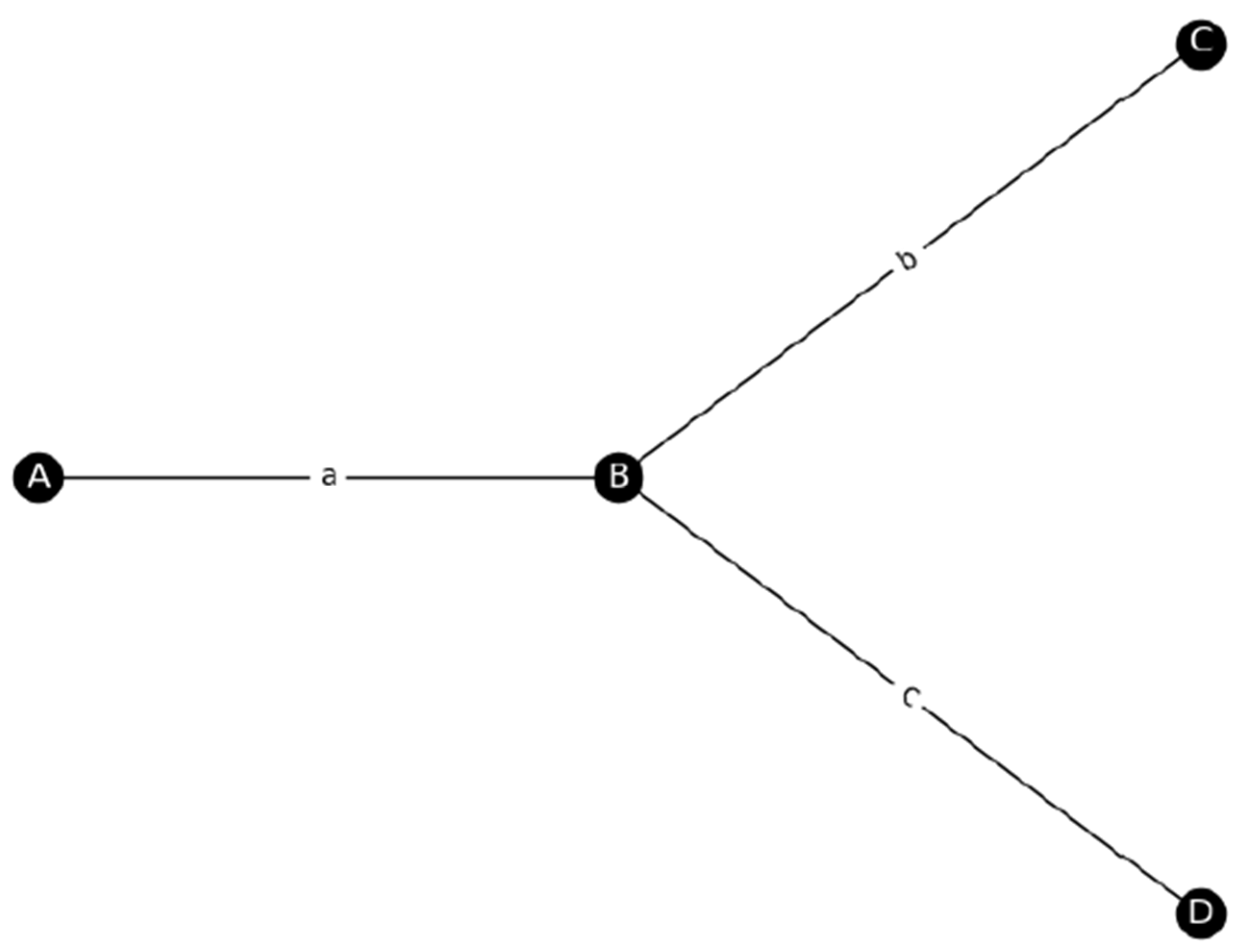
3.1. Simulations of Single-Looped Networks

Because of the complexity of the massflow calculation the used method was tested on five different testcases. Each testcase represents a different heating network with a specific issue regarding the network. While testcases 1 and 2 represent a single pipe and a network with two single branches, testcases 3 and 4 are of particular importance due to their interacting loops. All testcases, which are not explicitly presented here, can be viewed in the Appendix A. Testcase 3 presents a heating network with just one loop between nodes B, C and D and can be seen in Figure 3:

For analysis purposes and a fast computational time, the transient simulation calculated only 1 min of network behavior. In the first 30 s node A was the sole source of the network supplying the consumers with a constant temperature of 100 °C and delivering a constant massflow of 4 kg/s. Nodes E, D and F are the sole consumers in the first 30 s demanding 1 kg/s, 2 kg/s and 1 kg/s, respectively. After 30 s a second source was added, changing the node E from a consumer to a supplier. Additionally, the temperature in source A was reduced to 70 °C, while the temperature in source E was set to a constant temperature of 100 °C. At the same time, the massflow of node A was reduced from 4 kg/s to 2 kg/s and the massflow of the second source E was increased to meet the same massflow demands of the network (increased to 2 kg/s). Furthermore, nodes C, D and F were changed to consumer nodes, with a massflow demand of 1 kg/s, 1 kg/s and 2 kg/s. Figure 4 presents a short illustration of the transient behavior of the system.

The visualization of testcase 3 shows that in the first 30 s supplier A manages to fully supply all consumers. While it takes around 14 s for consumer E to fully heat up, at the same time a mixed temperature of 66 °C occurs at node D. At first this mixed temperature at node D is transported to node F. After around 16 s node D is also fully heated and transports the high temperature down to consumer F. Consumer F is the last consumer to fully heat up and needs around 20 s. After the first 30 s the second network behavior test starts with a fully heated network. After 38 s node B’s temperature decreases because of the temperature reduction in source A, while simultaneously node C’s temperature is kept constant due to the new source E. After 44 s a new mixed temperature at node D occurs around 87 °C, resulting from the temperatures of source E and A. Just as before, this new mixed temperature is then delivered to consumer F. Additionally, around 48 s a small temperature decrease in node C can be seen. Similar to node D, this temperature decreases results from the mixing of source A and E.

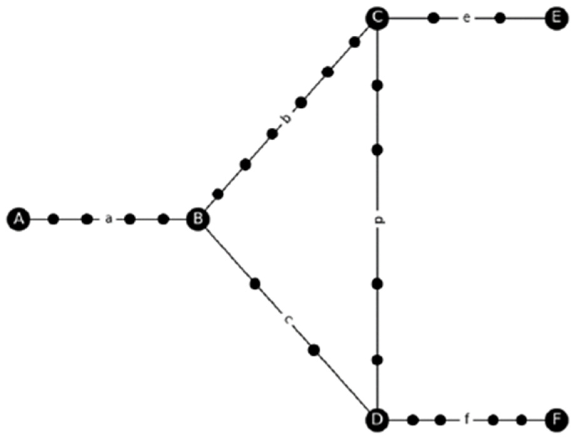
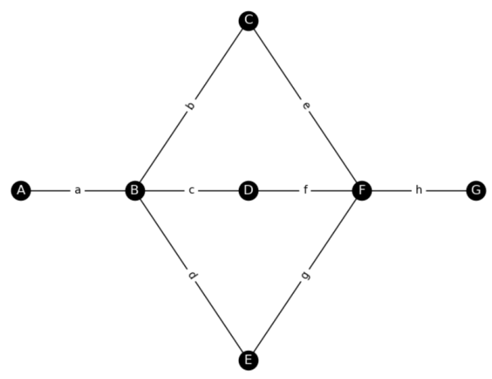
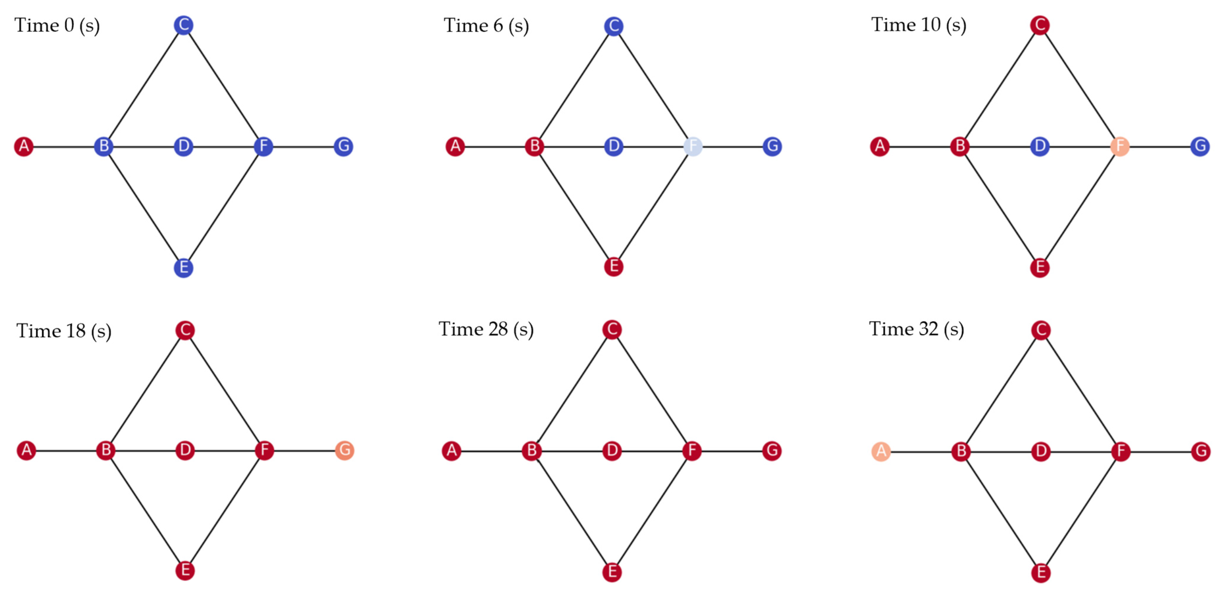
3.2. Simulations of Multiple-Looped Networks

Testcase 4 represents a heating network with three interacting loops. One loop between Node B, D, F and C. One loop between nodes B, D, F and E. And another loop between nodes B, C, F and E. The network of testcase 4 can be seen in Figure 5.

Similar to testcase 3, testcase 4 was simulated for 1 min. The first 30 s of the simulation node A is the only supplier of the network, while node G is the only consumer. Supplier A has a constant temperature of 100 °C and a massflow of 4 kg/s. After the first 30 s, supplier A’s temperature was reduced to 70 °C and its massflow to 1 kg/s. At the same time node D was changed to a second supplier with a massflow of 3 kg/s and a source temperature of 100 °C. In both cases, consumer G is the only consumer of the network with a constant massflow of 4 kg/s. Figure 6 presents the transient behavior of presented system.

Similar to testcase 3 testcase 4′s simulation presents, that in the first 30 s supplier A manages to fully supply every node. However, due to the multiple-loop network, multiple different mixing temperatures at node F can be seen throughout the first 30 s. The first mixed temperature caused by the temperature of the lowest network branch results in a mixing temperature of 43.49 °C. The second mixing temperature of 79.31 °C occurs around 10 s, when the temperature of the upper network branch arrives at node F. Finally, the last mixing temperature of node F can be seen around 18 s, when the temperature of the middle branch fully arrives at node F. Throughout the whole simulation it is noticeable that each mixing temperature arrives at the consumer G. After the first 30 s it is noticeable that supplier A’s temperature has been reduced. Meanwhile node D has been changed to a second supplier. Although there are now two suppliers in the system, a temperature reduction in all other nodes can be seen after 60 s. Consumer G’s temperature was reduced from 99 °C in the first 30 s to 92.4 °C after 60 s. The reason for this temperature drop is the mixing temperature at node B and the backflow of supplier D. Because supplier A’s massflow has been reduced and supplier D’s massflow has been increased, a backflow of source D to node B is occurring. This new backflow results in a new mixed temperature at node B, which is then transported to node C, E and finally again mixed at node F. This final mixed temperature at node F with a temperature of 92.49 °C is then transported to consumer G, resulting in a temperature reduction at the consumer despite two independent sources.

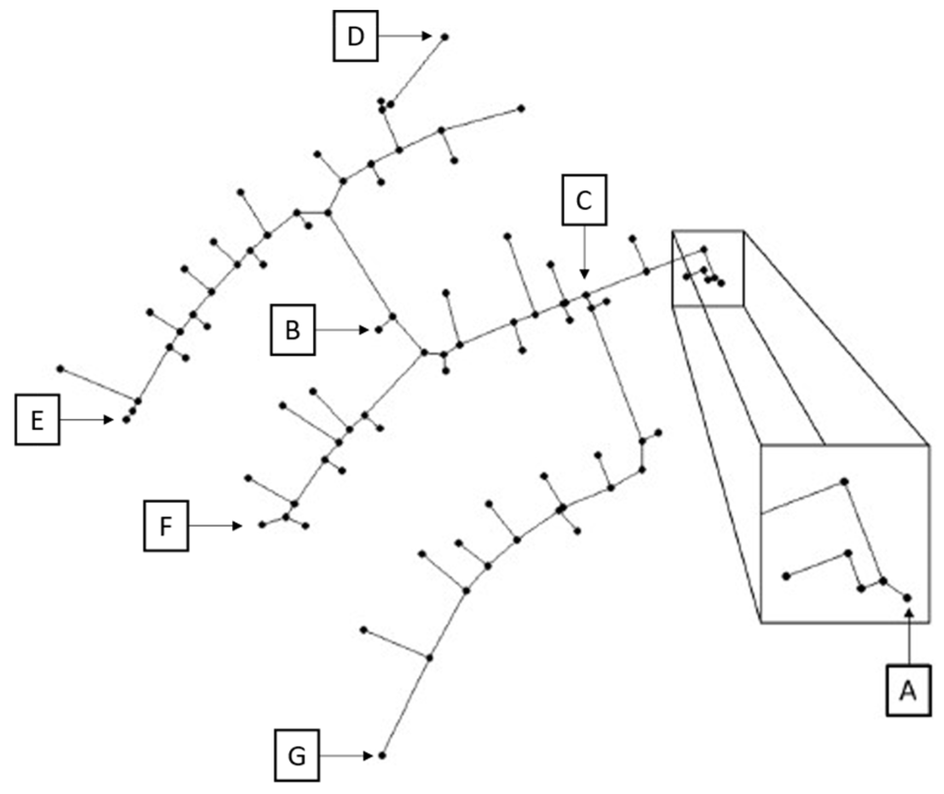
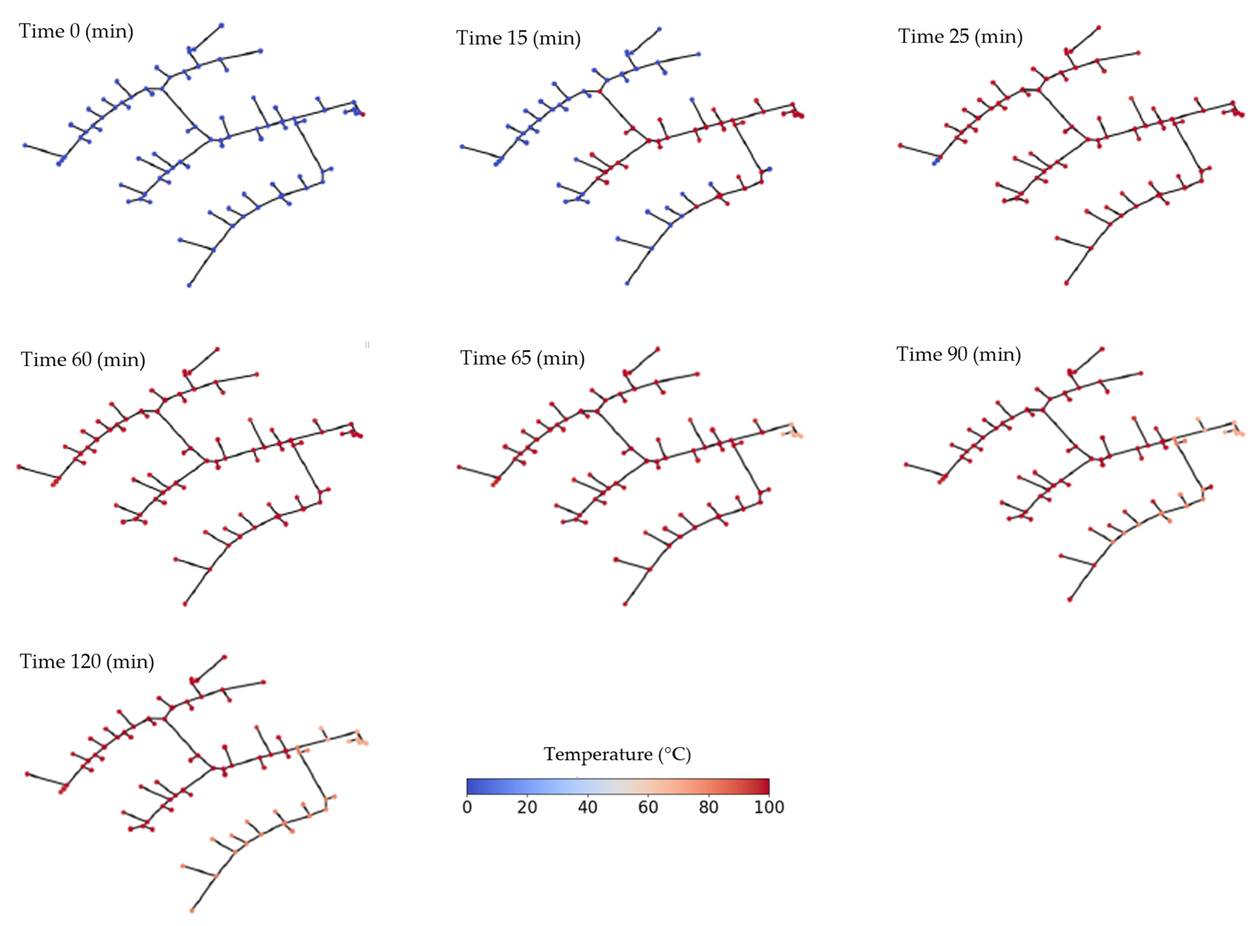
3.3. Simulations of a Non-Looped Networks

Testcase 5 was the last heating network to be tested. It is the biggest testcase and represents a real heating district. In comparison to the other presented testcases it defines itself as a non-looped network, where 1 h in total was simulated. Figure 7 presents the non-looped heating network.

Similar to the other testcases, two different behaviors were simulated. In the first 30 min the heating district was supplied with only one supplier in node A. After the first 30 min a second supplier B was added. Supplier A delivered a constant temperature of 100 °C in the first 30 min. After the 30 min and while supplier B was active, suppliers A temperature was reduced from 100 °C to 70 °C. At the same time the massflow of supplier A was reduced by a factor of 4.7 and the massflow of supplier B was increased to meet the same massflow demand of the heating network. Supplier B also supplied the network with a constant temperature of 100 °C. For the later discussion, temperatures and massflows of nodes C, D, E, F and G were noted. These nodes are the last nodes of each branch of the presented heating network and thus were chosen for the later comparison. Figure 8 presents a visualization of the network behavior.

Significant in Figure 8 is how the temperatures in the simulated network behave. It is noticeable that in the first 30 min supplier A managed to fully supply all nodes with a high temperature. Node G takes the longest to heat up. Additionally, it is also noticeable, how the activation of the second supplier changes the network behavior. While the second supplier is active, the heating network can be divided into two regions. The upper region of the heating network, which is only supplied by supplier B and the lower branch of the heating network, which is supplied by a mixed temperature of supplier A and B. This mixed temperature occurs at node C and is transported down the lower branch of the heating network.

4. Discussion

For the validation of the simulations method, the results of the testcases have been compared with results from the software Epanet and theoretical results via a manual calculation. In this context, for the validation of the hydraulic model and the calculated massflows, the software Epanet is used. For the validation of the transient temperatures a manual calculation of the networks’ temperature steady state is calculated and compared to the simulations result.

Table 1. Testcase 3, Comparison massflow results between simulation and Epanet.

	0–30 s		30–60 s
Pipe	Massflow Simulation (kg/s)	Massflow Epanet (kg/s)	Massflow Simulation (kg/s)	Massflow Epanet (kg/s)
a	4	4	4	4
b	1	1	3	3
c	3	3	1	1

,

Table 2. Testcase 4, Comparison massflow results between simulation and Epanet.

	0–30 s		30–60 s
Pipe	Massflow Simulation (kg/s)	Massflow Epanet (kg/s)	Massflow Simulation (kg/s)	Massflow Epanet (kg/s)
a	4	4	2	2
b	2.01	1.95	0.77	0.77
c	1	1	−2	−2
d	1.99	2.05	1.23	1.23
e	1	1	2	2
f	1.01	0.95	1.77	1.77

and

Table 3. Testcase 5, Comparison massflow results between simulation and Epanet.

	Hour 1		Hour 2
Node	Massflow Simulation (kg/s)	Massflow Epanet (kg/s)	Massflow Simulation (kg/s)	Massflow Epanet (kg/s)
A	−2.53	−2.53	−0.53	−0.53
B	0.03	0.03	−1.97	−1.97
C	0.73	0.73	0.73	0.73
D	0.20	0.20	0.20	0.20
E	0.02	0.02	0.02	0.02
F	0.24	0.24	0.24	0.24
G	0.20	0.20	0.20	0.20

compare the massflow calculation of the presented testcases with the massflow calculation of Epanet:

Throughout Table 1, Table 2 and Table 3 it is visible that the hydraulic model calculates in nearly every case the same massflow distribution as the software Epanet. The largest massflow deviation of 0.06 kg/s can be seen in testcase 4 in the first 30 s. However, it is also noticeable, that all changes in massflows as well as potential backflows were correctly approximated by the hydraulic model.

As mentioned before, in the case of the temperature comparison the simulated temperatures were compared to a manual calculation of the steady-state temperatures of each network. The reason why this comparison has been made is because unfortunately no real temperature measurements of the presented networks exist. By using the theoretical steady-state temperatures not only can the temperature values of the transient simulations be compared but moreover the time validated at which the transient simulation should occur at which node. This comparison can be performed because every transient simulation converges until a steady state is reached. By comparing the theoretical steady state with the transient simulation, conclusions about the transient simulation can be drawn. In general, deviations between the steady-state solution and the transient solution indicate that the transient simulation itself calculates incorrectly.

Table 4. Testcase 3, comparison between temperatures simulation (left) and theoretical temperatures (right).

	Simulation							Theoretical Values
	Time (s)	A (°C)	B (°C)	C (°C)	D (°C)	F (°C)	E (°C)	Time(s)	A (°C)	B (°C)	C (°C)	D (°C)	F (°C)	E (°C)
0–30 s	0	100	0	0	0	0	0	0	100	0	0	0	0	0
	2	100	0	0	0	0	0	-	100	0	0	0	0	0
	4	100	99.67	0	0	0	0	3.76	100	99.99	0	0	0	0
	6	100	99.99	0	0	0	0	-	100	99.99	0	0	0	0
	8	100	99.99	99.99	66.26	0	0	7.5/7.54	100	99.99	99.99	66.31	0	0
	10	100	99.99	99.99	66.31	0	0	-	100	99.99	99.99	-	0	0
	12	100	99.99	99.99	66.31	66.30	99.99	11.30/11.26	100	99.99	99.99	-	66.30	99.99
	14	100	99.99	99.99	66.31	66.30	99.99	-	100	99.99	99.99	-	-	99.99
	16	100	99.99	99.99	99.99	66.30	99.99	14.93	100	99.99	99.99	99.996	-	99.99
	18	100	99.99	99.99	99.99	66.30	99.99	-	100	99.99	99.99	99.996	-	99.99
	20	100	99.99	99.99	99.99	99.99	99.99	18.69	100	99.99	99.99	99.996	99.99	99.99
	30	100	99.99	99.99	99.99	99.99	99.99	-	100	99.99	99.99	99.996	99.99	99.99
30–60 s	32	70	99.99	99.99	99.99	99.99	100	32	70	-	-	-	-	100
	38	70	69.99	99.99	99.99	99.99	100	37.52	70	69.99	-	-	-	100
	40	70	69.99	99.99	99.99	99.99	100	-	70	69.99	-	-	-	100
	44	70	69.99	99.99	87.90	99.99	100	43.63	70	69.99	-	87.70	-	100
	46	70	69.99	91.66	87.70	87.81	100	-	70	69.99	-	-	-	100
	48	70	69.99	91.66	87.70	87.70	100	47.27	70	69.99	91.66	-	-	100
	50	70	69.99	91.66	87.70	87.70	100	-	70	69.99	91.66	-	-	100
	52	70	69.99	91.66	82.81	87.70	100	51.52	70	69.99	91.66	82.78	-	100
	54	70	69.99	91.66	82.78	82.80	100	53.40	70	69.99	91.66	82.78	82.78	100
	56	70	69.99	91.66	82.78	82.78	100	-	70	69.99	91.66	82.78	82.78	100
	60	70	69.99	91.66	82.78	82.78	100	-	70	69.99	91.66	82.78	82.78	100

,

Table 5. Testcase 4, comparison between temperatures simulation (left) and theoretical temperatures (right).

	Simulation								Theoretical Values
	Time (min)	A (°C)	B (°C)	C (°C)	D (°C)	E (°C)	F (°C)	G (°C)	Time (min)	A (°C)	B (°C)	C (°C)	D (°C)	E (°C)	F (°C)	G (°C)
0–30 s	0	100	0	0	0	0	0	0	0	100	0	0	0	0	0	0
	2	100	57.46	0	0	0	0	0	2.1	100	99.99	0	0	0	0	0
	4	100	99.99	0	0	0	0	0	-	100	99.99	0	0	0	0	0
	6	100	99.99	0	0	99.99	43.5	0	4.6/5.1	100	99.99	0	0	99.99	43.5	0
	8	100	99.99	99.99	0	99.99	43.5	0	6.7	100	99.99	99.99	0	99.99	-	0
	10	100	99.99	99.99	0	99.99	69.8	0	10	100	99.99	99.99	0	99.99	79.31	0
	12	100	99.99	99.99	0	99.99	79.31	0	-	100	99.99	99.99	0	99.99	-	0
	14	100	99.99	99.99	99.76	99.99	79.31	43.5	13.7/12.3	100	99.99	99.99	99.99	99.99	-	43.5
	16	100	99.99	99.99	99.99	99.99	79.31	43.5	-	100	99.99	99.99	99.99	99.99	-	-
	18	100	99.99	99.99	99.99	99.99	99.99	79.31	17.3/17.2	100	99.99	99.99	99.99	99.99	99.99	79.31
	20	100	99.99	99.99	99.99	99.99	99.99	79.31	-	100	99.99	99.99	99.99	99.99	99.99	99.99
	28	100	99.99	99.99	99.99	99.99	99.99	99.99	-	100	99.99	99.99	99.99	99.99	99.99	99.99
30–60 s	30	70	99.99	99.99	100	99.99	99.99	99.99	30	70	-	-	100	-	-	-
	32	70	99.99	99.99	100	99.99	99.99	99.99	-	70	-	-	100	-	-	-
	38	70	99.99	99.99	100	99.99	99.99	99.99	-	70	-	-	100	-	-	-
	40	70	90.36	99.99	100	99.99	99.99	99.99	38.2	70	90.36	-	100	-	-	-
	42	70	90.36	99.99	100	90.36	95.9	99.99	40.8	70	90.36	-	100	90.36	-	-
	44	70	90.36	90.36	100	90.36	95.9	99.99	43	70	90.36	90.36	100	90.36	-	-
	46	70	90.36	90.36	100	90.36	95.9	99.99	-	70	90.36	90.36	100	90.36	-	-
	48	70	90.36	90.36	100	90.36	92.5	99.99	46.3	70	90.36	90.36	100	90.36	92.5	-
	50	70	90.36	90.36	100	90.36	92.5	95.87	-	70	90.36	90.36	100	90.36	92.5	-
	52	70	90.36	90.36	100	90.36	92.5	95.87	-	70	90.36	90.36	100	90.36	92.5	-
	54	70	90.36	90.36	100	90.36	92.5	92.56	53.5	70	90.36	90.36	100	90.36	92.5	92.49
	60	70	90.36	90.36	100	90.36	92.5	92.49	-	70	90.36	90.36	100	90.36	92.5	92.49

and

Table 6. Testcase 5, comparison between temperatures simulation (left) and theoretical temperatures (right).

	Simulation								Theoretical Values
	Time (min)	A (°C)	B (°C)	C (°C)	D (°C)	E (°C)	F (°C)	G (°C)	Time (min)	A (°C)	B (°C)	C (°C)	D (°C)	E (°C)	F (°C)	G (°C)
Hour 1	0	100	0	0	0	0	0	0	0	100	0	0	0	0	0	0
	4	100	0	99.85	0	0	0	0	3.16	100	0	99.85	0	0	0	0
	-	100	0	99.85	0	0	0	0	-	100	0	99.85	0	0	0	0
	13	100	0.46	99.85	0	0	0	0	13.11	100	98.50	99.85	0	0	0	0
	14	100	98.50	99.85	0	0	0	0	-	100	98.50	99.85	0	0	0	0
	-	100	98.50	99.85	0	0	0	0	-	100	98.50	99.85	0	0	0	0
	20	100	98.50	99.85	0	0	98.27	0	19.77	100	98.50	99.85	0	0	98.27	0
	21	100	98.50	99.85	98.22	0	98.27	97.51	20.44/20.29	100	98.50	99.85	98.22	0	98.27	97.51
	-	100	98.50	99.85	98.22	0	98.27	97.51	-	100	98.50	99.85	98.22	0	98.27	97.51
	28	100	98.50	99.85	98.22	94.04	98.27	97.51	27.85	100	98.50	99.85	98.22	95.47	98.27	97.51
	29	100	98.50	99.85	98.22	95.47	98.27	97.51	-	100	98.50	99.85	98.22	95.47	98.27	97.51
Hour 2	61	70	100	99.85	98.22	95.47	98.27	97.51	61	70	100	99.85	98.22	95.47	98.27	97.51
	70	70	100	99.40	98.71	95.47	98.27	97.51	69.91	70	100	-	98.70	-	-	-
	71	70	100	99.36	98.71	95.47	98.26	97.51	-	70	100	-	98.70	-	-	-
	-	70	100	-	98.71	-	-	-	-	70	100	-	98.70	-	-	-
	73	70	100	99.27	98.71	95.47	98.54	97.51	72.94	70	100	-	98.70	-	98.55	-
	74	70	100	99.22	98.71	95.47	98.56	97.51	-	70	100	-	98.70	-	98.55	-
	-	70	100	-	98.71	-	98.56	-	-	70	100	-	98.70	-	98.55	-
	78	70	100	80.76	98.71	95.94	98.56	97.47	77.32	70	100	-	98.70	95.94	98.55	-
	-	70	100	-	98.71	95.94	98.56	-	-	70	100	-	98.70	95.94	98.55	-
	87	70	100	80.72	98.71	95.94	98.56	97.08	86.64	70	100	80.72	98.70	95.94	98.55	-
	-	70	100	80.72	98.71	95.94	98.56	-	-	70	100	80.72	98.70	95.94	98.55	-
	104	70	100	80.72	98.71	95.94	98.56	78.83	103.76	70	100	80.72	98.70	95.94	98.55	78.83

present the temperature comparison of each testcase.

Table 4 presents the temperature comparison of testcase 3. On the left side of the table are the results of the transient simulation, while on the right side of the table are the above-mentioned theoretical steady-state results. The upper half of the table covers the first 30 s of the simulation, while the lower half presents the later 30 s of the testcase. Noticeable is that both the absolute temperature values as well as the arrival times of the simulation match the theoretical steady-state values of the manual calculation. Additionally, the above-mentioned mixing temperature at node D is also well approximated in the simulations. The first mixing occurs around 8 s with a temperature of 66.31 °C, while the second mixing occurs around 15 s with a final temperature of 99.99 °C. Both mixed temperatures are then transported to node F. After the first 30 s the two new mixing temperatures at node D (at 44 s and at 52 s) are also well approximated by the simulation. Even the above-mentioned slight temperature reduction at node C matches the theoretical results. The largest temperature deviation of this testcase is 0.21 °C. In the following table testcase 4 temperature comparison is presented.

In the same manner as Table 4 and Table 5 presents the temperature comparison of the simulation and the theoretical steady-state values. The table shows that the simulation results approximate the theoretical results to a sufficient degree. Significant are the three mixing temperatures at node F, which each are, respectively, transported to node G. Every mixed temperature matches in the value and the time the theoretical results. After the first 30 s the temperature reduction in every node despite two heating sources can also be seen. The largest temperature deviation of testcase 4 is 0.001 °C. Table 6 presents the temperature comparison of the last testcase.

Table 6 presents that the simulated results closely approximate the theoretical results of a non-looped network. The calculated temperature values as well as the arriving times of the simulated temperatures match the theoretical steady-state calculation. Additionally, node E takes the longest to heat up in the first hour. The second hour starts with the already heated network and the source switch of node B. Through this switch, a mixing occurs around 78 min at node C, which is then transported down the lower network branch and arrives at node G. Therefore, node G takes the longest to reach its steady state in the second hour. Significant is that although the theoretical values indicate that a temperature of 80 °C should be mixed at node C around 86 min, the transient simulate shows that this mixed temperature of 80 °C already arrives at around 78 min. The reason why the transient simulation presents a much earlier arriving time of the fluid is because the second hour starts with an already heated network. This new temperature distribution is then carried by the new massflow and results in an earlier mixing temperature than the theoretical results. This particular result can lead to the suspicion that the temperature and massflow of supplier A could be further reduced, since the occurring mixing happens quite timely with the high temperature of the network after 1 h. It is worth noting that such time- and network-dependent results can only be obtained through transient simulation and can lead to new and more optimized heating districts. Although the presented results indicate only a small difference to the steady-state solution, it is quite apparent how such transient results could become more significant in larger and more complex networks.

In summary it can be said that all the presented testcases here are well approximated by the transient simulation. Both the massflow calculations of the hydraulic model as well as the numerical solution of the thermodynamic and comprehensive model match the results from Epanet or the steady-state solution. Additionally, it needs to be mentioned that especially the last testcase indicates why a transient simulation can be of interest for the calculation of a heating districts.

However, it is important to note that while the temperatures are calculated using a transient differential equation the calculated massflows are assumed to be constant. This assumption introduces an error into the solution, as the massflow change is assumed to be abrupt. In reality the massflows adjust gradually through the pressure difference in each pipe and the networks layout. Calculating the correct massflow change in a heating network is, however, very computational demanding and is only used in very small networks and via a suitable working station. As mentioned in the literature comparison, some sources also use a constant massflow assumption as a valid approximation due to the difficulties of their correct calculation [5,7,11,18,19]. The presented simulation method is in theory capable of simulating the time-dependent temperature changes based on the transient massflow changes if a suitable transient hydraulic model is implemented via, for example, a manual table or mathematical approximation. Additionally due to the simulation method being a simplified method for the correct heat wave propagation, the actual error of this simplification needs to be further studied. Effects like the heating and cooling down of the network’s pipes can lead to different temperature dynamics and thus realistic arrival times of the heat wave. However, the simulation method presents a first easy step for the simulation of transient district heating behavior and a course approximation of how a heating network could behave based on the presented suppliers, consumers and network layout.

5. Conclusions

This work presents a simple transient simulation method based on state-space modeling of heating networks. The usage and the results of transient heating district can lead to a better understanding of the network’s behavior and thus to a more optimized operation of heating districts. Especially with the current trends of more decentralized suppliers and more flexible consumers, the need for transient simulation for heating district is gaining more importance. The presented algorithm focuses on an easy to implement simulation method for a transient simulation of looped or non-looped networks. Additionally, time-dependent changes and time-dependent switches of consumers to suppliers can be applied, which lead to different network behaviors as shown in the testcases. The simulation method presents a good numerical accuracy of temperature and arrival times, when compared to the steady-state solution of each network. Furthermore, the simulation method shows a sufficient approximation of the massflows distribution in single looped and multiple-loop networks.

Although the calculation of the simulation method presents an overall good approximation, it is important to mention the computational effort each simulation requires. Due to the numerical background of the simulation method, larger networks need more calculation nodes for sufficient approximation. This increase in calculation nodes can lead to larger matrices and thus to a higher computational workload and time. In conclusion, this means that the algorithm should only be used for smaller networks, while it can be adapted for larger networks by a more optimized coding involving, for example, sparsematrix or quick-search algorithms.

References

1. Schojda, D.; Scheipers, J.; Roes, J.; Hoster, H. Modelling and Simulation of Transient District Heating Networks Based on a Control Theory Approach. In Proceedings of the 19th Conference on Sustainable Development of Energy Water and Environment Systems (SDEWES 2024), Rome, Italy, 9–13 September 2024. [Google Scholar]
2. Jie, P.; Tian, Z.; Yuan, S.; Zhu, N. Modeling the dynamic characteristics of a district heating network. Energy 2012, 39, 126–134. [Google Scholar] [CrossRef]
3. Stevanovic, V.D.; Zivkovic, B.; Prica, S.; Maslovaric, B.; Karamarkovic, V.; Trkulja, V. Prediction of thermal transients in district heating systems. Energy Convers. Manag. 2009, 50, 2167–2173. [Google Scholar] [CrossRef]
4. Gabrielaitiene, I.; Bøhm, B.; Sunden, B. Modelling temperature dynamics of a district heating system in Naestved, Denmark—A case study. Energy Convers. Manag. 2007, 48, 78–86. [Google Scholar] [CrossRef]
5. Del Hoyo Arce, I.; López, S.H.; Perez, S.L.; Rämä, M.; Klobut, K.; Febres, J.A. Models for fast modelling of district heating and cooling networks. Renew. Sustain. Energy Rev. 2018, 82, 1863–1873. [Google Scholar] [CrossRef]
6. Oppelt, T.; Urbaneck, T.; Gross, U.; Platzer, B. Dynamic thermo-hydraulic model of district cooling networks. Appl. Therm. Eng. 2016, 102, 336–345. [Google Scholar] [CrossRef]
7. Licklederer, T.; Hamacher, T.; Kramer, M.; Perić, V.S. Thermohydraulic model of Smart Thermal Grids with bidirectional power flow between prosumers. Energy 2021, 230, 120825. [Google Scholar] [CrossRef]
8. van der Heijde, B.; Fuchs, M.; Ribas Tugores, C.; Schweiger, G.; Sartor, K.; Basciotti, D.; Helsen, L. Dynamic equation-based thermo-hydraulic pipe model for district heating and cooling systems. Energy Convers. Manag. 2017, 151, 158–169. [Google Scholar] [CrossRef]
9. Guelpa, E. Impact of network modelling in the analysis of district heating systems. Energy 2020, 213, 118393. [Google Scholar] [CrossRef]
10. Menapace, A.; Avesani, D. Global Gradient Algorithm Extension to Distributed Pressure Driven Pipe Demand Model. Water Resour Manag. 2019, 33, 1717–1736. [Google Scholar] [CrossRef]
11. Vesterlund, M.; Toffolo, A.; Dahl, J. Simulation and analysis of a meshed district heating network. Energy Convers. Manag. 2016, 122, 63–73. [Google Scholar] [CrossRef]
12. Becker, G.; Klemm, C.; Vennemann, P. Open Source District Heating Modeling Tools—A Comparative Study. Energies 2022, 15, 8277. [Google Scholar] [CrossRef]
13. Sartor, K.; Thomas, D.; Dewallef, P. A comparative study for simulating heat transport in large district heating networks. Int. J. Heat Technol. 2018, 36, 301–308. [Google Scholar] [CrossRef]
14. Blommaert, M.; Wack, Y.; Baelmans, M. An adjoint optimization approach for the topological design of large-scale district heating networks based on nonlinear models. Appl. Energy 2020, 280, 116025. [Google Scholar] [CrossRef]
15. Larsen, H.V.; Pálsson, H.; Bøhm, B.; Ravn, H.F. Aggregated dynamic simulation model of district heating networks. Energy Convers. Manag. 2002, 43, 995–1019. [Google Scholar] [CrossRef]
16. Zheng, W.; Hou, Y.; Li, Z. A Dynamic Equivalent Model for District Heating Networks: Formulation, Existence and Application in Distributed Electricity-Heat Operation. IEEE Trans. Smart Grid 2021, 12, 2685–2695. [Google Scholar] [CrossRef]
17. Ancona, M.A.; Melino, F.; Peretto, A. An Optimization Procedure for District Heating Networks. Energy Procedia 2014, 61, 278–281. [Google Scholar] [CrossRef]
18. Çengel, Y.A. Heat Transfer: A Practical Approach, 2nd ed.; McGraw-Hill Series in Mechanical Engineering; McGraw-Hill: Boston, MA, USA, 2003. [Google Scholar]
19. Zhang, S.; Pan, G.; Li, B.; Gu, W.; Fu, J.; Sun, Y. Multi-Timescale Security Evaluation and Regulation of Integrated Electricity and Heating System. IEEE Trans. Smart Grid 2024, 1. [Google Scholar] [CrossRef]
20. Jiang, M.; Speetjens, M.; Rindt, C.; Smeulders, D. A data-based reduced-order model for dynamic simulation and control of district-heating networks. Appl. Energy 2023, 340, 121038. [Google Scholar] [CrossRef]
21. Bastida, H.; Ugalde-Loo, C.E.; Abeysekera, M.; Qadrdan, M.; Wu, J. Thermal Dynamic Modelling and Temperature Controller Design for a House. Energy Procedia 2019, 158, 2800–2805. [Google Scholar] [CrossRef]
22. Chua, L.O.; Lin, P.-M. Computer-Aided Analysis of Electronic Circuits: Algorithms and Computational Techniques; Prentice-Hall Series in Electrical and Computer Engineering; Prentice-Hall: Englewood Cliffs, NJ, USA, 1975. [Google Scholar]
23. Liu, X.; Jenkins, N.; Wu, J.; Bagdanavicius, A. Combined Analysis of Electricity and Heat Networks. Energy Procedia 2014, 61, 155–159. [Google Scholar] [CrossRef]
24. Liu, X. Combined Analysis of Electricity and Heat Networks. Ph.D. Thesis, Cardiff University, Cardiff, Wales, 2013. [Google Scholar]
Figure 1. Left side example of a simplistic heating network (no interacting loop), right side example of a complex heating network (one interacting loop).
Energies 18 00658 g001
Figure 2. Example of a main node and sub-node distribution.
Energies 18 00658 g002
Figure 3. Testcase 3, network with just one interacting loop.
Energies 18 00658 g003
Figure 4. Visualization testcase 3. Transient simulation of one looped network.
Energies 18 00658 g004
Figure 5. Testcase 4, network with multiple interacting loops.
Energies 18 00658 g005
Figure 6. Visualization testcase 4. Transient simulation of multiple-loop network.
Energies 18 00658 g006aEnergies 18 00658 g006b
Figure 7. Testcase 5, non-looped real heating network.
Energies 18 00658 g007
Figure 8. Visualization testcase 5. Transient simulation of multiple-loop network.
Energies 18 00658 g008