Deep-Learning Techniques Applied for State-Variables Estimation of Two-Mass System

Abstract

The article is focused on the application of neural models for state-variables estimation. The estimators are applied in the control structure (with the state speed controller) of the electric drive with an elastic shaft. The extended amount of feedback is an additional argument for the estimation of the signal. The calculations are performed for three deep neural structures based on the Convolutional Neural Network (CNN) and the long short-term memory (LSTM). The design stages and the overall concept in this case are completely different than with the applications of classical observers (e.g., the Luenberger, the Kalman filter) often used for similar objects. The direct identification of the mechanical part of the drive is not necessary. The parameters and the equations describing the plant are not used. Instead, the signals are used for training the neural networks. The results (performed for the nominal values of the two-mass system and presenting the robustness of the estimators) present the high precision of the signal estimation. The second part of the work deals with the hardware implementation of the neural estimators in the low-cost programmable device with the ARM core. The experimental transients confirm the features of the neural estimators noticed in the simulations.

1. Introduction

Electric drives are one of the most important components of automation systems noticed in the industry. The efficiency of the technological process depends on the precision and reliability of the elements of the drives. Therefore, the works performed in the research units focus mainly on the development and application of new machines, improvements of the power-electronics devices, diagnostics, and the implementation of new algorithms [1,2,3,4,5,6,7]. The most interesting solutions, which commonly do not require modification of the hardware structure of the system, are related to the control methods. Presently, they also include the techniques known from the theory of artificial intelligence—neural networks and fuzzy logic models [8,9,10]. Considering the abovementioned electric drive requirements, the mechanical part of the overall construction should be taken into account. Non-linearities (backlash, friction of the machine, etc.) and elasticity of the shaft between the main motor and the load can cause serious disturbance—oscillations of state variables [11,12]. Damping of the signals and precise control with high dynamics can be impossible using conventional control strategies. For this purpose, advanced speed controllers are applied for the drives. However, the point connecting the applied structures (even in the case of modified classical controllers) is the extended number of feedback signals from the object. The control signal based on additional information can force the plant to strictly follow the reference trajectory in a stable manner [13,14,15].

The need for state-variable estimation related to the extended number of signals used in control structures becomes an even more important issue [16]. The drive with implemented sensors is more susceptible to the occurring faults. It requires the use of additional algorithms to monitor the condition of the system. It leads to higher costs of construction. Moreover, the implementation of the encoders or elements measuring the current can be problematic on a real drive. Based on the abovementioned arguments, numerous algorithms for the estimation of state variables in electric drives are found in the literature [17,18,19,20]. Analyzing the papers published in the journals (or the proceedings of conferences) focused on electric drives, control theory, and algorithms based on artificial intelligence, three groups of solutions can be distinguished: algorithmic methods (e.g., the Luenberger observer, the Kalman filter, Model Reference Adaptive Systems, etc.) [21,22,23], modern solutions (neural networks and fuzzy logic) [24,25], and hybrid techniques (combination of both previously pointed models) [26,27].

The commonly used state variables calculation methods for two-mass systems are based on equations related to their mechanical coupling [28,29]. Moreover, the correction matrix (including coefficients defined with time constants) is used for the final variables (e.g., load speed, shaft torque) estimation. The implementation does not need complex calculations. However, the precision of the signal estimation strictly depends on the precision of the object identification. Therefore, improvements to the Luenberger observer have been proposed. Adaptation of the algorithm parameters using the gradient method [30] or fuzzy modifications [31] can improve the precision of operation under changes in object parameters. The next issue related to the analyzed observers is the dynamics defined by the user. Their high level can be forced with the gains of the algorithm. Fast work is achieved as the parameters increase. However, it can lead to the amplification of measurement noise. Therefore, the correct selection of the observer coefficients is crucial for real applications. The authors have proposed adapting the gain matrix with respect to speed estimation error [32]. If the value is significant, the gain values are increased to reduce the error. In the opposite state, decreasing the coefficient values does not cause amplification of the disturbance. The main concept is obtained using a fuzzy model.

The second solution, significant in the group of algorithms based on mathematical equations and the parameters of the plant, is the Kalman filter. Here, the calculations are realized in cyclically repeated stages. The state vector from the previous step is a part of state prediction. Then, the actual values of the state variables are achieved using the predicted vector. The extended form of object equations leads to a more robust and easier-to-implement algorithm [33]. The Kalman filter was successfully implemented for the state-variables estimation of the two-mass system. It should be noted that the robustness of the control structure can be further improved by extending the Kalman filter’s state vector with the time constants of the load machine and the stiffness. Then, an online update of the values can be used to recalculate the speed control gains [34,35]. The specific points of the Kalman filter equations are the covariance matrices. The values depend on the measurements and object noise. It is significant for precise state estimation. However, the mathematical formula is difficult to obtain. Thus, for optimization, a genetic algorithm is used. Moreover, for the adaptation of the matrices, a fuzzy model can be implemented [36].

Recently, a new strategy of the state observer applied for the electric drive with elastic connection is noticed. It is based on the known Luenberger structures. The algorithms operate in parallel as the first layer of the observer. Then, the output signals are connected, according to the proposed formula, for the calculation of the output signals. The concept is known as the Multi-layer observer [37,38]. The results appear promising. The estimation errors are smaller than those obtained using the standalone Luenberger observer.

Neural networks have been proposed in the middle of the previous century. The initial concepts, structures, and training algorithms have been developed. Presently, regarding the progress noticed in the engineering tools (hardware—programmable devices and computing workstations, software—user-friendly libraries and standalone applications, and as a part of machine learning, one of the main elements—data available even through the widespread availability of the Internet), significant expansion of implementations is observed. It is related to various technical fields—including electric drives [8,39,40].

A completely different group of methods applied for the calculation of signals in electric drives is based on algorithms based on the theory of artificial intelligence. It can contain fuzzy logic algorithms and neural networks. The mentioned models can be used as standalone estimators or hybrid combination with classical observers. The examples of modifications proposed for classical observers are analyzed above. This part of the review focuses on the neural estimators applied for the drive with an elastic clutch between the machines. The neural networks are a typical representation of the assumptions in the field of machine learning. In contrast to classical model design, in this case, the model is created from the data. Then, a separate set of samples is used for tests. During the training process, the internal coefficients, i.e., weights, are optimized for a precise global representation of the process or system. If an appropriate dataset, learning algorithm, and neural network structure are used, it is possible to recover the state variables of a two-mass system. These assumptions present a different process of estimator design, where the direct use of equations and object parameters is omitted. Typically, for a drive with an elastic shaft, the motor speed and the current are assumed to be measurable. The load speed and the shaft torque are calculated with neural networks [41]. If the mathematical model is not used during the design stages, assuming an accurate representation of the signal trends, robustness can be expected. However, the feature is difficult to obtain but can be improved using the following methods: structure optimization, regularization, proper selection of the training data, settings of the training algorithms (e.g., the number of epochs) [8,42,43,44]. The crucial point seems to be related to the optimization of the neural network topology [45,46]. It is also significant for hardware implementation. The programmable device should be capable of performing the implemented neural processing (the basic unit is simple, but the network structure can demand high computational power). Moreover, the specific calculations should be taken into account. The structure consists of sequentially connected layers. However, the nodes in the layer are placed in parallel. An additional aspect during hardware selection is also its cost. Considering the above assumptions, three main solutions regarding hardware implementations of neural networks in electric drives are noticed in articles: digital signal processor, field programmable gate arrays, and low-cost microcontrollers [47,48,49,50].

Presently, the subsequent generation of neural networks—Deep-Learning Neural Networks (DLNNs)—are commonly used [51,52]. It is an extension of previously developed shallow networks. The features of the mentioned models lead to numerous applications related to image processing and time-series data analysis. The article is focused on the original implementation of deep-learning algorithms for the calculation of signals from the mechanical part of the electric drive with the elastic shaft. The proposed solution could lead to a novel design method that assumes the optimization of estimator properties for more than one set of object parameters (including changes in time constant). It can be represented using the additional subset of data applied in the training process. Moreover, it also simplifies the design process for nonlinear systems. The initial applications of the DLNN in the processing of drive signals are presented in [53,54].

The manuscript presents original work that is an extension of the solutions presented in the articles so far. According to the trends noticed in the literature, the application of the considered deep-learning algorithms is a new path in the control theory and electric drives. The main contribution and novelty of the paper are defined by the following points.

• Presentation of the design, application, and tests of the state-variables estimators based on the Convolutional Neural Networks and the long short-term memory models. It should be noticed that the considered estimators contain typical operations from the CNN and the LSTM neural networks. However, the hybrid topology, which leads to promising results, is original.
• Implementation of the shaft torque and the motor speed deep neural estimators for the two-mass system. The simulation results present high precision of sample calculation and robustness against object parameter disturbances.
• The first part of the paper deals with theoretical considerations. The following step is dedicated to hardware implementation and experimental verification. For this purpose, the low-cost device was selected, and the algorithms were implemented using rapid prototyping tools.

The main contribution of the presented paper is the establishment of a deep neural network structure capable of torsional torque and motor speed estimation. The proposed neural network is also implementable in a low-cost programmable device and eligible for real-time operation. The article consists of six main parts. First, the analysis of the issues related to the electric drive with the elastic shaft is presented. The estimation task is highlighted and described. The next section presents the speed control structure applied for the two-mass system. Then, the proposed state estimators based on deep learning are shown (the topology and the design process). The following part is focused on the simulation tests. The subsequent description deals with the hardware implementation and the calculations performed for real data (measured on the laboratory drive). Next, the research based directly on samples from current and speed sensors is considered. The manuscript is finished with conclusions.

2. State Controller Applied for the Two-Mass System—A Mathematical Description

A two-mass system is a structure of two objects connected with a shaft characterized by finite stiffness. The torsional force and shaft flexibility cause many undesirable effects. Increased stress on the mechanical link may cause the elements to break. The decreased rigidity of the connection also makes the drive difficult to control. The twist of the shaft causes a difference between the angular speed of the motor and the load machine. As a result, the plant response is oscillatory and prone to overshooting. For such challenging plants, multivariable control with state feedback is often suggested. The state representation of the analyzed plant is given as [55]:

$$\dot{\mathit{x}}=\mathit{A}\mathit{x}+\mathit{B}u+\mathit{L}d$$

(1)

$$y=\mathit{C}\mathit{x}$$

(2)

where:

$$\mathit{x}=\left[\begin{array}{c}{\omega }_1\\ {\omega }_2\\ {\tau }_t\end{array}\right],\mathit{A}=\left[\begin{array}{ccc}0& 0& -{\displaystyle \frac{1}{T_1}}\\ 0& 0& {\displaystyle \frac{1}{T_2}}\\ {\displaystyle \frac{1}{T_t}}& -{\displaystyle \frac{1}{T_t}}& 0\end{array}\right],\mathit{B}=\left[\begin{array}{c}{\displaystyle \frac{1}{T_1}}\\ 0\\ 0\end{array}\right],$$

$$u={\tau }_e,d={\tau }_L,\mathit{L}=\left[\begin{array}{c}0\\ -{\displaystyle \frac{1}{T_2}}\\ 0\end{array}\right],\mathit{C}=\left[\begin{array}{ccc}0& 1& 0\end{array}\right],$$

${\omega }_1,{\omega }_2$—the angular speeds of the motor and load, ${\tau }_e,{\tau }_t,{\tau }_L$—the electromagnetic, torsional, and load torques, $T_1,T_2,T_t$—the mechanical time constants of the motor, load, and shaft. For the following considerations, it is assumed that the disturbance is ${\tau }_L=0$.

The goal of the synthesized control structure is to eliminate steady-state error and facilitate operation under external disturbances and parametric uncertainty. To achieve that, integral action must be incorporated into the feed-forward path of the structure. Therefore, the first step is to verify if there are no zeros positioned at $s=0$ that would cancel any manually inserted integrators. The transfer function $G\left(s\right)$ of the plant can be established with the following formula:

$$G\left(s\right)=\mathit{C}{(s\mathit{I}-\mathit{A})}^{-1}\mathit{B}$$

(3)

which, for the given example, yields

$$G\left(s\right)={\displaystyle \frac{1}{s\left(T_1{T}_2{T}_t{s}^2+T_1+T_2\right)}},$$

where s—the Laplace operator. Next, if a state controller is to be applied, the state controllability of the plant must be verified. The criterion is that the matrix $\mathsf{\Psi }$ must be of rank $n+1$ [56]:

$$rank\left(\mathsf{\Psi }\right)=rank\left(\left[\begin{array}{cc}\mathit{A}& \mathit{B}\\ -\mathit{C}& 0\end{array}\right]\right)=n+1,$$

(4)

where n is the number of variables in the state vector $\mathit{x}$. For the two-mass system:

$$rank\left({\mathsf{\Psi }}_{2mass}\right)=rank\left(\left[\begin{array}{cc}\mathit{A}& \mathit{B}\\ -\mathit{C}& 0\end{array}\right]\right)=4.$$

The proposed control law is given as:

$$u=-\mathit{K}\mathit{x}+k_I\zeta ,$$

(5)

where $\mathit{K},k_I$ are the controller gains, and $\zeta$ is a signal selected so that its derivative is equal to the control error e:

$$\dot{\zeta }=e={\omega }_{ref}-{\omega }_2={\omega }_{ref}-\mathit{C}\mathit{x}.$$

(6)

The approach to synthesizing a state feedback controller with integral action is to extend the state vector $\mathit{x}$ with the extra variable $\zeta$ [57]. The state equation of the control loop takes the following form:

$$\left[\begin{array}{c}\dot{\mathit{x}}\\ \dot{\zeta }\end{array}\right]=\left[\begin{array}{cc}\mathit{A}& \mathbf{0}\\ -\mathit{C}& 0\end{array}\right]\left[\begin{array}{c}\mathit{x}\\ \zeta \end{array}\right]+\left[\begin{array}{c}\mathit{B}\\ 0\end{array}\right]u+\left[\begin{array}{c}\mathbf{0}\\ 1\end{array}\right]{\omega }_{ref}$$

(7)

The designed system should be asymptotically stable. Assuming a step reference signal, for $t\to \infty$ the state variables $\mathit{x}$, $\zeta$ and the control signal u should settle at constant values with the output ${\omega }_2$ equal to ${\omega }_{ref}$. For any given time t, the difference between the current value of the signals and the final value in steady state can be defined:

$$\begin{array}{cc}\hfill \mathit{x}\left(t\right)-\mathit{x}(\infty )& ={\mathit{x}}_{ϵ}\left(t\right)\hfill \end{array}$$

(8)

$$\begin{array}{cc}\hfill \zeta \left(t\right)-\zeta (\infty )& ={\zeta }_{ϵ}\left(t\right)\hfill \end{array}$$

(9)

$$\begin{array}{cc}\hfill u\left(t\right)-u(\infty )& =u_{ϵ}\left(t\right)\hfill \end{array}$$

(10)

and also

$$u_{ϵ}=-\mathit{K}\mathit{x}+k_I{\zeta }_{ϵ}$$

(11)

Equations (8)–(10) can be inserted into the form of Equation (7) giving the following expression:

$$\left[\begin{array}{c}{\dot{\mathit{x}}}_{ϵ}\\ {\dot{\zeta }}_{ϵ}\end{array}\right]=\left[\begin{array}{cc}\mathit{A}& \mathbf{0}\\ -\mathit{C}& 0\end{array}\right]\left[\begin{array}{c}{\mathit{x}}_{ϵ}\\ {\zeta }_{ϵ}\end{array}\right]+\left[\begin{array}{c}\mathit{B}\\ 0\end{array}\right]u_{ϵ},$$

(12)

which, after substituting

$$ϵ=\left[\begin{array}{c}{\mathit{x}}_{ϵ}\\ {\zeta }_{ϵ}\end{array}\right],\tilde{\mathit{A}}=\left[\begin{array}{cc}\mathit{A}& \mathbf{0}\\ -\mathit{C}& 0\end{array}\right],\tilde{\mathit{B}}=\left[\begin{array}{c}\mathit{B}\\ 0\end{array}\right],$$

can be expressed as:

$$\dot{ϵ}=\tilde{\mathit{A}}ϵ+\tilde{\mathit{B}}{u}_{ϵ}.$$

(13)

Substituting the gain matrix $\mathit{K}$ to adhere to the new notation of the control signal $u_{ϵ}$:

$$\tilde{\mathit{K}}=\left[\begin{array}{cc}\mathit{K}& -k_I\end{array}\right],$$

(14)

Equation (11) now takes the following form:

$$u_{ϵ}=-\tilde{\mathit{K}}ϵ.$$

(15)

After inserting (15) into (13), the final description of the control structure is achieved:

$$\dot{ϵ}=(\tilde{\mathit{A}}-\tilde{\mathit{B}}\tilde{\mathit{K}})ϵ.$$

(16)

To find the gain matrix $\tilde{\mathit{K}}$, Ackermann’s formula [58] is utilized. The algorithm selects the gain values to place the eigenvalues of the control system’s state matrix at the desired poles. The reference polynomial $\vartheta \left(s\right)$ is selected as:

$$\vartheta \left(s\right)={(s^2+2\xi {\omega }_r+{\omega }_r^2)}^2=s^4+{\alpha }_1{s}^3+{\alpha }_2{s}^2+{\alpha }_{3}s+{\alpha }_4,$$

(17)

where $\xi$—the desired damping coefficient, ${\omega }_r$—the desired resonant frequency of the system, ${\alpha }_{1:4}$—the resulting reference polynomial coefficients. According to the Cayley-Hamilton theorem [59], the matrix $\tilde{\mathit{A}}-\tilde{\mathit{B}}\tilde{\mathit{K}}$ satisfies its own characteristic equation $\vartheta$:

$$\vartheta (\tilde{\mathit{A}}-\tilde{\mathit{B}}\tilde{\mathit{K}})=0$$

(18)

The following expression can now be defined:

$$\vartheta \left(\tilde{\mathit{A}}\right)={\tilde{\mathit{A}}}^4+{\alpha }_1{\tilde{\mathit{A}}}^3+{\alpha }_2{\tilde{\mathit{A}}}^2+{\alpha }_3\tilde{\mathit{A}}+{\alpha }_4\mathit{I}\ne 0.$$

(19)

Since the system has already been proven to be state-controllable, the inverse of the controllability matrix $\Gamma$ exists:

$$det(\Gamma )=det\left(\left[\begin{array}{cccc}\tilde{\mathit{B}}& \tilde{\mathit{A}}\tilde{\mathit{B}}& {\tilde{\mathit{A}}}^2\tilde{\mathit{B}}& {\tilde{\mathit{A}}}^3\tilde{\mathit{B}}\end{array}\right]\right)\ne 0.$$

(20)

The gains can be calculated using the following expression:

$$\tilde{\mathit{K}}=\left[\begin{array}{cccc}0& 0& 0& 1\end{array}\right]{\Gamma }^{-1}\vartheta \left(\tilde{\mathit{A}}\right).$$

(21)

After establishing the gain matrix $\tilde{\mathit{K}}$, Equations (5) and (7) can be combined to evaluate the proposed control structure:

$$\left[\begin{array}{c}\dot{\mathit{x}}\\ \dot{\zeta }\end{array}\right]=\left[\begin{array}{cc}\mathit{A}-\mathit{B}\mathit{K}& \mathit{B}{k}_I\\ -\mathit{C}& 0\end{array}\right]\left[\begin{array}{c}\mathit{x}\\ \zeta \end{array}\right]+\left[\begin{array}{c}\mathbf{0}\\ 1\end{array}\right]{\omega }_{ref}.$$

(22)

The graphical representation of the control structure is shown in Figure 1. The presented strategy is a cascade structure with an internal torque control loop. This loop consists of four elements: the electromagnetic part of the motor, a motor driver, a current controller, and a current sensor. It can be represented with the following transfer function:

$$G_e\left(s\right)={\displaystyle \frac{1}{T_{e}s+1}},$$

(23)

where $T_e$ is the time constant of the motor driver. With current advances in power electronics, the resulting torque generation delay can be considered negligible. Therefore, for the sake of simplification of the controller synthesis presented above, the torque control loop is assumed to be $G_e\left(s\right)=1.$

The presented structure requires three state–space variables to operate. The angular speed of the motor and the load can usually be easily obtained with the use of encoders, but the torsional torque measurement can be problematic. Therefore, the most efficient solution would be to establish a numerical tool for torque estimation. In this article, a deep neural network approach is proposed to solve this issue.

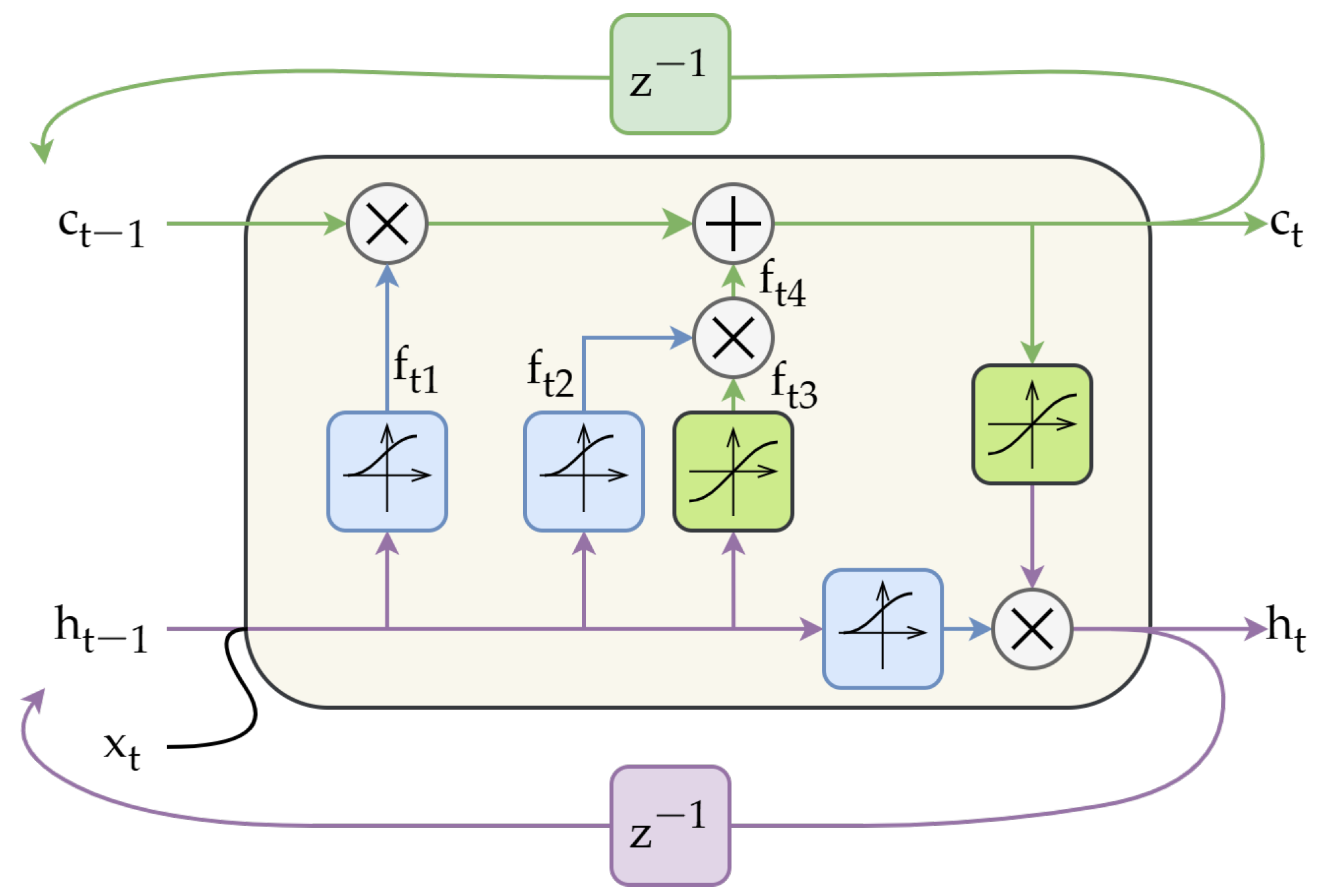
3. Deep Neural State Variables Estimators

The constant growth of technological requirements raises the need for more dynamic and versatile control solutions that can keep up with increasing maintenance and versatility demands. Due to the fact that electric motors feature high dynamics and durability, they are often implemented in many applications. However, the call for durability forces the need to minimize the occurrences of hypothetical drive system failures and breakdowns. Because electric motors constitute an excellent solution for many applications, they are often coupled with sophisticated machinery that they must control. To do so, a set of specified information about the current state of the machine needs to be delivered to the control loop. The demanded state–space variables are often measured using physical sensors (e.g., electric current, speed, or torque sensors). Mechanical sensors are the parts of the drive system that are the most likely to fail. In order to avoid the mentioned breakdowns, estimators of state–space variables constitute a common solution in the field of automation. Not only can they provide the ability of typical variable estimation (e.g., speed), but they are also in charge of approximating the unmeasurable state–space variables (e.g., stator/rotor flux). Thus, the issue of variable estimation is a mandatory point of each electric drive system.

The commonness of state–space variable estimation resulted in elaborating a variety of different models that can provide the desired information. The first category of such solutions is based on the mathematical description of the plant (e.g., state simulators). They are a basic mathematical copy of the controlled plant. As the control signal is passed on to the simulator input, the model produces an appropriate response similar to the one obtained with the real object. However, one of the biggest disadvantages of the state–space simulators is placed in their dynamic properties. It turns out that their dynamics are as high as the plant’s, which disqualifies them from being used in highly dynamic control loops. Thus, it raises a significant inconvenience in terms of controlling sophisticated drive systems (e.g., robust/adaptive control, object with time-varying parameters). The second group of tools used in state–space estimation is defined as State Observers. One of the biggest differences between the abovementioned solutions is the fact that State Observers can feature higher (and adjustable) response dynamics than the actual plant. The State Observers are mostly based on the Luenberger observer model, which is equipped with additional feedback (defined as a difference between the actual and estimated variable values). Moreover, in terms of variable estimation, Kalman filters are also a popular solution, suitable for signals with a high noise level. Despite the fact that each of the abovementioned structures provides satisfying quality, they are highly dependent on the set of tunable parameters that need to be properly adjusted to the controlled plant.

The second type of state–space variable estimation is based on shallow neural networks. Various research has shown that they can be considered an eligible tool in terms of their estimation properties. However, it has been proven that the form of the input vector has a significant influence on the quality of the estimation. Furthermore, shallow neural network structures are not a robust solution in terms of a significant change in the plant parameters. As the technology evolves, the availability of modern and highly efficient microprocessor units creates an opportunity to use deep-learning tools for the sake of state–space variable estimation, as they may deliver increased robustness and simplify the overall design/training process of the designed structure. Using deep-learning tools may also provide the ability to elaborate a state–space variables estimator prepared for different operating point conditions. Furthermore, due to the variety of different deep-learning components, deep neural estimators may also be useful concerning both the issues of signal estimation and filtering at the same time.

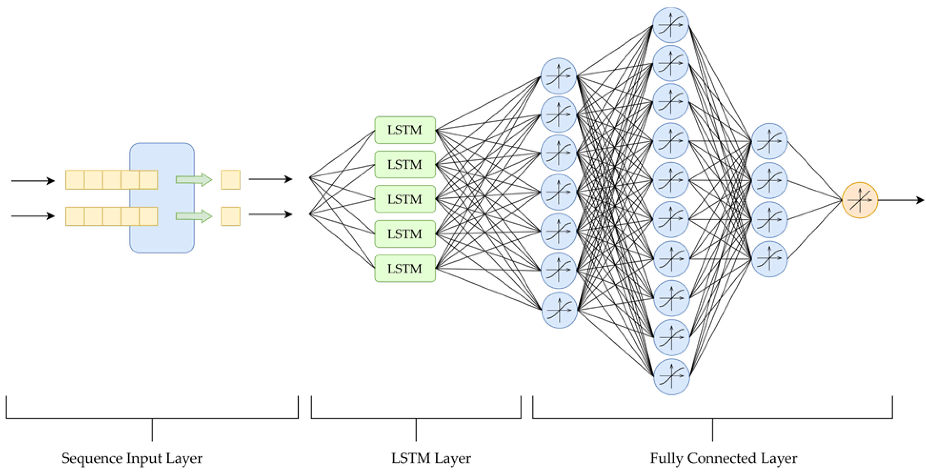
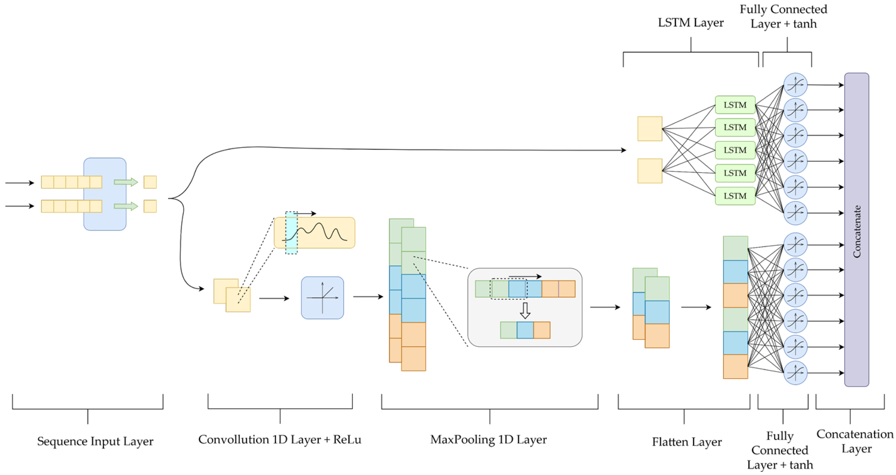
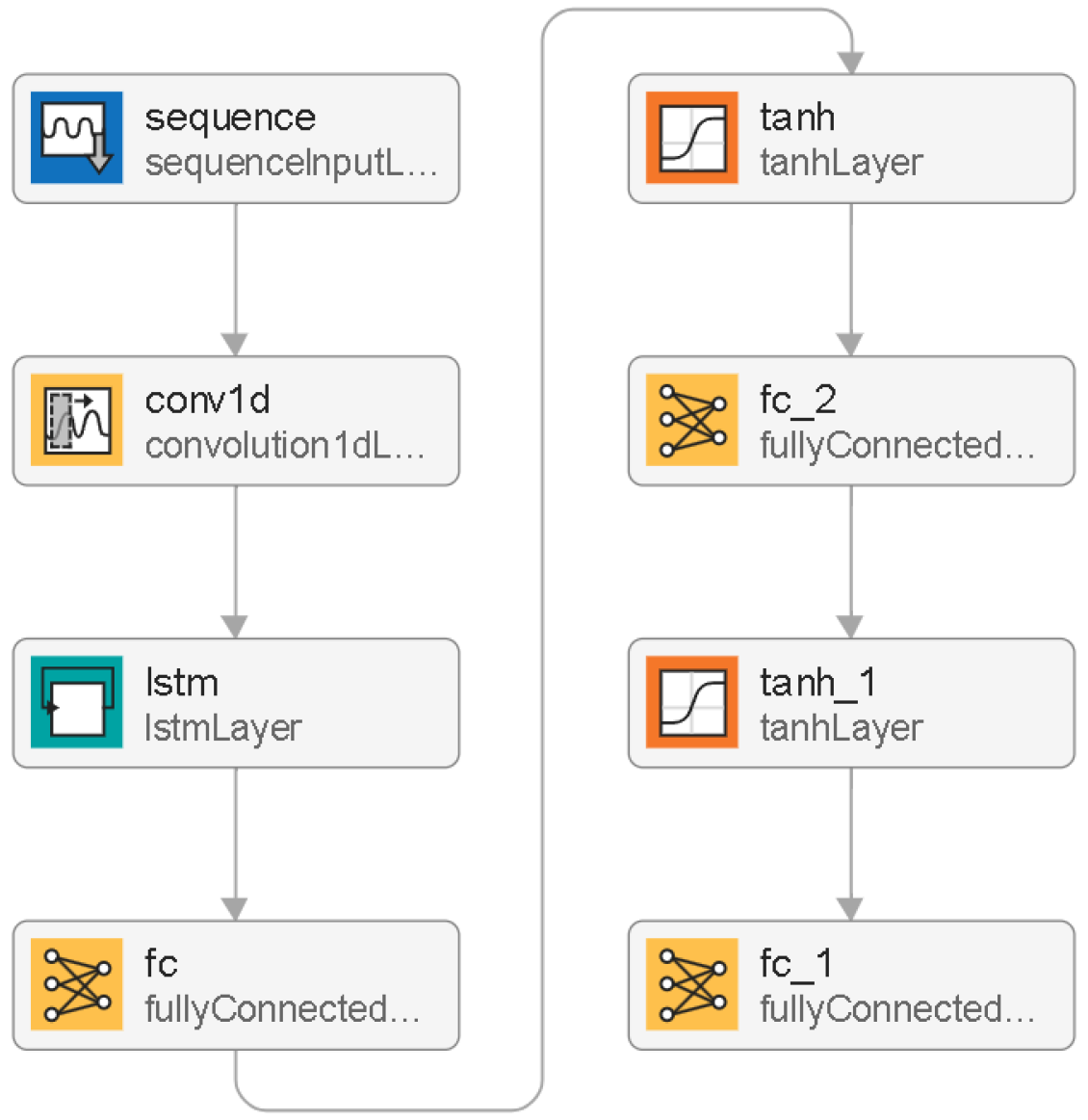
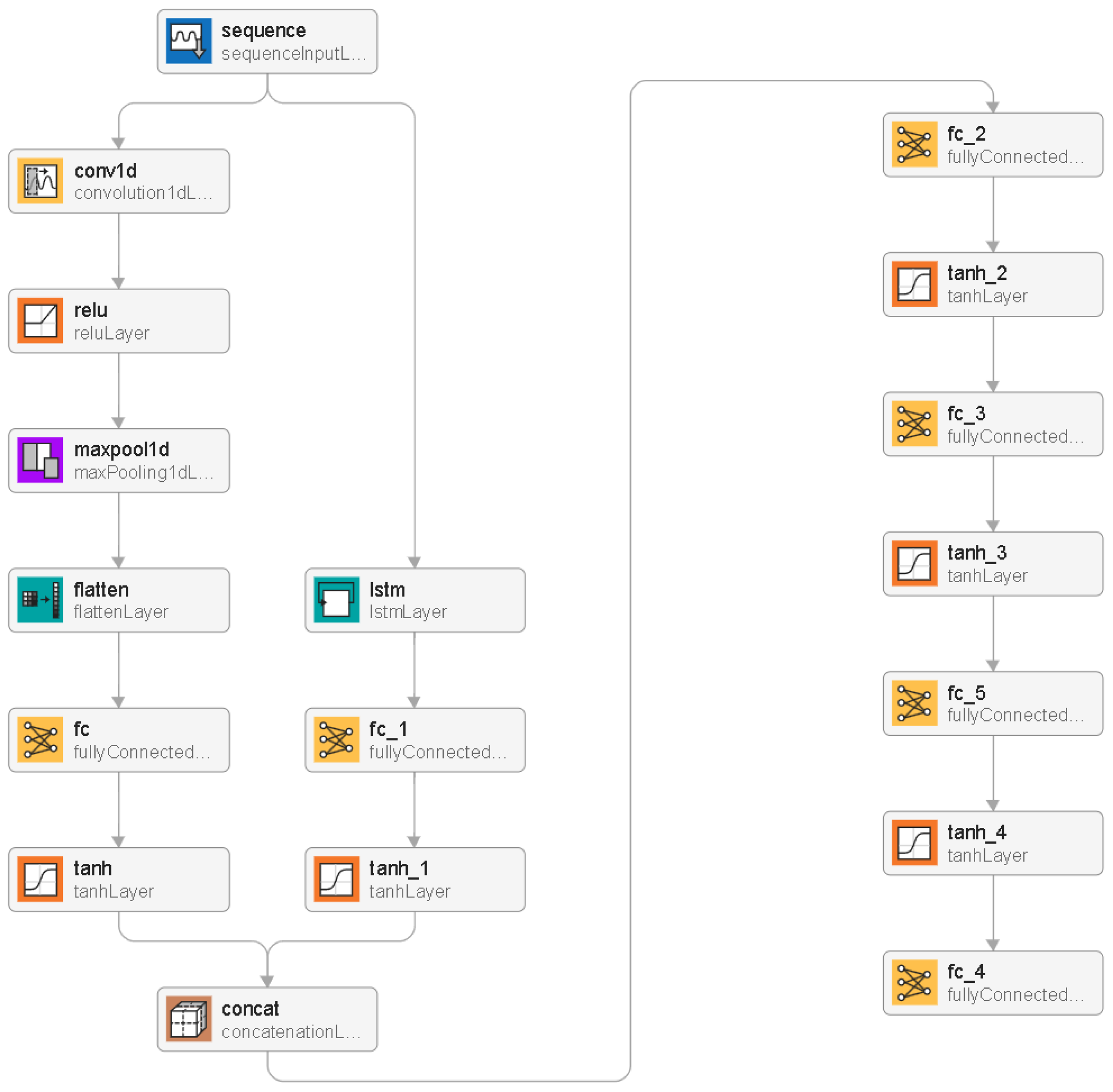
3.1. The Structure of the Neural Models

In this paper, authors focus on developing deep-learning models dedicated specifically to state–space variable estimation in a high dynamics system (i.e., an electric drive unit with a complex mechanical structure). The main point of the proposed solutions assumes the analysis of the way in which convolution and LSTM units affect the quality of the estimated signals. One of the crucial assumptions says that proposed neural models need to handle the estimation task in real time, as they need to be easily integrated with the main control loop of the drive in the form of additional system feedback.

The convolution operation constitutes an inseparable part of deep learning, which is widely used in image recognition applications. Its main purpose is to extract high-level features from the given image. The role of the Convolution operation is similar in terms of data series prediction tasks. It performs the product operation between two matrices: the given sequence-input data and the kernel. The role of the kernel (filter) is to slide across the entered data samples with a pre-defined stride and to extract key features of the signal. Then, the convolution layers are usually integrated with an activation function whose main role is to normalize the extracted feature map. For the sake of time-series data forecasting, a one-dimensional (1D) convolution is used since the entered data are a one-dimensional sequence input. The general idea of the 1D Convolution operation is presented in Figure 2.

The next stage of data processing in the network is called pooling. The main role of the pooling layer application is to reduce the size of the extracted feature map obtained during the convolution process. It is accomplished by decreasing the number of parameters in the input matrix. Two main kinds of pooling operation can be distinguished: maxpooling and average pooling. The maxpooling operation chooses the maximum value from the area embraced by the kernel, while the average pooling is based on calculating the average value from the same area. The purpose of running the pooling operation is to reduce the amount of conducted calculations, which affects the computational power required to execute the neural model. The main idea of Max Pooling is shown in Figure 3.

The field of neural networks offers a wide variety of different structures and techniques depending on the desired task. Recurrent Neural Networks can be considered an enormously essential network topology, especially useful for making predictions. The mentioned prevalence is also visible in data forecasting. However, the idea of a recurrent neural network assumes the presence of additional feedback placed within one hidden layer or between layers. In the case of a highly expanded neural model, the Exploding/Vanishing Gradient problem can be a huge concern. It turns out that the abovementioned additional feedback can make the gradient value exceed the tolerable level. Hence, the steps taken by the optimization algorithm during the training process are too large. Thus, the optimal set of parameters may never be found. One of the possible solutions to omit the described phenomenon is to limit the weight values and make them smaller than 1. Nevertheless, by doing so, the gradient becomes incredibly small, which also results in training difficulties. In order to tackle the problem of vanishing gradient value, the long short-term memory (LSTM) units are used.

The main assumption of the LSTM architecture states that data flow can be divided into two separate paths. By doing so, long-term memory can be separated from short-term memory. The described approach does not affect the overall long-term remembering capabilities and does not cause an enormously increasing/decreasing gradient issue. The basic LSTM unit scheme is presented in Figure 4.

Having analyzed the scheme presented above, two data paths can be distinguished: $c_t$—the green line representing the long-term memory path and $h_t$—the purple line representing the short-term memory. The upper line is barely affected by any operation as long-term memory needs to be retained. The overall data flow inside the LSTM unit can be divided into three stages called gates. The first one, the Forget Gate, is responsible for determining the percentage of long-term memory that is to be remembered by the LSTM unit. It involves the concatenation of the hidden state vector $h_{t-1}$ and the actual LSTM input $x_t$. The concatenated signals are passed through the sigmoid activation function. The mathematical description of the Forget Gate is presented in Equation (24):

$$f_{t1}=\sigma \left(f_{con}(h_{t-1},x_t)+b_{f1}\right),$$

(24)

where: $f_{t}1$—final Forget Gate equation, $b_{f1}$—bias, $f_{con}$—hidden state vector and input value concatenation, $\sigma$—sigmoid activation function, which can be presented with the Expression (25):

$$\sigma ={\displaystyle \frac{1}{1+e^{-x}}}.$$

(25)

The second stage of the data flow inside the LSTM unit is called the Input Gate. Its main purpose is to determine how to update to long-term memory data path. This is accomplished with the use of two parallel blocks. The first one calculates the percentage of the memory that is to be remembered. The mentioned coefficient is calculated using the sigmoid activation function and can be presented with the following Formula (26):

$$f_{t2}=\sigma \left(f_{con}(h_{t-1},x_t)+b_{f2}\right).$$

(26)

where $b_{f2}$—bias. The second block combines short-term memory and the actual input to create a potential long-term memory. This is carried out with the use of a hyperbolic tangent activation function and can be described as follows (27):

$$f_{t3}=tanh\left(f_{con}(h_{t-1},x_t)+b_{f3}\right).$$

(27)

where $b_{f3}$—bias and:

$$tanh={\displaystyle \frac{e^x-e^{-x}}{e^x+e^{-x}}}.$$

(28)

The final Input Gate equation can be written in the form of (29):

$$f_{t4}=f_{t2}·f_{t3}.$$

(29)

The final stage of the LSTM data flow is called the Output Gate. It updates the actual short-term memory with the new long-term memory value and determines the contribution of the actual short-term memory to its new value. The Output Gate equation can be presented in the form of (30):

$$h_t=\sigma \left(f_{con}(h_{t-1},x_t)+b_{f5}\right)·tanh{c}_t,$$

(30)

where $b_{f5}$—bias, $c_t$ is the final long-term memory value and can be presented as (31):

$$c_t=f_{t4}+f_{t1}·c_{t-1}.$$

(31)

The approach taken in the article is focused on creating preliminary research on the issue of deep-learning models dedicated specifically to state–space variable estimation. The whole research methodology is divided into three attempts. The first one involves the idea of creating a deep-learning structure similar to typical shallow neural estimators. However, to enhance the expected neural network response, one hidden layer is implemented in the form of LSTM units. By doing so, it is possible to compare the created network with conventional, well-known neural estimators. From this point on, in this article, the first network will be called the LSTM Neural Network. The general scheme of the abovementioned structure is presented in Figure 5.

The presented approach assumes that the network has four hidden layers: the first one consists of LSTM units, while the rest are equipped with hyperbolic tangent activation functions. The entrance of the network is accomplished with the use of a sequence-input layer, while the whole network is closed with the linear output neuron. In-depth analysis of network parameters is presented in

Table 1. The internal structure of the proposed LSTM Neural Network.

Name of the Layer	Input Size	Number of Hidden Neurons	Activation Function
Sequence Input Layer	2	—	—
LSTM Layer	2	12	sigmoid & tanh
Fully Connected Layer	12	24	tanh
Fully Connected Layer	24	32	tanh
Fully Connected Layer	32	16	tanh
Output Neuron	16	1	linear

,

Table 2. The internal structure of the proposed CNN Neural Network.

Name of the Layer	Input Size	Number of Filters	Number of Hidden Neurons	Activation Function
Sequence Input Layer	2	—	—	—
1-D Convolution Layer	2	16	—	—
LSTM Layer	16	—	32	sigmoid & tanh
Fully Connected Layer	32	—	48	tanh
Fully Connected Layer	48	—	16	tanh
Output Neuron	16	—	1	linear

and

Table 3. The internal structure of the proposed Parallel Neural Network.

Name of the Layer	Input Size	Number of Filters/Pool Size *	Number of Hidden Neurons	Activation Function
Sequence Input Layer	2	—	—	—
1-D Convolution Layer	2	16	—	ReLU
1-D MaxPooling Layer	16	2 *	—	—
Flatten Layer	—	—	—	—
Fully Connected Layer	16	—	24	tanh
LSTM Layer	2	—	12	sigmoid & tanh
Fully Connected Layer	12	—	24	tanh
Concatenation Layer	—	—	—	—
Fully Connected Layer	48	—	32	tanh
Fully Connected Layer	32	—	16	tanh
Fully Connected Layer	16	—	8	tanh
Output Neuron	8	—	1	linear

* Pool Size.

.

The second neural network proposed by the authors includes the convolution layer. Electric drive units feature a set of typical state–space variable transients. The convolution layer is implemented to discern the distinctive features of those signals. Hence, it makes it easier for the network to predict the transient of the estimated variable. For the sake of the following part of the research, the second network is named the CNN Neural Network, whose general topology is presented in Figure 6.

The CNN Neural Network is also made of 4 hidden layers. However, after the sequence-input layer, the one-dimensional convolution layer is applied. The second hidden layer is comprised of LSTM units. After being passed through the long short-term memory layer, the data are passed on to two Fully Connected Layers with hyperbolic tangent activation functions. The output of the network is accomplished with one linear neuron. Having conducted a detailed analysis of the CNN Neural Network topology, it can be observed that there is no activation function related to the convolution layer. In typical CNN Neural Networks, convolution layers are usually combined with a ReLU activation function, which is responsible for data regularization. Nonetheless, in the case of the CNN network used, the data normalization is accomplished inside the LSTM units. Hence, it is assumed that the additional activation function is not mandatory.

The proposed deep-learning neural models are expected to deliver a satisfying quality of the estimated state–space variables. However, small differences are expected. The LSTM Neural Network is more likely to keep up with sudden dynamic changes in the predicted value, as it can remember long-term interdependencies between particular plant variables more efficiently. Hence, LSTM neural networks are more suitable for dynamic time-series predictions and can recreate the model dynamics more accurately. On the other hand, the CNN Neural Network should pick up the general time-series tendencies, which should be noticeable, e.g., in the filtered steady-state transients. In order to combine the expected advantages of each neural model, the third approach is proposed.

The next neural network merges the advantages of both previously described models: the LSTM and CNN networks. In order to deliver the intact data flow in key sections of the proposed networks, it is assumed that the parallel data path needs to be applied. By doing so, the crucial parts of both the LSTM and Convolution networks are kept unbothered. They merge in the further part of the network. In order to keep the overall scheme of the proposed solution clear and transparent, it is divided into two main sections: Preliminary Data Processing—presented in Figure 7, and the Fully Connected Layer—shown in Figure 8.

Having analyzed the structure of the Parallel Neural Network (Figure 7), it can be seen that the convolution layer is not the same as it is in the case of the CNN Neural Network. The convolution layer is coupled together with the ReLU activation function. Then, after data normalization, the created feature map is passed on to the one-dimensional MaxPooling Layer, which reduces the size of the map. Then, after applying a Flatten Layer, the obtained data are transferred to the Fully Connected Layer with hyperbolic tangent activation functions.

For the sake of the research description, the neural network mentioned above will be named the Parallel Neural Network. Both parts of the network are merged in one common Concatenation Layer. Then, the obtained data are passed through two hidden layers with a hyperbolic tangent activation function. The output of the network is accomplished with the linear neuron.

3.2. The Design Procedure of Neural Estimators

The quality of the proposed deep-learning model response is strongly dependent on the conducted training process. In order to provide an eligible behavior of the estimator the set of the training data needs to include all vulnerable and specific states of the drive. It is mandatory to provide an insightful set of training data containing specific states of the drive for both speed and load torque directions. Furthermore, the appropriate selection of the training data form (both length and shape of the training vector) may visibly affect the final generalization capabilities of the network. Furthermore, the internal structure of the network (i.e., complexity, the number of hidden layers, and applied deep-learning tools) has a huge impact on the final estimation responsiveness. The main goal of the whole design procedure is to obtain the network that predicts all the drive states eligibly, especially considering circumstances for which it was not directly prepared. At this point of the research, the main task of the elaborated networks is to estimate the torsional torque of the two-mass drive system while having delivered the electromagnetic torque and the load machine speed value only. Thus, the form of the input vector in all three cases can be described as follows (32):

$${\mathbf{W}}_{\mathbf{1}}=[{\omega }_2\left(k\right),{\tau }_e\left(k\right)].$$

(32)

Moreover, to conduct a thorough analysis of the proposed structures, in some cases, an extended form of the input vector is used. It consists of the previous time samples of the main state variables (i.e., load machine speed and electromagnetic torque). The extended form of the input vector is presented below (33):

$${\mathbf{W}}_{\mathbf{1}}=[{\omega }_2\left(k\right),{\omega }_2(k-1),{\omega }_2(k-2),{\tau }_e\left(k\right),{\tau }_e(k-1),{\tau }_e(k-2)].$$

(33)

The output data used during the training process contains the torsional torque values, which correspond to the specific time samples of the input data. Thus, the main form of the output vector (for each of the three networks) can be presented with the following expression (34):

$$\mathbf{Y}={\tau }_t\left(k\right).$$

(34)

However, the further part of the conducted research involves the verification of the proposed neural model versatility. In this stage of the tests, it is mandatory to verify whether it is possible to estimate two state–space variables (i.e., the motor speed ${\omega }_1$ and torsional torque ${\tau }_t$) at once without applying any changes to the network structure. The only factor that differs described approach from the previous ones is the final form of the output vector, which can be presented as (35):

$$\mathbf{Y}=[{\omega }_1\left(k\right),{\tau }_t\left(k\right)].$$

(35)

The last stage of the estimator verification includes the different operating points. In terms of dynamic electric drive systems featuring high robustness/adaptation capabilities, it seems crucial to provide an estimation solution capable of ensuring a satisfying estimation quality without regard to actual circumstances. It is especially important in case the plant parameters become significantly changed (i.e., the mechanical time constant of the load machine increases). Thus, to supply the complete elaboration of the examined deep neural network estimators, their response will also be evaluated in case the mechanical time constant of the load machine increases 3 times (36):

$$T_2=3T_{2n}.$$

(36)

The internal structures of the proposed neural networks were selected experimentally based on the author’s experience and the minimal estimation error of the chosen state variables. During the verification process, the quality of the returned data series was taken into account. However, the necessity of real-time network deployment is a mandatory demand in terms of future electric drive control loop implementation. Thus, real-time execution was a crucial criterion during the final selection process of the proposed neural network architectures. At this point, it should be noted that for further real-time execution, the convolution filter size is restricted. That is because the micro-processing unit (calculating neural networks) will be supplied with one sample of a particular state variable each time step. In order to minimize mistakes caused by wrong data load and avoid using additional padding, the convolution filter size is limited to one. Each network was built with the use of the Deep Network Designer Tool (part of the Matlab/Simulink 2024b environment). The training process was carried out with the use of the Adam Optimizer algorithm (1200 epochs each with batch size set to 64). An in-depth analysis of the structure of consecutive networks is presented in Table 1, Table 2 and Table 3. The scheme of each network built in the Deep Network Designer tool is presented in Figure 9, Figure 10 and Figure 11.

The whole research process has been divided into three main sections. The first one contains simulation tests of the proposed deep-state-variables estimators (Section 4). Both the training and validation data sets are acquired from the simulation model created in the Matlab/Simulink environment. The control system attached to the plant model is presented in Figure 1. The second part of the evaluation is based on experimental verification. However, in the beginning, their offline execution is verified (Section 5.3). That being said, both the training and test data sets are acquired from the real laboratory test bench (including both input and output vectors). After collecting the data, proper vectors are prepared in a Matlab environment and loaded into the neural network. Nonetheless, despite the fact that the described approach clearly demonstrates the correctness of neural estimator response, it does not refer to the problem of real-time execution, which constitutes an underlying uncertainty in terms of its future usefulness. Hence, it is crucial to verify whether deep-learning-based neural estimators can be a feasible comprehensive solution ensuring eligible dynamics for single- and multivariable estimation tasks at different operational points.

4. Simulation Tests of the State Variables Estimators Based on Deep Neural Networks

According to the research methodology described in Section 3.2, the first stage of neural model verification is related to the simulation tests. The numerical model of the two-mass electric drive system is based on the state–space vector controller, thoroughly analyzed in Section 2. Its multivariable feedback, including motor speed, load machine speed, and torsional torque, constitutes a favorable control strategy. It ensures easy access to all required state variables. The numerical model of the two-mass motor system is accomplished using mathematical equations in the Laplace domain. Motor system parameters used in the experiments are presented in Section 5. In order to conduct a reliable training process, proper data sets are extracted. To adjust a variety of internal neural network parameters, the applied optimization (learning) algorithm requires different states of the drive.

It includes different steady-state reference speeds of the drive and ramp trajectory, forcing the drive to follow the speed change with strictly defined dynamics. The second variable defines the precise moments of additional attachment and detachment of the load torque equal to the nominal electromagnetic torque of the drive. The reference load signal controls the launch of the load machine. After conducting a training process, it is mandatory to validate the quality of the neural model response. To do so, a second dataset, presented in Figure 12, is created.

The first series of tests are conducted on each neural structure: LSTM, CNN, and Parallel Neural Network. The obtained results are shown in Figure 13, Figure 14 and Figure 15. Having analyzed the obtained results, it is noticeable that each of the presented neural estimators follows the actual torsional torque trajectory accurately. Nevertheless, the quality of the torsional torque estimation in the dynamic states of the drive is best predicted by the Parallel Neural Network. Comparing its response (Figure 15b) to similar attempts with LSTM and CNN structures (Figure 13b and Figure 14b) proves that the estimation error seems to be the smallest in the case of the Parallel Neural Network. There are also some inaccuracies visible in steady states that occurred after additional torque load attachment (Figure 13b–Figure 15b). However, the estimation error in the case of the abovementioned steady states is also the lowest for the Parallel Neural Network test.

In order to verify generalization properties, an additional test is performed. The main assumption of the extra attempt is to verify the network responses, including those states of the drive that were not taken into account during the training process. The reference speed, the load torque, and the obtained results transients are presented in Figure 16 and Figure 17.

After conducting a thorough analysis of estimated transients, it is noticeable that there are some visible differences between the obtained predictions. In previous attempts, each network has eligible dynamics and response quality. The achieved network responses differ from each other mainly in steady states. However, by supplying the input of each network with data vectors containing specific states of the drive (neural networks were not trained for, i.e., sudden speed-direction returns), neural estimators start to provide distinct estimations. The torsional torque transients presented in Figure 16b and Figure 17a show that the behavior of the LSTM and CNN Neural Networks is not sufficient. The peaks, visible on the negative side of the Y-axis, do not keep up with the actual value of the state variable. However, the first two structures respond eligibly in all steady states (i.e., after load torque attachment). However, the overall quality of the response is not negligible. On the other hand, the analysis of the Parallel Neural Network behavior (Figure 17b) proves its higher robustness on a variety of drive states for which it was not prepared. The obtained torsional torque transients keep up with sudden, high-value peaks. Unfortunately, the presented behavior does not contain as good a steady-state estimation quality as it was during the first two attempts. However, in this particular case, the acquired inaccuracies are negligible. The simulation tests conducted clearly prove that the use of the most complex deep neural network guarantees the best prediction quality in the case of unexpected situations that were not directly included in the training process. Knowing that the response of the Parallel estimator is eligible, the next step (verification on data from the experimental test bench) can be performed.

5. Hardware Implementation of the Neural Models Applied for Signals of Two-Mass System Estimation

According to the overall research plan described in Section 3.2, the next stage of the evaluation of the deep neural estimators is focused on the real hardware implementation of the networks. However, the following section is divided into two stages. The first one contains the offline execution of the neural networks. What it means is that the input vector data are acquired from the laboratory test bench during the drive operation. It is also noteworthy that for the sake of all experimental tests, each neural network has been trained from scratch using experimental data. What is means is that the noise and other disturbances are taken into account in the training data sets. Then, neural models are supplied with collected data and executed in Matlab. The main purpose of the first stage is to verify the correctness of deep estimators with real, non-hermetic, noised data. The course of this stage is comprehensively presented in Section 5.3. The second stage then involves what the authors call real-time network execution. This means that the neural estimators are calculated during the work of the drive. This stage of the tests constitutes a mandatory elaboration of the whole deep-learning estimation design procedure. The electric drive control issue arises mainly during highly dynamic states. Thus, in order to make the proposed neural estimators utilizable, a real-time execution ensuring correct, anticipated response is a crucial affair.

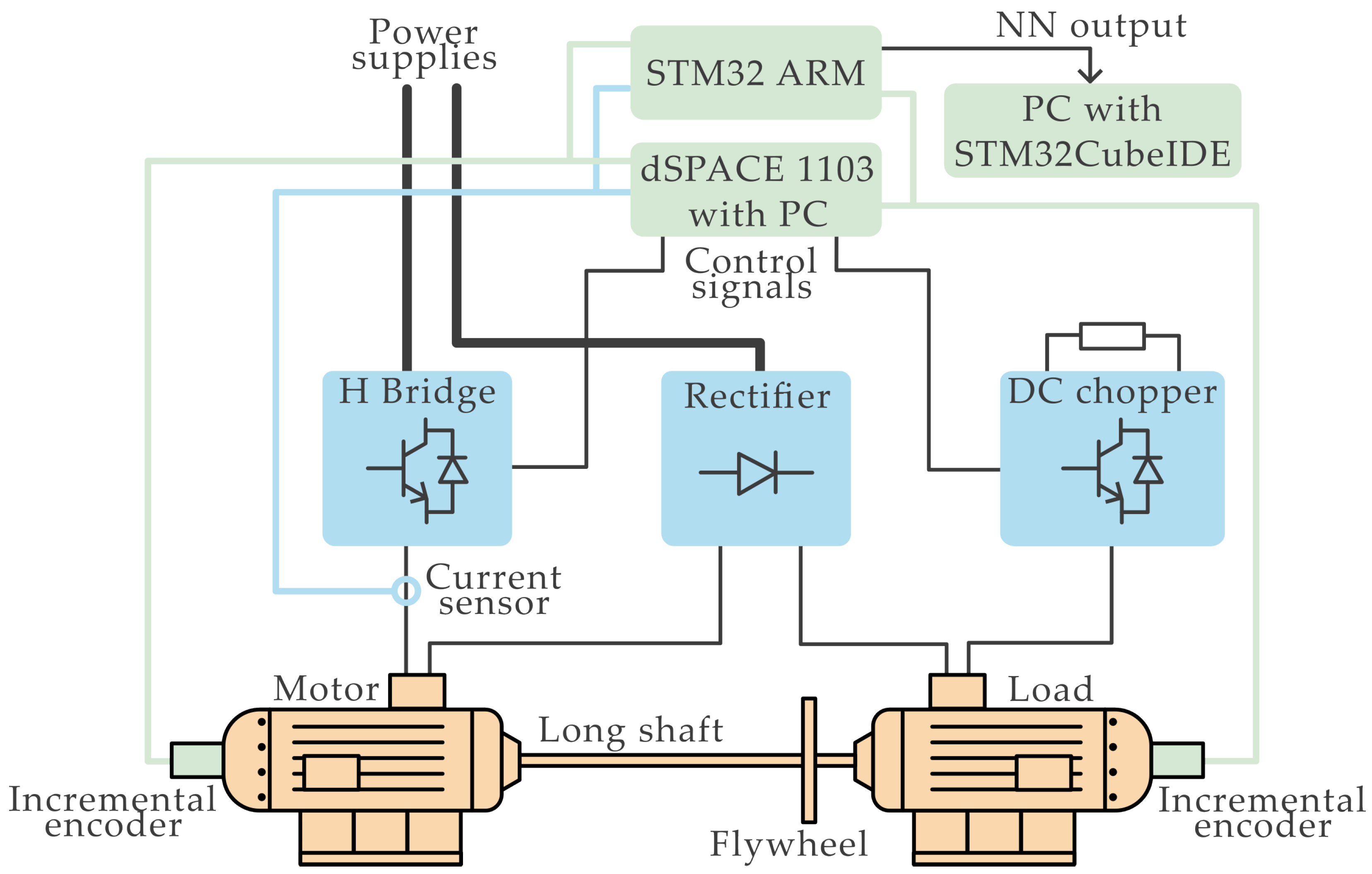
5.1. The Laboratory Equipment

The laboratory setup used in the research is based on two 0.5 kW DC motors. Electric machines are coupled with a long and flexible shaft. Its role is to introduce additional elasticity and torsional vibrations to the system since it simulates a variety of complex real-life drive systems equipped with a sophisticated mechanical structure. Moreover, the presented test bench gives the possibility of forcing a significant change in the plant parameters. It is accomplished with the help of additional flywheel weight attached to the load machine shaft. The speed of both motors is measured using incremental encoders. The whole control system is numerically executed on the dSPACE 1103 Rapid Prototyping System (dSPACE GmbH, Paderborn, Germany). The main processor receives both speeds and current feedback and, after performing a set of mathematical calculations, returns the final control signal. The control output is then passed on to the Power Converter, which powers the controlled motor directly. Detailed parameters of the laboratory stand are collected in

Table 4. Basic parameters of the used experimental setup.

Parameter	Value	Symbol
Nominal Motor Power	500 W	$P_N$
Nominal Angular Speed	1450 RPM	$n_N$
Nominal Encoder Resolution	36,000 p./rev.	—
D.C. Motor Mechanical Time Constant	0.203 s	$T_1$
D.C. Load Machine Mechanical Time Constant	0.285 s	$T_2$
Elastic Shaft Mechanical Time Constant	0.0026 s	$T_c$
dSPACE DSP sample time	0.0005 s	$t_{s-dspace}$

.

5.2. Low-Cost Implementation of the Deep Neural Network

The correctness of the real-time execution of the proposed deep-learning neural network estimators constitutes an undeniable issue. However, a wide variety of scientific research is often deployed on expensive, non-easily accessible rapid prototyping systems often equipped with high-performance digital signal processors. This approach ensures high efficiency of the elaborated applications but is not a reliable solution. Thus, in order to conduct a comprehensive real-time verification, it is assumed that proposed deep-learning models are numerically executed on the ARM microcontroller included in the STM32 Nucleo F767Zi Development Board (ST Microelectronics, Geneve, Switzerland). The proposed device is a low-cost floating-point unit that ensures relatively high numerical performance. It supports DSP, double- and single-precision data-processing instruction sets. Furthermore, having combined high numerical capabilities of the ARM core with its low, maximum power consumption (approximately 1.3 W), the Nucleo board is considered a perfect tool for the presented task. Moreover, the additional prevalence of the proposed device is the fact that it supports modern, deep-learning Matlab libraries, which significantly simplifies the whole development and deployment process. At this point, it is mandatory to assess the resource utilization of the Nucleo board. To objectively analyze the amount of used memory two cases can be distinguished. The first one involves the network execution only (without input data supply, communication protocol configuration, etc.), which uses 0.08 MB (Parallel Neural Network) of flash memory. The second case concerns the full program execution, which uses 0.46 MB of flash memory. Considering the fact that the maximum available flash memory capacity is 2 MB, the abovementioned cases use $4\%$ and $23\%$, respectively. At this point, it is worth emphasizing that the ARM processor does not participate in the electric drive control process. It works outside the main control path. It receives the speed and electromagnetic torque values, which are transferred with the use of the digital communication protocol UART. After receiving the data samples in each time step, it supplies the neural network input with actual speed and torque values regarding the input vector shape (Equation (32)). The general scheme of the laboratory equipment is presented in Figure 18.

The dSPACE’s digital signal processor works with the time step included in Table 4, which is equal to $t_{s-dspace}=0.0005$ s. The main idea behind real-time execution is to keep the consistency between the time in the ARM processor and in real-life. Thus, it is assumed that the sampling time of the STM32 processor is equal to $t_{s-stm32}=0.005$ s. The digital signal processor, included in the dSPACE device, generates the data send request every $t_{s-stm32}$ period. The ARM processor included in the Nucleo board handles the UART interrupt triggered by the dSPACE system and receives the sent speed and torque samples, which are then supplied to the executed neural network. The Nucleo Development board is controlled with an additional PC equipped with a Matlab/Simulink environment. The data network response is supervised in real time with the use of the Simulink Data Inspector tool. The detailed picture of the laboratory setup is presented in Figure 19.

5.3. Calculations Based on the Real Data

The order of examination of the proposed neural estimators is the same as in the chapter on simulation tests (Section 4). The reference signal transients are similar to those presented in Figure 16a. That being said, the electric drive system makes four sudden speed-direction returns. During two of them, the additional, temporary load torque attachment occurs. The first network to verify is the LSTM neural estimator. The obtained results are presented in Figure 20. The overall estimated torsional torque transient is shown in Figure 20a, while the zoom-in showing the dynamic states of the drive and the additional load torque attachment moment in detail is presented in Figure 20b.

Having taken a closer look at the torsional torque transients in Figure 20a,b, it can be noticed that the first network (LSTM) correctly estimates the desired variable. However, some inaccuracies are visible. The quality of the estimation in steady state (after additional load torque attachment, Figure 20b) is not sufficient. Moreover, the examined network does not properly reproduce the torsional torque in the dynamic state of the drive at time t = 15–16 s. The obtained results are generally correct, but in-depth analysis exposes some inaccuracies. The next verified neural network is a CNN structure. The results obtained during the next test are presented in Figure 21a,b.

The results presented above demonstrate that the quality of the CNN neural estimator is similar to the LSTM structure. The torsional torque data series is correct in general. However, a closer analysis of transients presented in Figure 21a indicates that the mean value in the negative steady state of the drive (e.g., t = 16–20 s) features unwanted offset. Furthermore, the network response in the steady state of the drive, shown in Figure 21b at t = 12–13 s, differs significantly from the actual torsional torque transient. Furthermore, the dynamic state of the drive (t = 15–15.5 s) does not follow the actual variable transient accurately either. The overall quality of the CNN Neural Network response is eligible, but it features some inaccuracies as well as the LSTM Neural Network. Hence, the further part of the experimental verification involves the Parallel Neural Network examination.

For the sake of thorough analysis of different Parallel Neural Network variants, its name in further attempts is extended with input/output ratio (e.g., in-out [2-1] denotes the Parallel Neural Network with two inputs and one output). The results of the torsional torque estimation obtained with the execution of the Parallel Neural Network are presented in Figure 22.

A detailed analysis can show that the quality of the Parallel estimator response is the best among all three examined structures. It estimates the correct steady-state torsional torque value, which is filtered but does not contain any mean value offset (Figure 22a). The steady-state prediction in case of additional load torque attachment is the most accurate as well (Figure 22b). Moreover, the presented transients converge with the actual torsional torque value in dynamic states of the drive (i.e., speed return peaks, t = 10–10.5 s, t = 15–15.5 s) accurately. Having concluded the overall Parallel Neural Network response, it can be stated that its quality seems the most satisfying.

Having obtained eligible results with each of the proposed structures, an additional stage of the evaluation involves the analysis of multivariable estimation. To do so, a Parallel Neural Network is taken. However, in this case, the output vector is presented with Equation (35). Hence, the only change in the network structure concerns the number of linear output neurons, which is equal to 2. The described attempt is to evaluate whether deep-learning neural networks are capable of handling multivariable estimation without changing their internal structure. The obtained results are presented in Figure 23 and Figure 24.

The examination of the presented results demonstrates that the Parallel Neural Network constitutes a promising base in terms of multivariable estimation. The estimated speed value follows the actual trajectory accurately. However, after a closer look at the speed transient shown in Figure 23b, it is noted that a small estimation error is visible after the additional attachment of the load torque (t = 12–13 s). The quality of the estimated torsional torque transient is satisfying. Nevertheless, a small difference in the estimated variable amplitude can be seen between the positive and negative steady states (Figure 24a). Visible inaccuracies can be caused by the same training time because it is used in the case of early tested networks. However, the overall estimation quality is eligible and proves the capability of multivariable estimation without the necessity of changing the internal network structure.

The next stage of the multivariable estimation network test verifies the impact of the extended input vector on the predicted data series. The described solution used to be an efficient way to increase the accuracy of the shallow neural network estimation, which has been proven in [45]. To do so, the input vector takes the form described with Equation (33). To evaluate the actual extended input vector impact, all training process parameters remain the same. The results obtained are presented in Figure 25 and Figure 26.

The insightful observation of estimated speed transients demonstrates that the extended input vector emphasizes the unwanted noise peaks, which occur in the steady states of the drive (e.g., Figure 25a—t = 0–5 s, Figure 25b). However, the estimation error that occurs after additional attachment of the load torque (Figure 25b—t = 12–13 s) does not disappear. Furthermore, comparing the estimated transients of torsional torque obtained during this and previous attempts (Figure 23 and Figure 26) also highlights that the quality of the estimated variable does not improve after applying the extended input vector. Thus, the conducted attempt can be concluded with the fact that using the extended input vector form combined with deep-learning techniques in neural network estimation does not constitute an effective way to increase the quality of the predicted time-series.

5.4. Experimental Tests

The presented experimental tests section is a crucial part of the entire research evaluation. The main purpose of state-variables estimators is to include them in the highly dynamic control path. To fulfill the real-time demands of the control system, it is mandatory to execute the elaborated neural estimator with no delays regarding a real-time elapse. The correctness and validity of the proposed deep neural estimators have been proven in Section 4 and Section 5.3. The additional impediment of the verified approach is a time step difference described in Section 5.2. The sampling period of the Nucleo board is ten times bigger than the dSPACE time step. Hence, neural estimators will be supplied with incomplete input data. At this point, the authors endeavored to perform neural networks used in earlier tests. However, after a series of underperformed tests it turned out that all the networks did not converge accurately with the actual torsional torque transient. The predicted signal did not match the actual variable during rapid torque peaks. Thus, it was mandatory to apply the downsampling technique. The main purpose of the engaged solution is to produce a discrete approximation of the measured sequence data, which would be obtained if the dSPACE processor worked with a longer time step. By doing so, not only is the amount of training data reduced, but transients of the acquired time-series are adjusted to the ARM processor working with a lower sampling rate. It is a common strategy that corrects unbalanced data and improves the final model performance. The methodology of this part of the test is the same as in previous sections. The obtained results for each of the three examined structures (LSTM, CNN, Parallel [2-1], and Parallel [2-2] networks) are presented in Figure 27, Figure 28, Figure 29, Figure 30 and Figure 31.

The results of the real-time network execution confirm the validity of the proposed deep neural network estimators. In addition, in each of the presented cases (especially for LSTM and CNN Neural Networks), the transients obtained are even more accurate than those obtained in offline attempts. The quality of estimated state–space variables in the case of multivariable estimation (Figure 30 and Figure 31) satisfies the quality and dynamic requirements. However, due to the lack of significant differences between the behavior of the networks during real-time execution, it is decided to verify the convergence of the network if the plant parameters change. To do so, the authors decide to change the mechanical time constant of the plant (using the flywheel described in Section 5.1). The implemented time constant increase is accomplished according to Equation (36). It seems noteworthy to emphasize the importance of this part of the tests. Not only does it verify the applicability of the elaborated networks, but it also confronts their behavior with an uncommon state of the drive (not included during the training process). The obtained results for LSTM, CNN, and Parallel [2-1] neural estimators are presented in Figure 32, Figure 33 and Figure 34, respectively.

The observations of the estimated transients highlight significant differences between the proposed networks. Having taken a closer look at the torsional torque predicted by the LSTM Neural Network (Figure 32a), huge inaccuracies are visible. Despite the fact that the network tries to keep up with the high dynamic peaks, it is clearly noticeable that the network output is delayed (Figure 32b). However, it only happens for the positive torsional torque value. On the negative side, the estimated torque features an enormous error, which is unacceptable.

The transients produced by the CNN Neural Network shown in Figure 33 are even worse. The first significant fault in the predicted data is visible in Figure 33a (t = 2–3 s). It is visible that the output of the network starts to fluctuate and does not converge with the actual torsional torque value. Furthermore, the analysis of the dynamic states, shown in Figure 33b, presents that the estimated variable does not reach the top of the occurred peaks.

The estimated variable features similar inconveniences in terms of the Parallel [2-1] network (Figure 34). The neural model response might be acceptable for positive torsional torque peaks (Figure 34b). However, the estimator output does not provide a precise estimation quality for negative values. Thus, referring to previously conducted positively evaluated tests, an additional attempt is made. It assumes the extension of the training data, which involves the behavior of the system when the mechanical time constant is increased. By doing so, it is possible to assess each network, assuming its estimation ability for different operational points and real-time execution. The acquired estimation transients are presented in Figure 35, Figure 36 and Figure 37.

After including the increased load machine inertia in the training dataset, the obtained results feature very similar dynamics. Comparison of the transients shown in Figure 35, Figure 36 and Figure 37 proves that each network responds eligibly, but does not allow any detailed observations. To do so, an additional comparison is shown in Figure 38 and Figure 39. To increase the transparency of the chart, the Parallel Neural Network transient color is changed.

The final comparison proves that each of the proposed structures can be adjusted to more than one operational point at once. A zoom-in, showing the start-up moment, depicts the small differences between the networks. It can be noticed that the overshoot of the estimated value is smaller in the case of the Parallel Neural Network. The oscillations in the steady state of the drive after additional load torque attachment (Figure 39a) for the CNN Neural Network are not acceptable. The analysis of the zoom-in to one of the next speed returns (Figure 39b) also shows that the quality of each neural estimator is satisfying. To carry out an objective comparison of the proposed estimators, it is mandatory to apply an estimation error calculation. It is defined by the following mathematical expression:

$$E_r={\displaystyle \frac{1}{N}}\left(\sum _{i=1}^N\mid x_i-\widehat{x_i}\mid \right)·100\%,$$

(37)

where: $x_i,\widehat{x_i}$—real and estimated value, N—number of samples. The consecutive error values are correlated in

Table 5. Estimation errors for increased mechanical time constant.

Neural Network Type	${\mathit{E}}_{\mathit{r}}$ for ${\mathit{T}}_2=3{\mathit{T}}_{2\mathit{n}}$ Not Included in the Training Process	${\mathit{E}}_{\mathit{r}}$ for ${\mathit{T}}_2=3{\mathit{T}}_{2\mathit{n}}$ Included in the Training Process
LSTM Neural Estimator	9.09%	4.04%
CNN Neural Estimator	9.10%	4.00%
Parallel [2-1] Neural Estimator	8.36%	3.92%

Bold emphasizes the lowest values.

.

The collected error values also prove that the Parallel Neural Estimator features the best results among all three proposed neural estimators. Despite the fact that the differences may not seem significant (e.g., between CNN and Parallel Estimator for $T_2=3T_{2n}$ included in the training process), the overall estimated variable transient is not acceptable for the CNN estimator. It is caused by rapid fluctuations right after the first load torque attachment.

To compare each network’s resilience to significant changes in the plant parameters, an estimation error for the nominal plant is correlated with an estimation error increase. The increase in the estimation error is defined as a difference between $E_r$ for $T_2=3T_{2n}$ not included in the training process and $E_r$ for $T_2=T_{2n}$. The error calculations for the nominal plant parameters are based on transients obtained during real-time execution and are shown in Figure 27, Figure 28 and Figure 29. The proposed factor objectively evaluates the robustness of each network. The calculated factors are collected in

Table 6. Estimation errors for the nominal object parameter.

Neural Network Type	${\mathit{E}}_{\mathit{r}}$ for ${\mathit{T}}_2={\mathit{T}}_{2\mathit{n}}$ Not Included in the Training Process	${\mathit{E}}_{\mathit{r}}$ Increase Factor
LSTM Neural Estimator	2.05%	7.04%
CNN Neural Estimator	2.02%	7.08%
Parallel [2-1] Neural Estimator	2.07%	6.29%

Bold emphasizes the lowest value.

.

The analysis of the estimation error for the nominal plant parameters shows that the differences in estimator quality are negligible. The Parallel Neural Network, despite having the largest estimation error for nominal plant parameters, features the smoothest variable transients. It does not have any offset and converges the actual value the same way in different dynamic and steady states of the drive. The most important insight is related to sudden changes in plant parameters, which may occur in a real-life scenario. The Parallel [2-1] Estimator features the smallest increase in estimation error in terms of sudden circumstances that were not included during the training process. Each of the proposed networks works accurately during real-time execution.

6. Concluding Remarks

The paper analyses the applicability of deep-learning methods to estimate the torsional torque in electric drive systems. The performance of three deep neural networks is evaluated offline using simulation and experimental data. The models are also implemented on an ARM processor to verify their real-time operation on a low-cost device. The main contribution of the article lies in the proposed deep neural model with dual convolution-LSTM parallel data processing. The proposed approach combines the advantages of two structures: filtering and pattern recognition offered by convolutional layers and a better reaction to dynamic occurrences provided by the LSTM. The conclusions that can be drawn from the presented research results are summarized below.

• The main concept of the article is to verify whether deep-learning tools can enhance the versatility of neural estimators. The main points of concern include the reaction of the created networks to varying plant parameters and different operating points, quickness of response to dynamic states, and simultaneous additional benefits, e.g., filtering out white noise from the sensor signals.
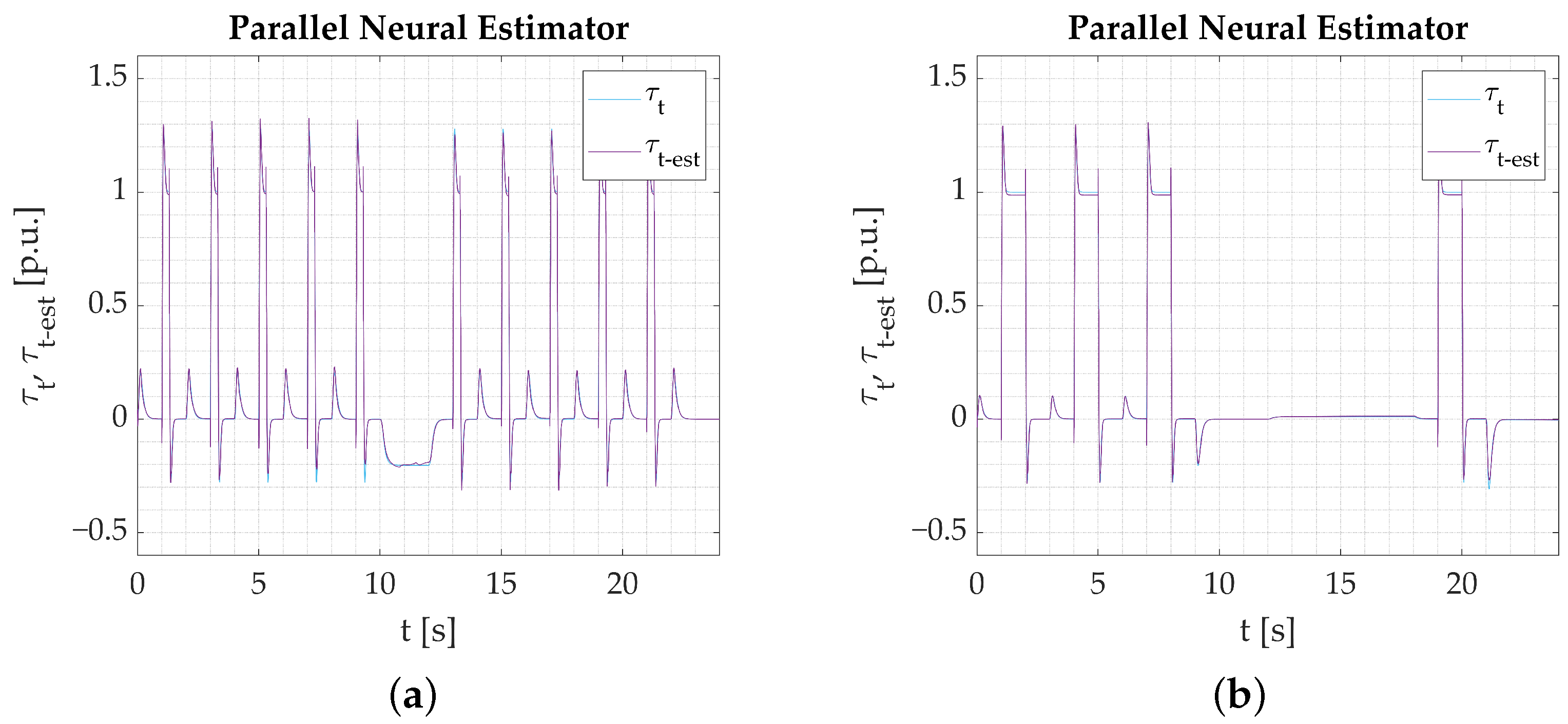
• Numerical studies serve as an initial stage of verification. The results help distinguish the networks’ tendencies and capabilities, but the main focus is put on the possibility of their application in programmable devices. Simulations show that the proposed Parallel neural model is eligible based on its estimation performance. The results are not substantially better than what could be expected from shallow neural networks. However, as stated earlier, at this stage, the most important information is that the model is eligible for application.
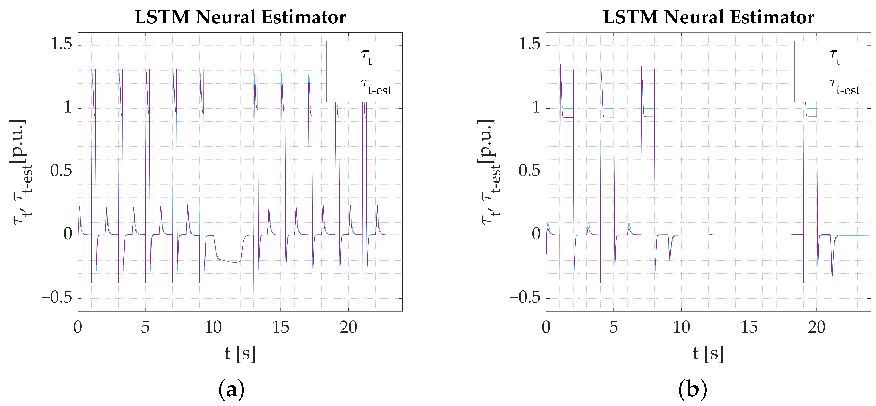
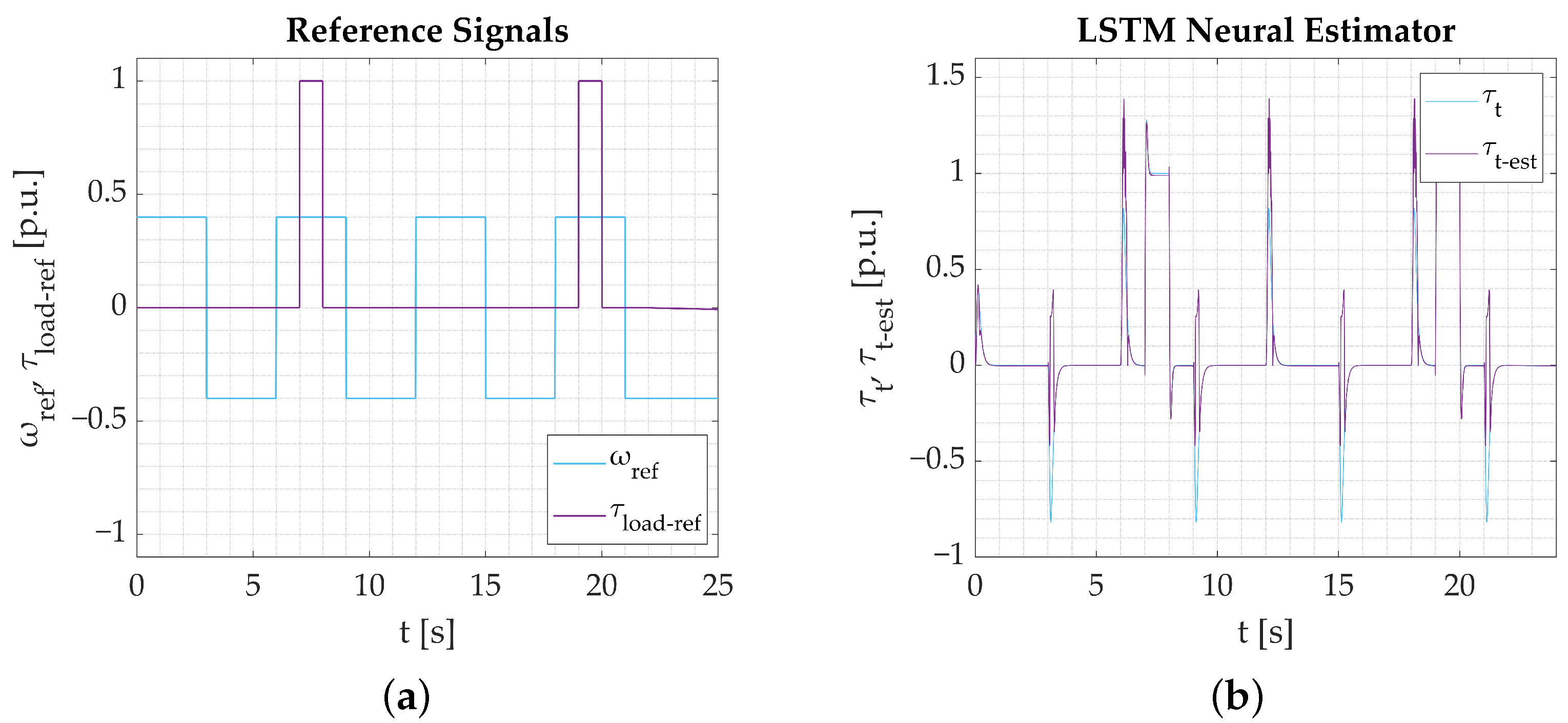
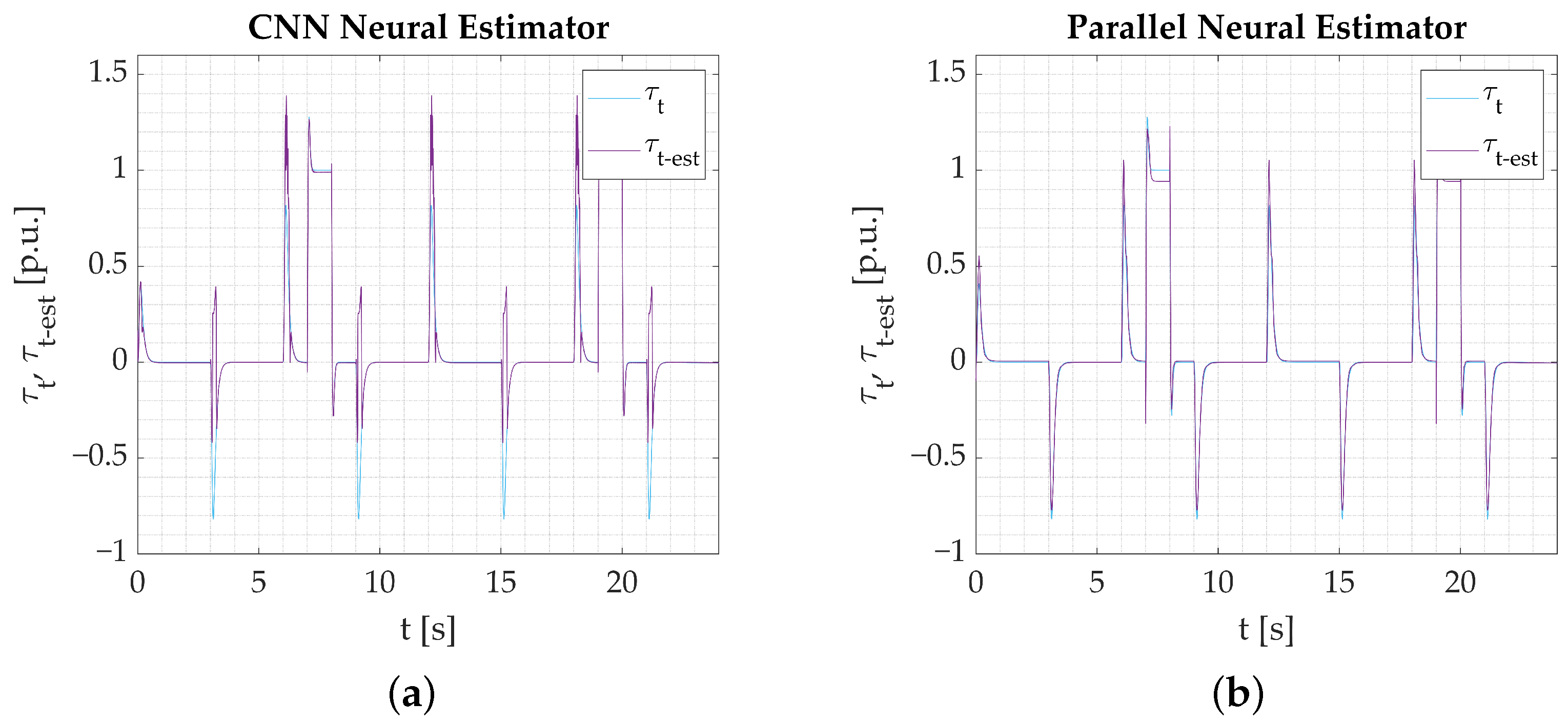
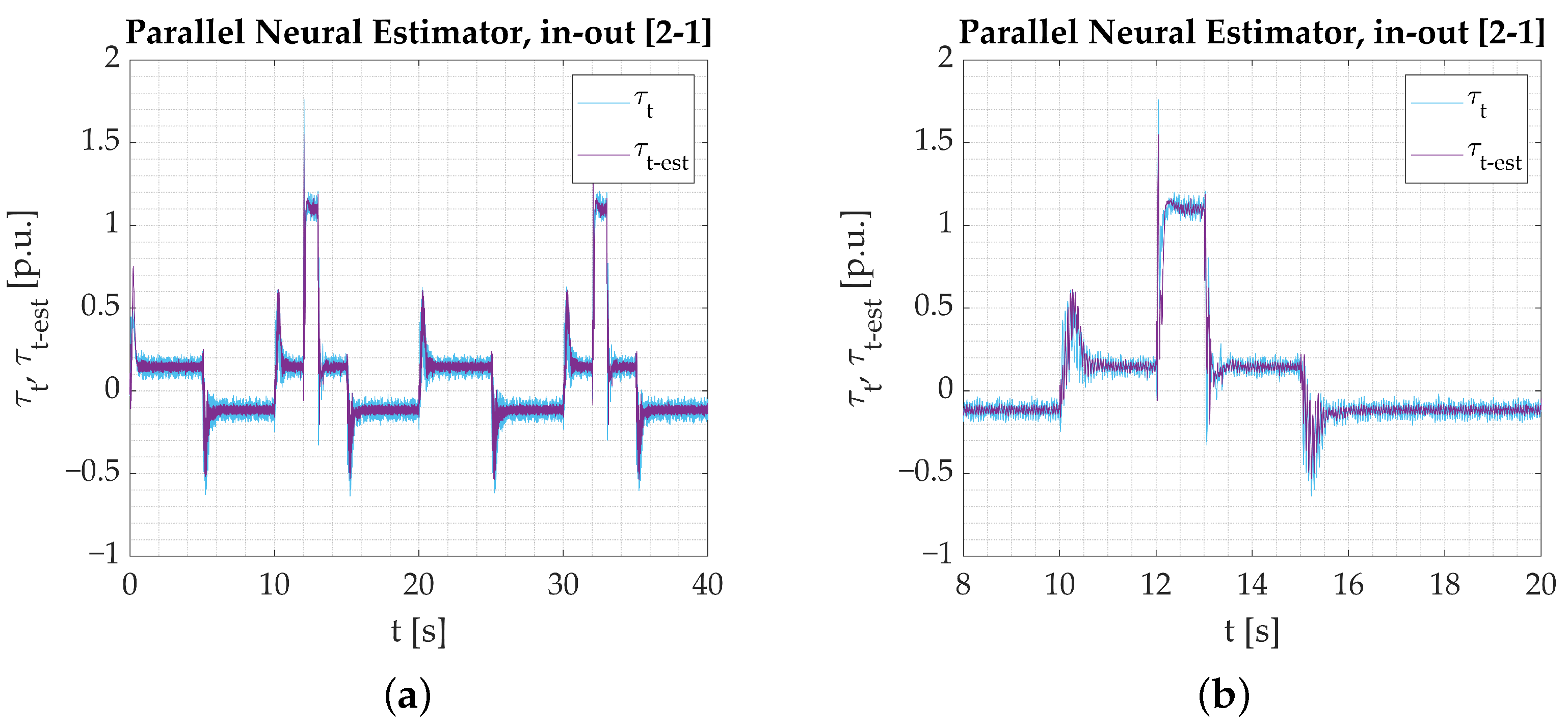
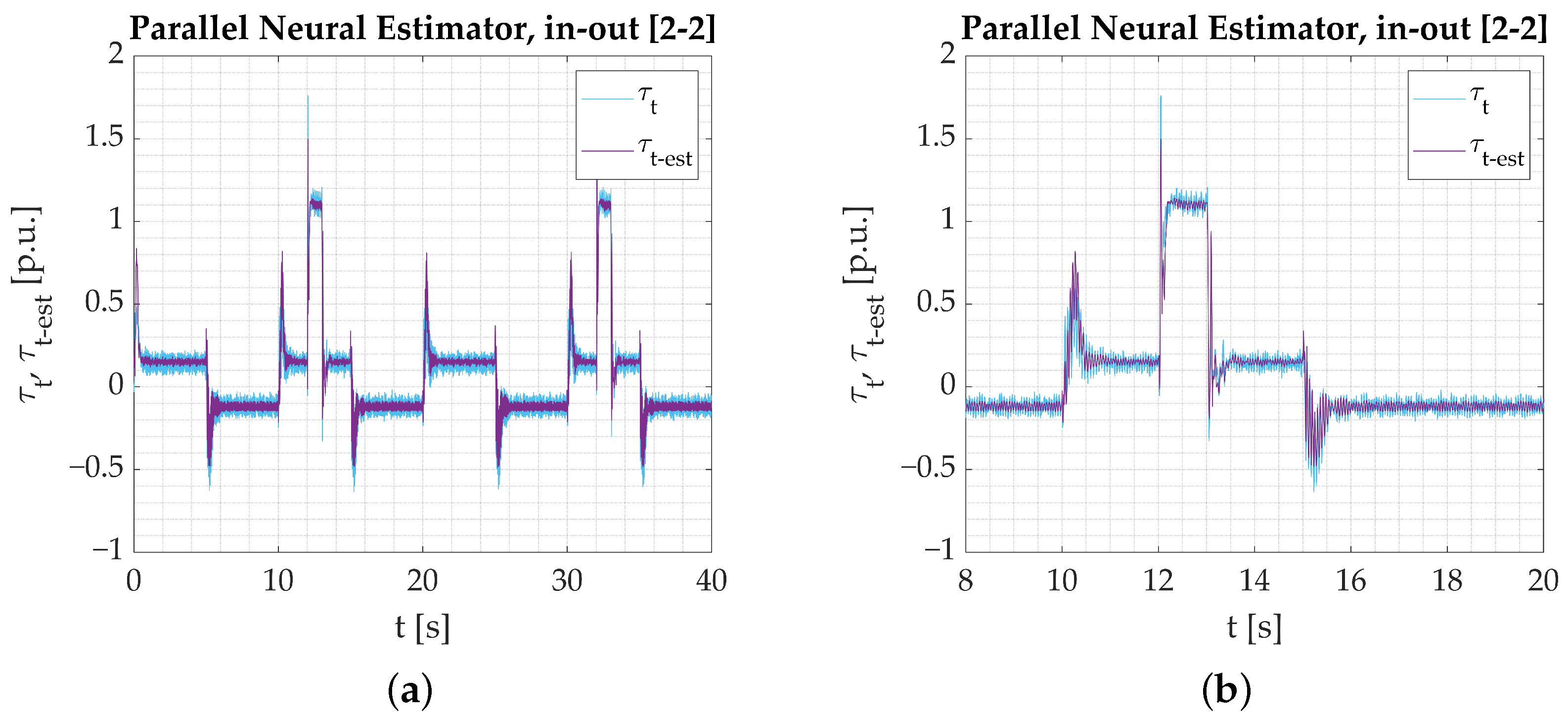
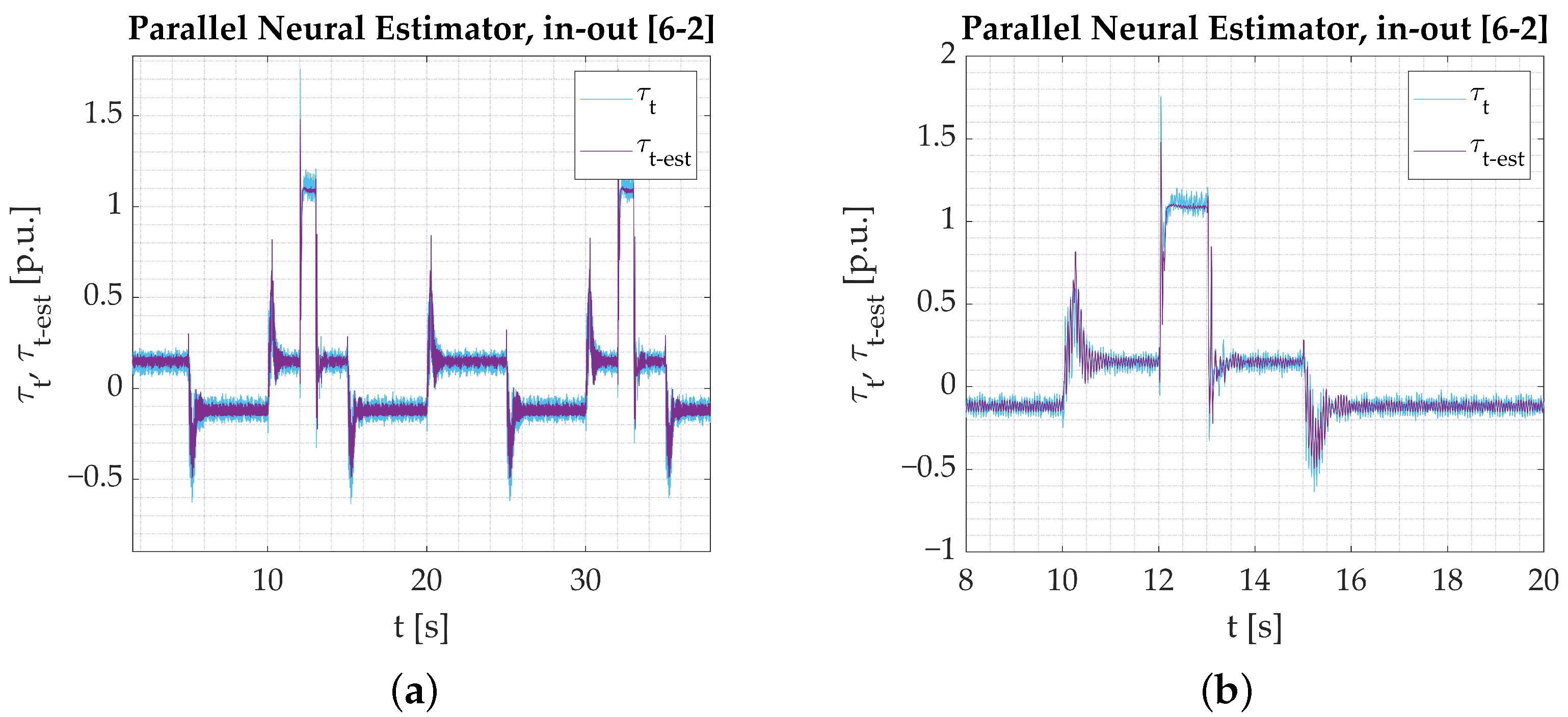
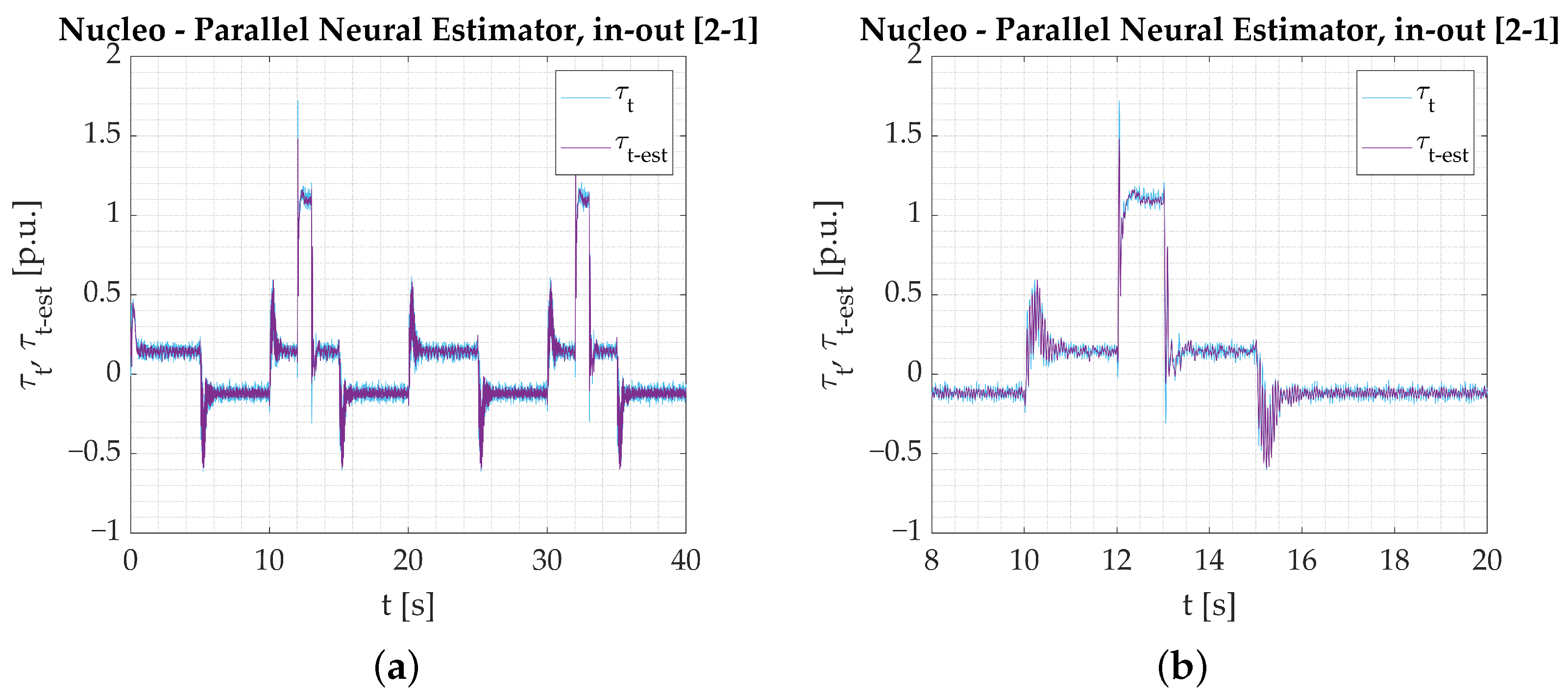
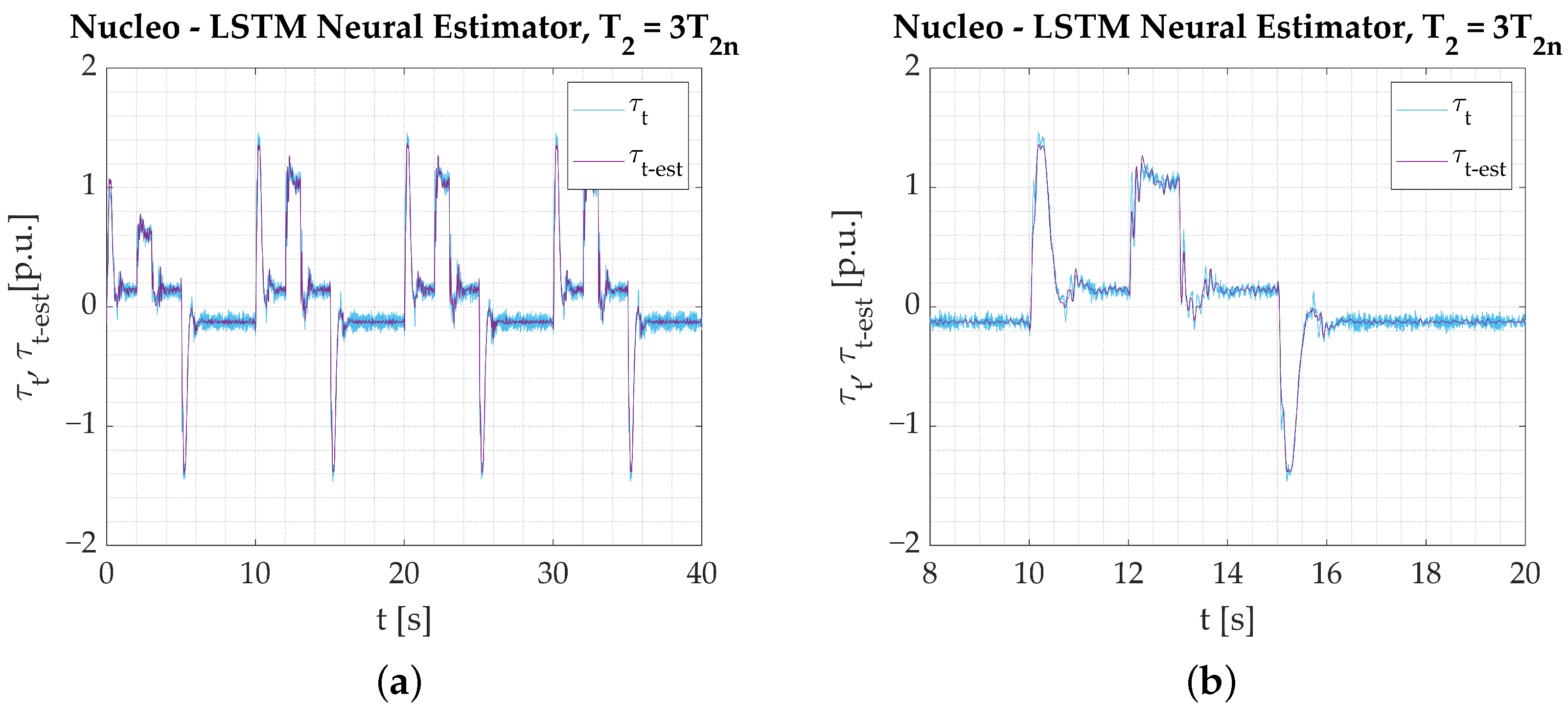
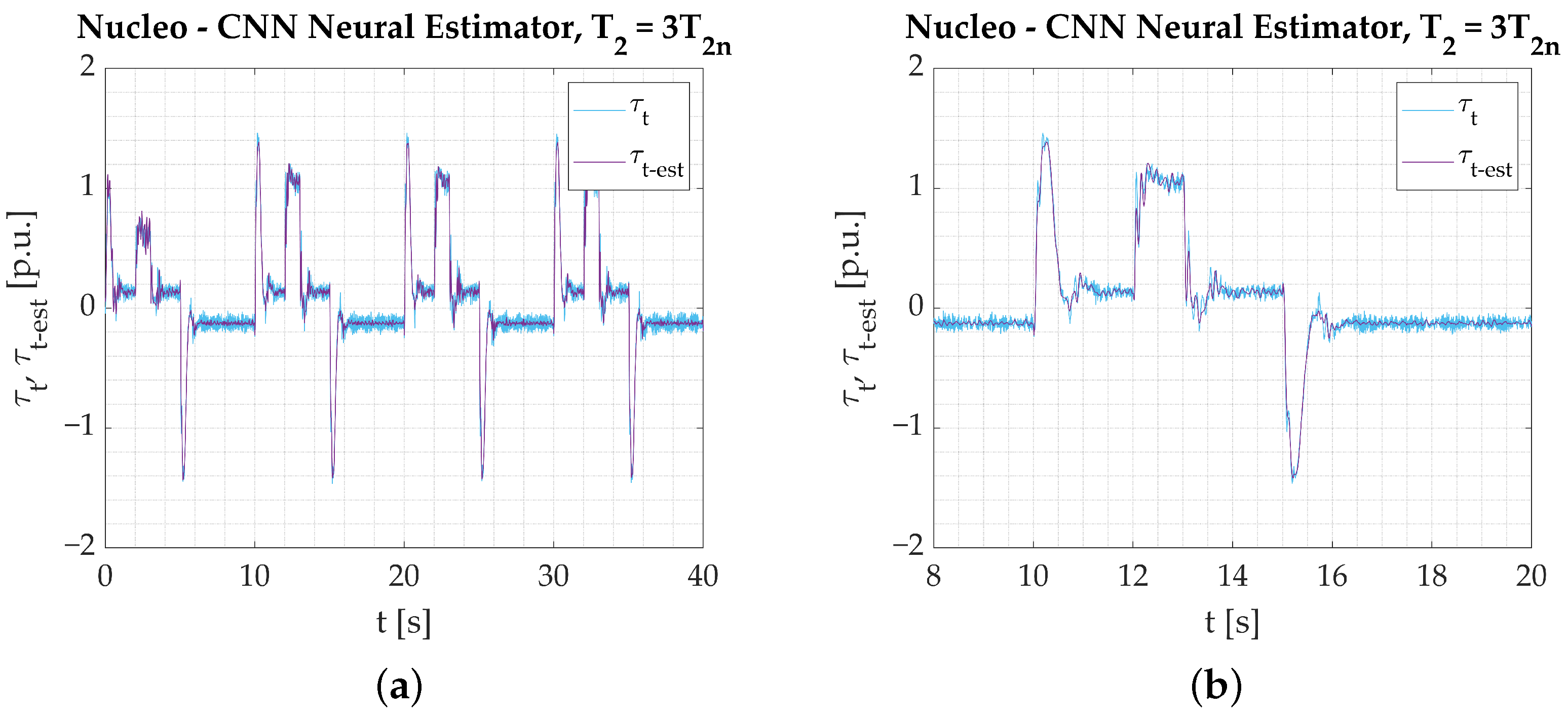
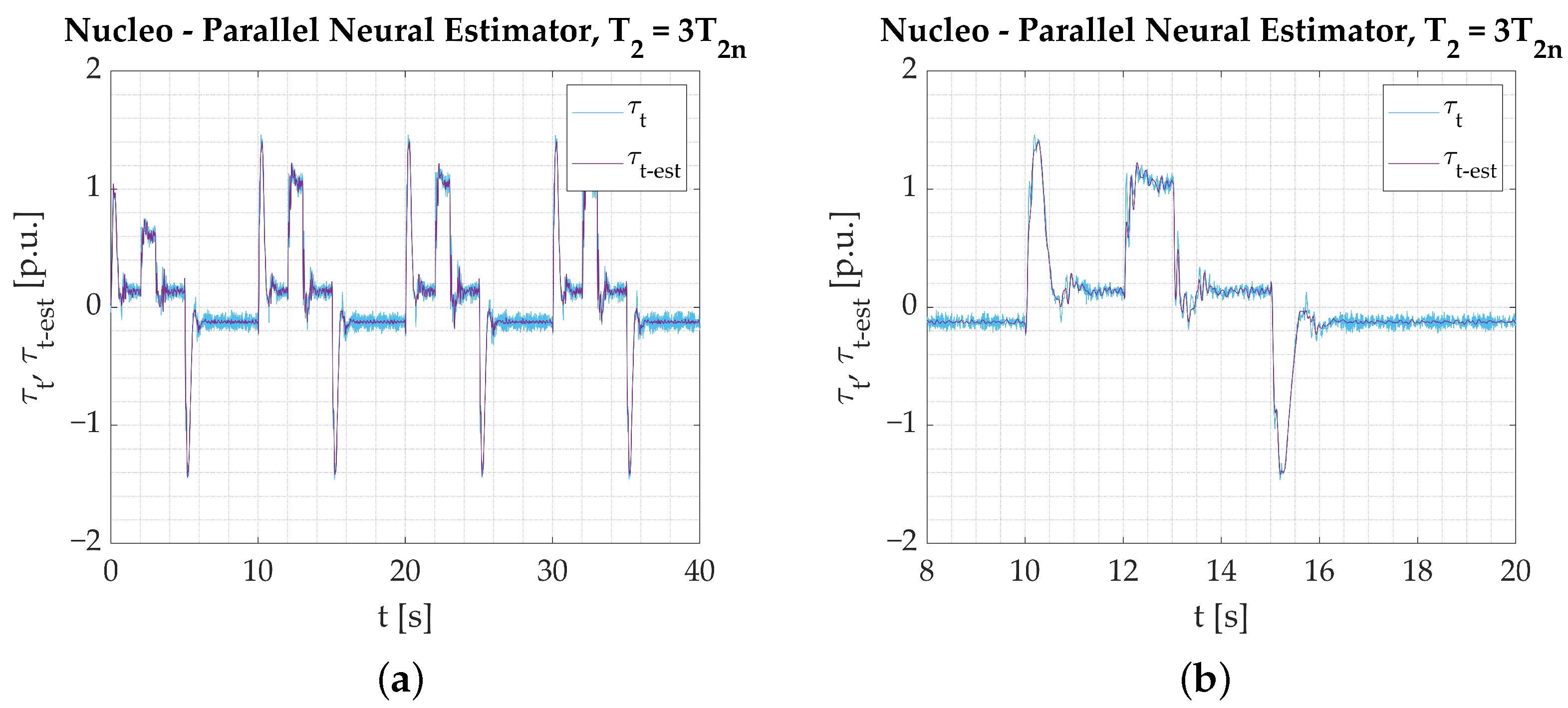
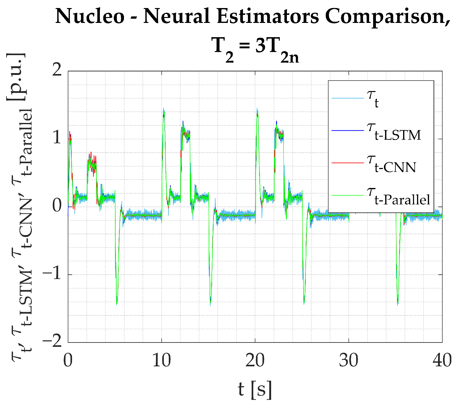
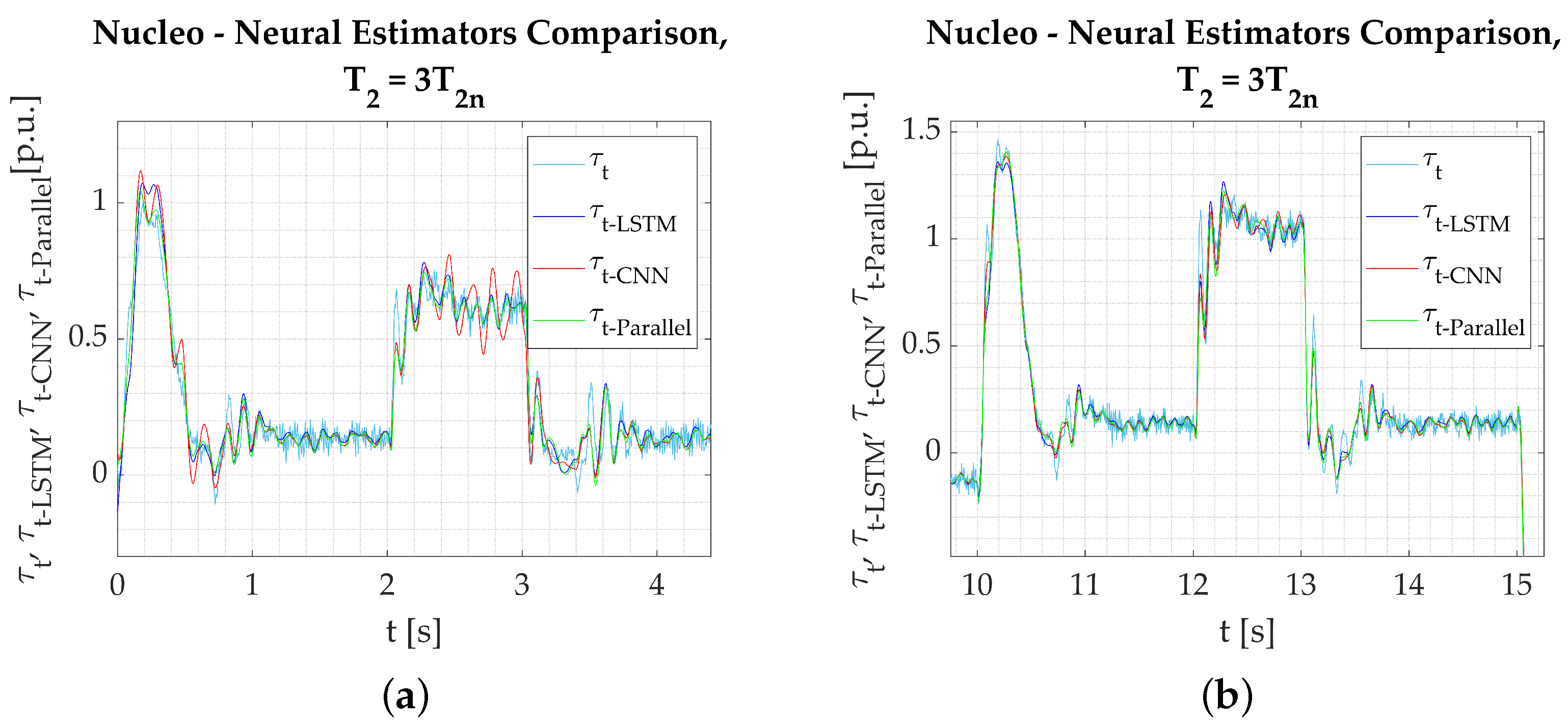
• The calculations performed on the experimental data obtained from the test bench confirm the assumptions from simulation studies. All the networks provide a good reaction to dynamic states and show their applicability to real-time verification. Among the three tested models, the Parallel Neural Network provides the most accurate coverage of all dynamic states (rapid change in direction, reaction to load torque). The worst-performing network for the nominal plant parameters is the LSTM. The output signal is not well amplified during reversions. There is an error in the steady state when load torque is activated, and the peaks are not projected well when the signal is in negative values. CNN results are better; however, it is also unable to precisely estimate the torsional torque when the load is applied.
• Establishing a performance factor may not serve as a basis for fair comparison in this study because convolution affects the network output in the steady states. The applied filtering adds to the estimation error, but it is not necessarily a negative outcome that needs to be penalized. That is why it is preferred that the performance of the networks is assessed solely on the graphical interpretation of the obtained results.
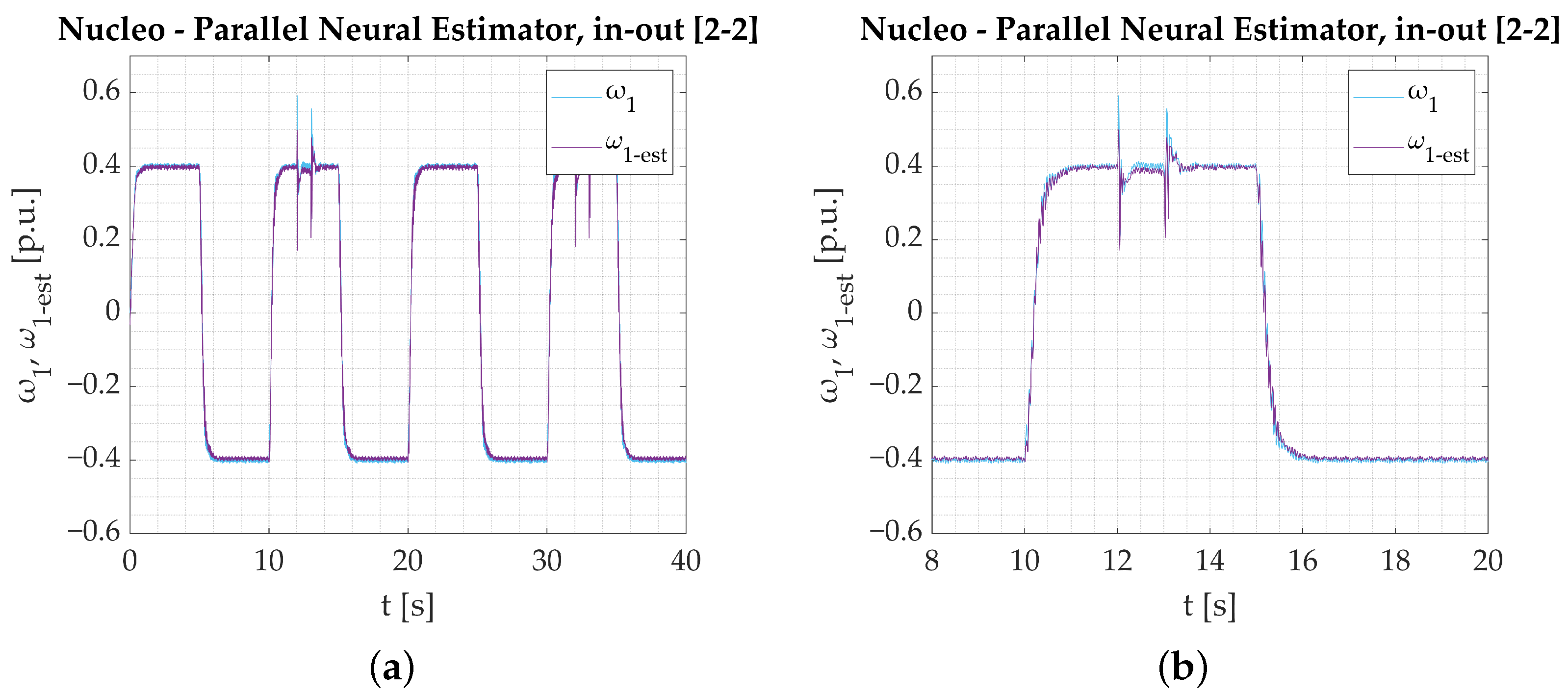
• The Parallel Neural Network enables the estimation of more than one state variable without significant structure modification. Only the output vector must be extended. To obtain comparable results, longer and more precise training needs to be conducted. It is believed that the estimation error could be related to the number of estimated signals. This could be verified in future research.
• Extending the input vector with additional signals greatly improves the performance of shallow networks. In the presented research, however, the proposed deep parallel neural model was not positively affected by such an addition. Only additional noise was inserted into the output. No beneficial effects are observed in this case. It is speculated that further training might bring positive results, but the results shown in the article do not endorse the need for further research in this direction.
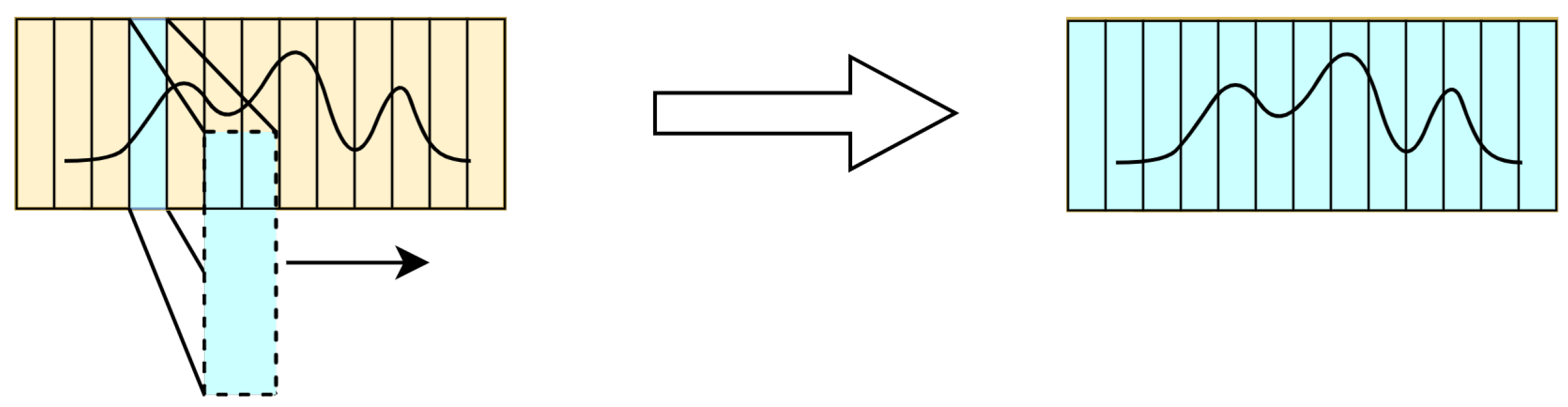
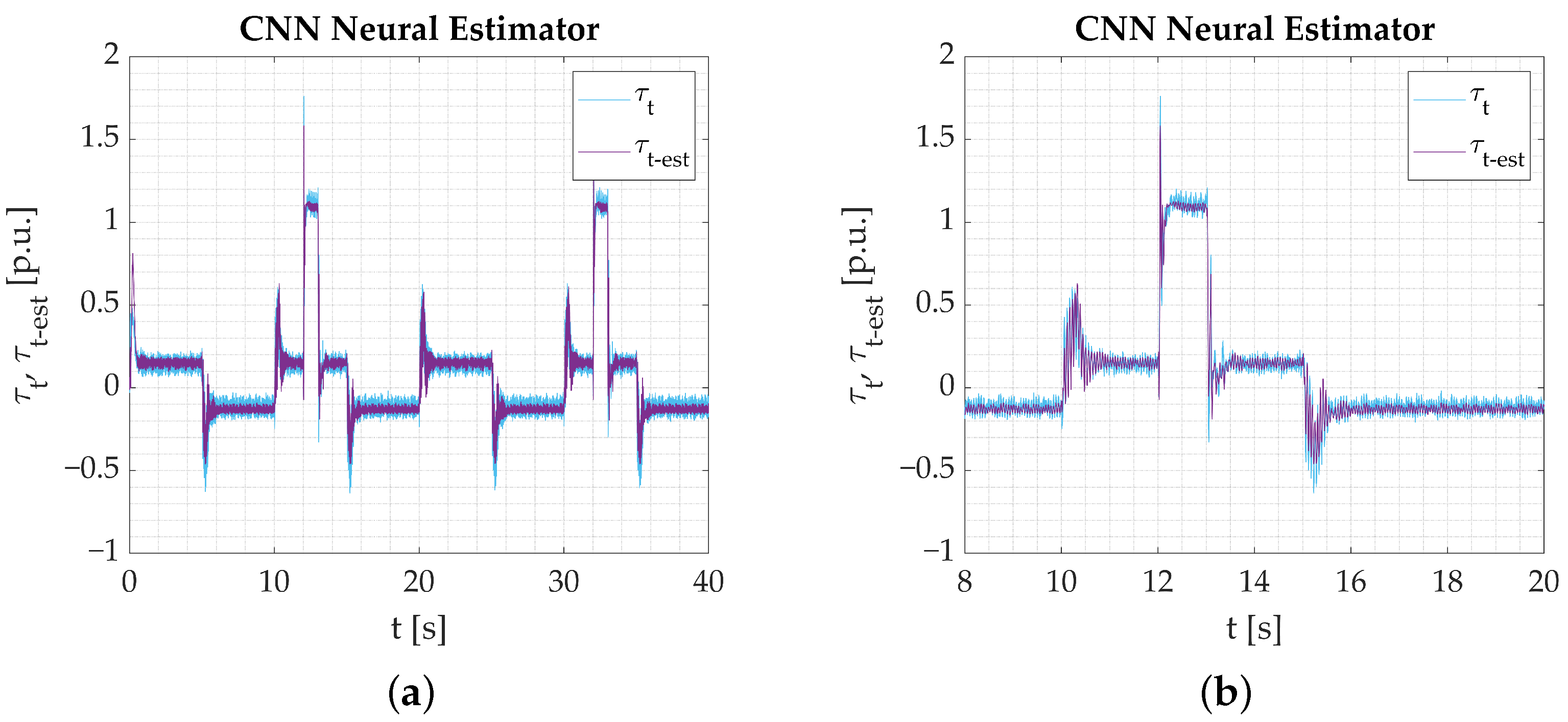
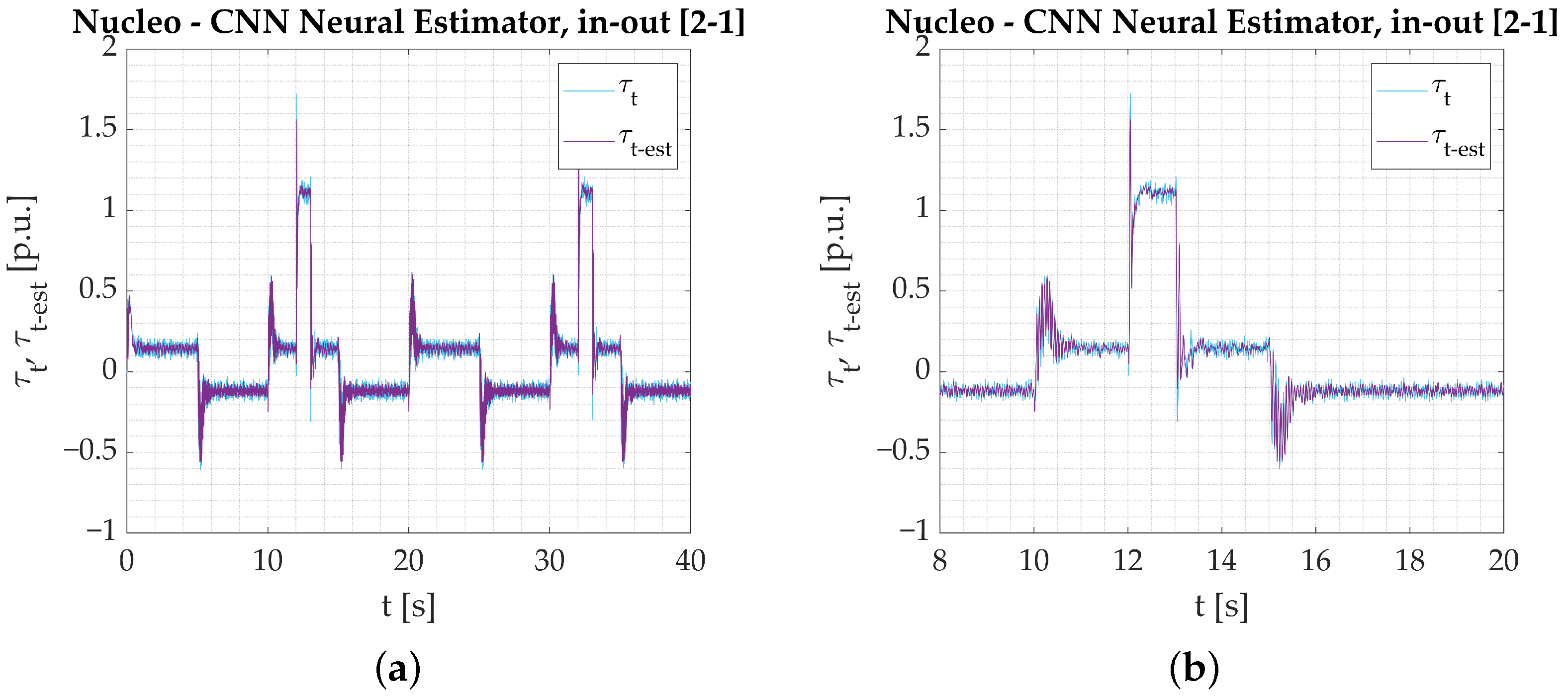
• Deep neural models prepared to operate in the ARM processor were trained on a dedicated dataset. The original data needed to be downsampled to adhere to the device calculation capabilities. Thanks to that, the training time was also reduced, the networks became more robust against measurement noise (better data generalization), and the characteristic features were easier to distinguish, which helped balance the gathered dataset and improve model performance.
• The ARM neural network execution results in visually similar outcomes. That is the reason the estimation error is used to objectively compare the acquired estimator outputs. It proves that estimated torsional torque data sets differ negligibly.
• The use of deep-learning techniques allows the accomplishment of multivariable estimation tasks without having to modify the neural network structure. Even though in this work, estimation of motor speed was performed, similar steps could be taken to obtain the estimation of the load machine speed ${\omega }_2$.
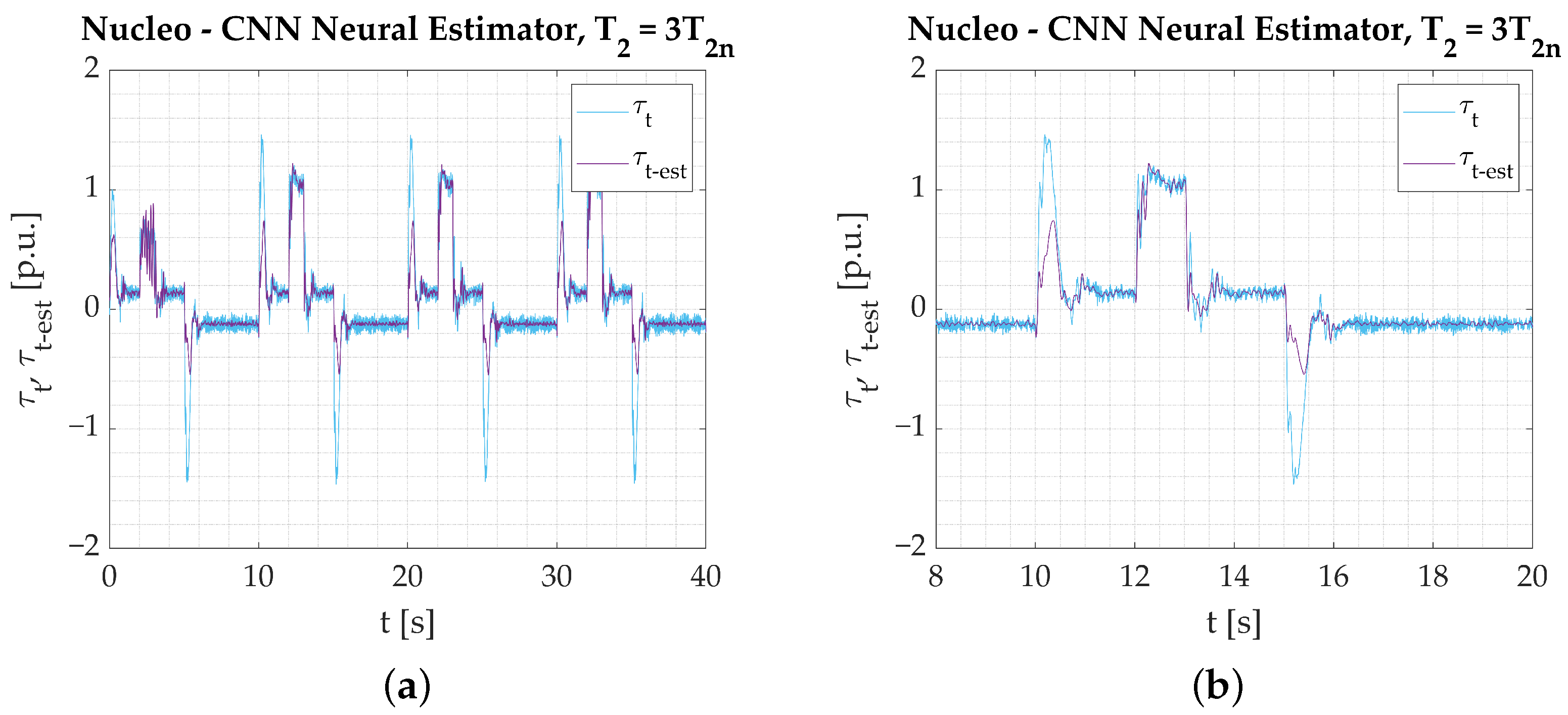
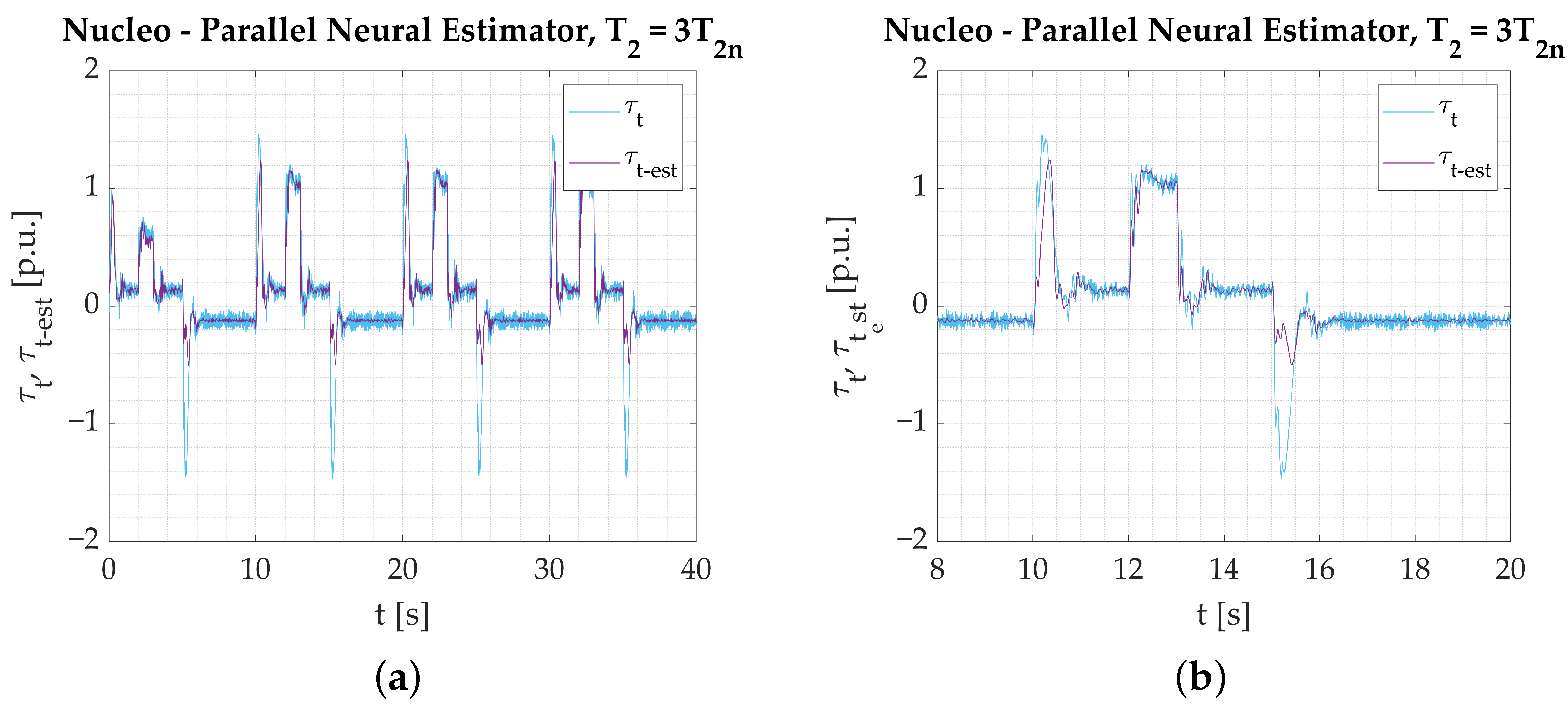
• Changing the plant parameters in the next part of experimental tests clearly emphasizes the differences between tested structures (in case those changes are not included in the training process).
• Applied modification of the training dataset involves one speed return inclusion (for the changed plant parameters) only. That leads to the conclusion that even a gentle modification of the training dataset may remarkably extend a variety of circumstances for which a network is prepared. It may also prepare the neural structure to work at different operational points without the necessity of adjusting the estimator parameters after being deployed.
• The differences noticed between particular network responses are negligible. Thus, the estimation error is calculated again. After conducting the final estimation error analysis, it turns out that (Table 5) the Parallel [2-1] neural estimator features the best response.
• It is worth noting that conducting the estimation error analytically does not always provide an objective, unambiguous review. The estimation error value obtained for the CNN Neural Network (with plant parameters change included in the training process) differs from the one calculated for the Parallel [2-1] network marginally. However, transients of the predicted variables (during the early stage of the drive work, Figure 39a—t = 2–3 s) accentuate unwanted fluctuations, which may be dangerous in real-life scenarios. It would raise a serious concern if the estimated torsional torque variable were part of a closed-loop control system.
• To conclude all research results objectively, the obtained $E_r$ increase factors are compared with the results acquired for nominal plant parameters. Final factor values are calculated according to the same criteria. The final estimation error increase comparison is applied for real-time network execution only, as the presented approach (in the authors’ opinion) constitutes the most vulnerable case, which is also mandatory from the real-life application point of view.
• The smallest increase of the estimation error for significant change in the plant parameters (not included in the training data) is noticed in the case of the Parallel [2-1] neural estimator. It leads to the conclusion that the Parallel Neural Network features the highest robustness to unpredictable circumstances that may occur in real-life scenarios.
• The proposed deep neural estimators have been proven to feature satisfying responses combined with high robustness to the changed plant parameters and the capability of being prepared for different operational points at once. However, the issue of practical, industrial deployment often forces the need for conducting additional adjustments of existing machines/factory lines. The complexity of modern industry involves a variety of different communication protocols, analog and digital sensors, resolution of the transferred data or different sample time steps. Thus, it turns out that the hypothetical implementation of the new solution may often lead to different difficulties, which may dishearten engineers and workers. The choice of an STM-based platform not only provides the versatility of the established tool but also makes the whole implementation process feasible. The Cortex M7 offers a variety of different communication protocols (including CAN bus), a wide range of different clock frequencies it can work with, and a broad range of different internal peripherals. All the mentioned advantages make the Nucleo a perfect base, which makes the deployment process easy and affordable.

References

1. Li, W.; Xue, J.; Fan, X.; Zhu, L. Loss Analysis of Permanent Magnet Synchronous Motor System Based on Strategy-Circuit-Field Co-Simulation and an Accurate Iron Loss Calculation Method. IEEE Access 2024, 12, 168339–168348. [Google Scholar] [CrossRef]
2. Wang, X.; Shen, J.; Sun, S.; Xiao, D.; Liu, Y.; Wang, Z. General Modeling and Control of Multiple Three-Phase PMSM Drives. IEEE Trans. Power Electron. 2025, 40, 1900–1909. [Google Scholar] [CrossRef]
3. Giesbrecht, M.; Torllone de Carvalho Ferreira, G.; Raimundo da Silva, R.; Milfont, L.D. Electric Machine Design and Fault Diagnosis for Electric Aircraft Propulsion in the Context of the Engineering Research Center for the Aerial Mobility of the Future. In Proceedings of the 2023 IEEE Workshop on Power Electronics for Aerospace Applications (PEASA), Nottingham, UK, 18–19 July 2023; pp. 1–5. [Google Scholar] [CrossRef]
4. Rivas-Martínez, G.I.; Rodas, J.; Herrera, E.; Doval-Gandoy, J. A Novel Approach to Performance Evaluation of Current Controllers in Power Converters and Electric Drives Using Non-Parametric Analysis. IEEE Lat. Am. Trans. 2025, 23, 68–77. [Google Scholar] [CrossRef]
5. Orlowska-Kowalska, T.; Wolkiewicz, M.; Pietrzak, P.; Skowron, M.; Ewert, P.; Tarchala, G.; Krzysztofiak, M.; Kowalski, C.T. Fault Diagnosis and Fault-Tolerant Control of PMSM Drives—State of the Art and Future Challenges. IEEE Access 2022, 10, 59979–60024. [Google Scholar] [CrossRef]
6. Pajchrowski, T.; Siwek, P.; Wójcik, A. Adaptive Neural Controller for Speed Control of PMSM with Torque Ripples. In Proceedings of the 2022 IEEE 20th International Power Electronics and Motion Control Conference (PEMC), Brasov, Romania, 25–28 September 2022; pp. 564–570. [Google Scholar] [CrossRef]
7. Niewiara, L.J.; Tarczewski, T.; Gierczynski, M.; Grzesiak, L.M. Designing a Hybrid State Feedback Control Structure for a Drive With a Reluctance Synchronous Motor. IEEE Trans. Ind. Electron. 2024, 71, 8351–8361. [Google Scholar] [CrossRef]
8. Kaminski, M.; Tarczewski, T. Neural Network Applications in Electrical Drives—Trends in Control, Estimation, Diagnostics, and Construction. Energies 2023, 16, 4441. [Google Scholar] [CrossRef]
9. Wang, F.; Wei, Y.; Young, H.; Ke, D.; Yu, X.; Rodríguez, J. Low-Stagnation Model-Free Predictive Current Control of PMSM Drives. IEEE Trans. Ind. Electron. 2024, 1–12. [Google Scholar] [CrossRef]
10. Wang, Y.; Li, P.; Shen, J.X.; Jiang, C.; Huang, X.; Long, T. Adaptive Periodic Disturbance Observer Based on Fuzzy Logic Compensation for Speed Fluctuation Suppression of PMSM Under Periodic Loads. IEEE Trans. Ind. Appl. 2024, 60, 5751–5762. [Google Scholar] [CrossRef]
11. Miyahara, K.; Katsura, S. Energy Localization in Spring-Motor Coupling System by Switching Mass Control. In Proceedings of the 2023 IEEE International Conference on Mechatronics (ICM), Loughborough, UK, 15–17 March 2023; pp. 1–6. [Google Scholar] [CrossRef]
12. Takeuchi, I.; Kaneda, T.; Katsura, S. Modeling and Control of Two-mass Resonant System Based on Element Description Method. In Proceedings of the 2021 IEEE 30th International Symposium on Industrial Electronics (ISIE), Kyoto, Japan, 20–23 June 2021; pp. 1–6. [Google Scholar] [CrossRef]
13. Szabat, K.; Orlowska-Kowalska, T. Vibration Suppression in a Two-Mass Drive System Using PI Speed Controller and Additional Feedbacks—Comparative Study. IEEE Trans. Ind. Electron. 2007, 54, 1193–1206. [Google Scholar] [CrossRef]
14. Wang, C.; Yang, M.; Zheng, W.; Long, J.; Xu, D. Vibration Suppression With Shaft Torque Limitation Using Explicit MPC-PI Switching Control in Elastic Drive Systems. IEEE Trans. Ind. Electron. 2015, 62, 6855–6867. [Google Scholar] [CrossRef]
15. Brock, S.; Łuczak, D.; Nowopolski, K.; Pajchrowski, T.; Zawirski, K. Two Approaches to Speed Control for Multi-Mass System With Variable Mechanical Parameters. IEEE Trans. Ind. Electron. 2017, 64, 3338–3347. [Google Scholar] [CrossRef]
16. Zoubek, H.; Pacas, M. Encoderless Identification of Two-Mass-Systems Utilizing an Extended Speed Adaptive Observer Structure. IEEE Trans. Ind. Electron. 2017, 64, 595–604. [Google Scholar] [CrossRef]
17. Yang, Q.; Mao, K.; Zheng, S.; Le, Y. Rotor Position Estimation Based on Fast Terminal Sliding Mode for Magnetic Suspension Centrifugal Compressor Drives. IEEE Trans. Instrum. Meas. 2024, 73, 1–11. [Google Scholar] [CrossRef]
18. Wang, T.; Yu, Y.; Zhang, Z.; Jin, S.; Wang, B.; Xu, D. An Auxiliary Variable-Based MRAS Speed Observer for Stable Wide-Speed Operation in Sensorless Induction Motor Drives. IEEE J. Emerg. Sel. Top. Power Electron. 2024, 12, 4926–4940. [Google Scholar] [CrossRef]
19. Liu, Y.; Li, H.; He, W. Rotor Position Estimation Method for Permanent Magnet Synchronous Motor Based on High-Order Extended Kalman Filter. Electronics 2024, 13, 4978. [Google Scholar] [CrossRef]
20. Liu, J.; Li, M.; Xie, E. Noncascade Structure Equivalent SMC for PMSM Driving Based on Improved ESO. IEEE Trans. Power Electron. 2025, 40, 611–624. [Google Scholar] [CrossRef]
21. Li, H.; Zhang, R.; Shi, P.; Xiao, P.; Zheng, K.; Qiu, T. State Parameters Estimation for Distributed Drive Electric Vehicle Based on PMSMs’ Sensorless Control. IEEE Sens. J. 2024, 24, 24054–24069. [Google Scholar] [CrossRef]
22. Djellouli, Y.; El Mehdi ARDJOUN, S.A.; Zerdali, E.; Denai, M.; Chafouk, H. Real Time Implementation of a Speed/Torque Sensorless Observer for Induction Motor Utilizing Extended Kalman Filtering Technique. In Proceedings of the 2024 3rd International Conference on Advanced Electrical Engineering (ICAEE), Sidi-Bel-Abbes, Algeria, 5–7 November 2024; pp. 1–5. [Google Scholar] [CrossRef]
23. Chen, Z.; Chen, F.; Huang, X.; Li, Z.; Wu, M. DEA-tuning of Reduced-order Extended Luenberger Sliding Mode Observers(ELSMO) for Sensorless Control of High-speed SPMSM. In Proceedings of the 2021 IEEE International Electric Machines & Drives Conference (IEMDC), Hartford, CT, USA, 17–20 May 2021; pp. 1–7. [Google Scholar] [CrossRef]
24. Reddy, S.V.B.S.; Kumar, B.; Swaroop, D. Investigations on Training Algorithms for Neural Networks Based Flux Estimator Used in Speed Estimation of Induction Motor. In Proceedings of the 2019 6th International Conference on Signal Processing and Integrated Networks (SPIN), Noida, India, 7–8 March 2019; pp. 1090–1094. [Google Scholar] [CrossRef]
25. Zhang, X.; Jiang, Q. Research on Sensorless Control of PMSM Based on Fuzzy Sliding Mode Observer. In Proceedings of the 2021 IEEE 16th Conference on Industrial Electronics and Applications (ICIEA), Chengdu, China, 1–4 August 2021; pp. 213–218. [Google Scholar] [CrossRef]
26. Lin, X.; Xu, R.; Yao, W.; Gao, Y.; Sun, G.; Liu, J.; Peretti, L.; Wu, L. Observer-Based Prescribed Performance Speed Control for PMSMs: A Data-Driven RBF Neural Network Approach. IEEE Trans. Ind. Inform. 2024, 20, 7502–7512. [Google Scholar] [CrossRef]
27. Soufyane, B.; Abdelhamid, R.; Smail, Z. Signed-Distance Fuzzy Logic Controller Adaptation Mechanism based MRAS Observer for Direct-Drive PMSG Wind Turbines Sensorless Control. In Proceedings of the 2020 American Control Conference (ACC), Denver, CO, USA, 1–3 July 2020; pp. 4083–4089. [Google Scholar] [CrossRef]
28. Erenturk, K. Gray-fuzzy control of a nonlinear two-mass system. J. Frankl. Inst. 2010, 347, 1171–1185. [Google Scholar] [CrossRef]
29. Deponti, M.; Pejovski, D.; Gerlando, A.D.; Perini, R. A Nonlinear Extended State Observer Design for Torsional Vibrations Estimation in PMSM Drive. In Proceedings of the 2024 International Conference on Electrical Machines (ICEM), Torino, Italy, 1–4 September 2024; pp. 1–7. [Google Scholar] [CrossRef]
30. Kaminski, M. Adaptive Gradient-Based Luenberger Observer Implemented for Electric Drive with Elastic Joint. In Proceedings of the 2018 23rd International Conference on Methods & Models in Automation & Robotics (MMAR), Miedzyzdroje, Poland, 27–30 August 2018; pp. 53–58. [Google Scholar] [CrossRef]
31. Liu, Y.; Song, B.; Zhou, X.; Gao, Y.; Chen, T. An Adaptive Torque Observer Based on Fuzzy Inference for Flexible Joint Application. Machines 2023, 11, 794. [Google Scholar] [CrossRef]
32. Szabat, K.; Tran-Van, T.; Kaminski, M. A Modified Fuzzy Luenberger Observer for a Two-Mass Drive System. IEEE Trans. Ind. Inform. 2015, 11, 531–539. [Google Scholar] [CrossRef]
33. Auger, F.; Hilairet, M.; Guerrero, J.M.; Monmasson, E.; Orlowska-Kowalska, T.; Katsura, S. Industrial Applications of the Kalman Filter: A Review. IEEE Trans. Ind. Electron. 2013, 60, 5458–5471. [Google Scholar] [CrossRef]
34. Szabat, K.; Orlowska-Kowalska, T. Application of the Kalman Filters to the High-Performance Drive System With Elastic Coupling. IEEE Trans. Ind. Electron. 2012, 59, 4226–4235. [Google Scholar] [CrossRef]
35. Szabat, K.; Orlowska-Kowalska, T. Performance Improvement of Industrial Drives With Mechanical Elasticity Using Nonlinear Adaptive Kalman Filter. IEEE Trans. Ind. Electron. 2008, 55, 1075–1084. [Google Scholar] [CrossRef]
36. Szabat, K.; Wróbel, K.; Dróżdż, K.; Janiszewski, D.; Pajchrowski, T.; Wójcik, A. A Fuzzy Unscented Kalman Filter in the Adaptive Control System of a Drive System with a Flexible Joint. Energies 2020, 13, 2056. [Google Scholar] [CrossRef]
37. Szabat, K.; Wróbel, K.; Śleszycki, K.; Katsura, S. States Estimation of the Two-Mass Drive System Using Multilayer Observer. In Proceedings of the 2021 IEEE 19th International Power Electronics and Motion Control Conference (PEMC), Gliwice, Poland, 25–29 April 2021; pp. 743–748. [Google Scholar] [CrossRef]
38. Szabat, K.; Tokarczyk, A.; Wróbel, K.; Katsura, S. Application of the Multi-Layer Observer for a Two-Mass Drive System. In Proceedings of the 2020 IEEE 29th International Symposium on Industrial Electronics (ISIE), Delft, The Netherlands, 17–19 June 2020; pp. 265–270. [Google Scholar] [CrossRef]
39. Abiodun, O.I.; Jantan, A.; Omolara, A.E.; Dada, K.V.; Mohamed, N.A.; Arshad, H. State-of-the-art in artificial neural network applications: A survey. Heliyon 2018, 4, e00938. [Google Scholar] [CrossRef]
40. Widrow, B.; Lehr, M. 30 years of adaptive neural networks: Perceptron, Madaline, and backpropagation. Proc. IEEE 1990, 78, 1415–1442. [Google Scholar] [CrossRef]
41. Orlowska-Kowalska, T.; Szabat, K. Neural-Network Application for Mechanical Variables Estimation of a Two-Mass Drive System. IEEE Trans. Ind. Electron. 2007, 54, 1352–1364. [Google Scholar] [CrossRef]
42. Belov, M.P.; Van Lanh, N.; Khoa, T.D. State Observer based Elman Recurrent Neural Network for Electric Drive of Optical-Mechanical Complexes. In Proceedings of the 2021 IEEE Conference of Russian Young Researchers in Electrical and Electronic Engineering (ElConRus), St. Petersburg, Moscow, Russia, 26–29 January 2021; pp. 802–805. [Google Scholar] [CrossRef]
43. Nicola, M.; Nicola, C.I.; Duţă, M. Sensorless Control of PMSM using FOC Strategy Based on Multiple ANN and Load Torque Observer. In Proceedings of the 2020 International Conference on Development and Application Systems (DAS), Suceava, Romania, 21–23 May 2020; pp. 32–37. [Google Scholar] [CrossRef]
44. Zhang, S.; Wallscheid, O.; Porrmann, M. Machine Learning for the Control and Monitoring of Electric Machine Drives: Advances and Trends. IEEE Open J. Ind. Appl. 2023, 4, 188–214. [Google Scholar] [CrossRef]
45. Orlowska-Kowalska, T.; Kaminski, M. Effectiveness of Saliency-Based Methods in Optimization of Neural State Estimators of the Drive System With Elastic Couplings. IEEE Trans. Ind. Electron. 2009, 56, 4043–4051. [Google Scholar] [CrossRef]
46. Łuczak, D.; Wójcik, A. The study of neural estimator structure influence on the estimation quality of selected state variables of the complex mechanical part of electrical drive. In Proceedings of the 2017 19th European Conference on Power Electronics and Applications (EPE’17 ECCE Europe), Warsaw, Poland, 11–14 September 2017; pp. P.1–P.10. [Google Scholar] [CrossRef]
47. Orlowska-Kowalska, T.; Kaminski, M. FPGA Implementation of the Multilayer Neural Network for the Speed Estimation of the Two-Mass Drive System. IEEE Trans. Ind. Inform. 2011, 7, 436–445. [Google Scholar] [CrossRef]
48. Mathesh, G.; Saravanakumar, R.; Salgotra, R. Novel Machine Learning Control for Power Management Using an Instantaneous Reference Current in Multiple-Source-Fed Electric Vehicles. Energies 2024, 17, 2677. [Google Scholar] [CrossRef]
49. Lin, F.J.; Huang, M.S.; Chen, S.G.; Hsu, C.W.; Liang, C.H. Adaptive Backstepping Control for Synchronous Reluctance Motor Based on Intelligent Current Angle Control. IEEE Trans. Power Electron. 2020, 35, 7465–7479. [Google Scholar] [CrossRef]
50. Malarczyk, M.; Zychlewicz, M.; Stanislawski, R.; Kaminski, M. Electric Drive with an Adaptive Controller and Wireless Communication System. Future Internet 2023, 15, 49. [Google Scholar] [CrossRef]
51. Liu, W.; Wang, Z.; Liu, X.; Zeng, N.; Liu, Y.; Alsaadi, F.E. A survey of deep neural network architectures and their applications. Neurocomputing 2017, 234, 11–26. [Google Scholar] [CrossRef]
52. Li, Z.; Liu, F.; Yang, W.; Peng, S.; Zhou, J. A Survey of Convolutional Neural Networks: Analysis, Applications, and Prospects. IEEE Trans. Neural Netw. Learn. Syst. 2022, 33, 6999–7019. [Google Scholar] [CrossRef]
53. Mustafa, A.; Sasamura, T.; Morita, T. Sensorless Speed Control of Ultrasonic Motors Using Deep Reinforcement Learning. IEEE Sens. J. 2024, 24, 4023–4035. [Google Scholar] [CrossRef]
54. Li, Y.; Sun, T.; Zhang, W.; Li, S.; Liang, J.; Wang, Z. A Torque Observer for IPMSM Drives Based on Deep Neural Network. In Proceedings of the 2019 14th IEEE Conference on Industrial Electronics and Applications (ICIEA), Xi’an, China, 19–21 June 2019; pp. 1530–1535. [Google Scholar] [CrossRef]
55. Derugo, P.; Kahsay, A.H.; Szabat, K.; Shikata, K.; Katsura, S. A Novel PI-Based Control Structure with Additional Feedback from Torsional Torque and Its Derivative for Damping Torsional Vibrations. Energies 2024, 17, 4786. [Google Scholar] [CrossRef]
56. Ogata, K. Modern Control Engineering; Prentice Hall: Hoboken, NJ, USA, 2002. [Google Scholar]
57. Åström, K.; Murray, R. Feedback Systems: An Introduction for Scientists and Engineers, Second Edition; Princeton University Press: Princeton, NJ, USA, 2021. [Google Scholar]
58. Ackermann, J. Der Entwurf linearer Regelungssysteme im Zustandsraum. Automatisierungstechnik 1972, 20, 297–300. [Google Scholar] [CrossRef]
59. Frobenius, G. Ueber lineare Substitutionen und bilineare Formen. J. Reine Angew. Math. 1877, 84, 1–63. [Google Scholar]
Figure 1. Two-mass system control using a state feedback controller with integral action.
Energies 18 00568 g001
Figure 2. The idea of one-dimensional convolution operation.
Energies 18 00568 g002
Figure 3. The idea of one-dimensional maxpooling operation.
Energies 18 00568 g003
Figure 4. The internal structure of the long short-term memory unit.
Energies 18 00568 g004
Figure 5. The general architecture of the LSTM Neural Network described in the paper.
Energies 18 00568 g005
Figure 6. The general topology of the CNN Neural Network described in the paper.
Energies 18 00568 g006
Figure 7. The first part (Preliminary Data Processing) of the Parallel Neural Network proposed in the paper.
Energies 18 00568 g007
Figure 8. The second part (Fully Connected Layers) of the Parallel Neural Network proposed in the paper.
Energies 18 00568 g008
Figure 9. The internal structure of the proposed LSTM Neural Network created in Matlab—Deep Network Designer tool.
Energies 18 00568 g009
Figure 10. The internal structure of the proposed CNN Neural Network created in Matlab—Deep Network Designer tool.
Energies 18 00568 g010
Figure 11. The internal structure of the proposed Parallel Neural Network created in Matlab—Deep Network Designer tool.
Energies 18 00568 g011
Figure 12. Transient of the neural network validation dataset–input vector.
Energies 18 00568 g012
Figure 13. Transient of obtained results for the LSTM Neural Network: (a) response to training data, (b) response to the reference trajectory shown in Figure 12.
Energies 18 00568 g013
Figure 14. Transient of obtained results for the CNN Neural Network: (a) response to training data, (b) response to the reference trajectory shown in Figure 12.
Energies 18 00568 g014
Figure 15. Transient of obtained results for the Parallel Neural Network: (a) response to training data, (b) response to the reference trajectory shown in Figure 12.
Energies 18 00568 g015
Figure 16. Transient of particular signals used in additional test: (a) reference speed and load torque trajectory, (b) LSTM estimator response for the reference trajectories shown in (a).
Energies 18 00568 g016
Figure 17. Transients of obtained results during the additional test for the reference trajectories shown in Figure 16a: (a) CNN estimator response, (b) Parallel estimator response.
Energies 18 00568 g017
Figure 18. Schematic of the laboratory equipment connections.
Energies 18 00568 g018
Figure 19. Picture of the laboratory test bench.
Energies 18 00568 g019
Figure 20. Estimated torsional torque transients obtained for the LSTM Neural Network: (a) the overall transient review, (b) a zoom-in showing dynamic states of the drive and additional load torque attachment moment.
Energies 18 00568 g020
Figure 21. Estimated Torsional Torque transients obtained for the CNN Neural Network: (a) the overall transient review, (b) a zoom-in showing dynamic states of the drive and additional load torque attachment moment.
Energies 18 00568 g021
Figure 22. Estimated Torsional Torque transients obtained for the Parallel [2-1] Neural Network: (a) the overall transient review, (b) a zoom-in showing dynamics states of the drive and additional load torque attachment moment.
Energies 18 00568 g022
Figure 23. Estimated Speed transients obtained for the Parallel [2-2] Neural Network: (a) the overall transient review, (b) a zoom-in showing dynamics states of the drive and additional load torque attachment moment.
Energies 18 00568 g023
Figure 24. Estimated Torsional Torque transients obtained for the Parallel [2-2] Neural Network: (a) the overall transient review, (b) a zoom-in showing dynamics states of the drive and additional load torque attachment moment.
Energies 18 00568 g024
Figure 25. Estimated Speed transients obtained for the Parallel [6-2] Neural Network: (a) the overall transient review, (b) a zoom-in showing dynamics states of the drive and additional load torque attachment moment.
Energies 18 00568 g025
Figure 26. Estimated Torsional Torque transients obtained for the Parallel [6-2] Neural Network: (a) the overall transient review, (b) a zoom-in showing dynamics states of the drive and additional load torque attachment moment.
Energies 18 00568 g026
Figure 27. Estimated Torsional Torque transients obtained for the LSTM Neural Network during real-time execution: (a) the overall transient review, (b) a zoom-in showing dynamics states of the drive and additional load torque attachment moment.
Energies 18 00568 g027
Figure 28. Estimated Torsional Torque transients obtained for the CNN Neural Network during real-time execution: (a) the overall transient review, (b) a zoom-in showing dynamics states of the drive and additional load torque attachment moment.
Energies 18 00568 g028
Figure 29. Estimated Torsional Torque transients obtained for the Parallel [2-1] Neural Network during real-time execution: (a) the overall transient review, (b) a zoom-in showing dynamics states of the drive and additional load torque attachment moment.
Energies 18 00568 g029
Figure 30. Estimated Speed transients obtained for the Parallel [2-2] Neural Network during real-time execution: (a) the overall transient review, (b) a zoom-in showing dynamics states of the drive and additional load torque attachment moment.
Energies 18 00568 g030
Figure 31. Estimated Torsional Torque transients obtained for the Parallel [2-2] Neural Network during real-time execution: (a) the overall transient review, (b) a zoom-in showing dynamics states of the drive and additional load torque attachment moment.
Energies 18 00568 g031
Figure 32. Estimated Torsional Torque transients obtained for the LSTM Neural Network and increased mechanical time constant of the load machine during real-time execution: (a) the overall transient review, (b) a zoom-in showing dynamics states of the drive and additional load torque attachment moment.
Energies 18 00568 g032
Figure 33. Estimated Torsional Torque transients obtained for the CNN Neural Network and increased mechanical time constant of the load machine during real-time execution: (a) the overall transient review, (b) a zoom-in showing dynamics states of the drive and additional load torque attachment moment.
Energies 18 00568 g033
Figure 34. Estimated Torsional Torque transients obtained for the Parallel [2-1] Neural Network and increased mechanical time constant of the load machine during real-time execution: (a) the overall transient review, (b) a zoom-in showing dynamics states of the drive and additional load torque attachment moment.
Energies 18 00568 g034
Figure 35. Estimated Torsional Torque transients obtained for the LSTM Neural Network and increased mechanical time constant (included during the training process) of the load machine during real-time execution: (a) the overall transient review, (b) a zoom-in showing dynamics states of the drive and additional load torque attachment moment.
Energies 18 00568 g035
Figure 36. Estimated Torsional Torque transients obtained for the CNN Neural Network and increased mechanical time constant (included during the training process) of the load machine during real-time execution: (a) the overall transient review, (b) a zoom-in showing dynamics states of the drive and additional load torque attachment moment.
Energies 18 00568 g036
Figure 37. Estimated Torsional Torque transients obtained for the Parallel [2-1] Neural Network and increased mechanical time constant (included during the training process) of the load machine during real-time execution: (a) the overall transient review, (b) a zoom-in showing dynamics states of the drive and additional load torque attachment moment.
Energies 18 00568 g037
Figure 38. Estimated Torsional Torque transients obtained for all three neural networks and increased mechanical time constant (included during the training process) of the load machine during real-time execution.
Energies 18 00568 g038
Figure 39. Estimated Torsional Torque transients obtained for all three neural networks and increased mechanical time constant (included during the training process) of the load machine during real-time execution: (a) a zoom-in showing the electric motor start-up, (b) a zoom-in showing dynamics states of the drive and additional load torque attachment moment.
Energies 18 00568 g039