A Novel Approach to Production Allocation for Multi-Layer Commingled Tight Gas Wells: Insights from the Ordos Basin, NW China

Abstract

During the development of multi-layer tight sandstone gas reservoirs in Ordos Basin, China, it has not been easy to calculate accurately the production of each individual layer in gas wells. However, production allocation provides a vital basis for evaluating dynamic reserves and drainage areas of gas wells and remaining gas distributions of gas layers. To improve the accuracy and reliability of production allocation of gas wells, a new model was constructed based on the seepage equation, material balance equation, and pipe string pressure equation. In particular, this new model introduced the seepage equation with an elliptical boundary to accurately capture the fluid flow characteristics within a lenticular tight gas reservoir. The new model can accurately calculate the production and reservoir pressure of each individual layer in gas wells. In addition, the new model was validated and applied in the Sulige gas field, Ordos Basin. The following conclusions were drawn: First, The gas production contribution rates of pay zones based on the new model are fairly close to the measurements of the production profile logging, with errors less than 10%. Second, The overall drainage area of a gas well lies among those of each pay zone, and the total dynamic reserves of the well are close to the sum of the dynamic reserves of pay zones. Third, Higher permeability may lead to higher initial gas production of the pay zone, but the ultimate gas production contributions of pay zones are affected jointly by permeability and dynamic reserves. Finally, The new model has been successfully applied to the SZ block of the Sulige gas field, in which the fine evaluation of dynamic reserves, drainage areas, gas production, recovery factors, and remaining gas distributions of different layers was delivered, and the application results provide technical support for the future well placement and enhanced gas recovery of the block.

1. Introduction

In the Ordos Basin, NW China, the tight sandstone reservoirs of the Upper Paleozoic Shihezi and Shanxi Formations develop multiple gas-bearing layers, and the effective sand bodies (gas layers) are characterized by the lenticular dispersed distribution, small scales, thin beds, and inferior connectivity [1,2,3,4,5,6,7]. Vertically, multiple gas layers are often perforated in a gas well to improve the well production. However, for the purpose of reducing production costs, only the production and casing pressure at the wellhead is metered for gas wells, and the production contribution of each layer cannot be accurately measured. Production allocation provides a vital basis for evaluating dynamic reserves of different layers, drainage areas, and remaining gas distributions of gas wells [8,9,10,11,12]. Numerous methods have been developed for the production allocation of gas wells, including the Formation Coefficient Method (Kh = permeability × thickness), Catastrophe Method, numerical simulation, and gas production profile logging [13,14,15,16]. Yet, they have not seen extensive applications in the industry due to their limitations. Specifically, the Formation Coefficient Method performs the weighted calculation of production contributions of different layers concerning only the Kh values, which is excessively simple and suffers from huge calculation errors [17,18]. In fact, production contributions of different layers are affected not only by permeability and pay zone thickness but also by porosity, saturation, gas layer scale, reservoir pressure, and other factors. The Catastrophe Method is a mathematical theory that is mainly used to explain abruptly changing phenomena; although it considers many factors, including reservoir physical properties, reservoir pressure, and production, it only uses mathematical theory to analyze the correlation between factors and production contribution rate, lacking a robust theoretical basis of reservoir engineering. Thus, it is still limited in its applications [19,20]. Numerical simulation has complex workflows, so it is time-consuming, and simulation results have a high dependency on accurate geological models. Production profile logging is the most accurate method among these four methods, but production profile logging is expensive, resulting in only a few gas wells that can achieve production profile logging data.

As mentioned above, these traditional models either take into account very limited factors, lack a theoretical basis for reservoir engineering or are time-consuming or expensive. In this paper, a novel model was constructed to improve the accuracy of production allocation of gas wells. Compared with traditional methods, this new model considers a wider range of parameters that influence production allocation to improve the calculation accuracy, such as the physical properties of each pay zone, geometric parameters of effective sand bodies, reservoir pressure, wellbore pressure, and gas well production. In addition, this new model has a stronger foundation of reservoir engineering because it was constructed based on a series of equations that can rationally describe the flow regime of multi-layer commingled gas wells, including seepage equation, material balance equation, pipe string pressure equation, etc. In particular, this new model introduced the seepage equation with an elliptical boundary to accurately capture the fluid flow characteristics within a lenticular tight gas reservoir. Furthermore, equations of this new model can be used to develop software, making the process of production allocation more economical and efficient. The production allocation results can be further used to improve the evaluation accuracy of dynamic reserves, drainage areas, recovery factors, and remaining gas distributions of different layers, which provide references for future good placement and enhanced recovery of gas fields.

2. Model Theory

2.1. Basic Assumptions

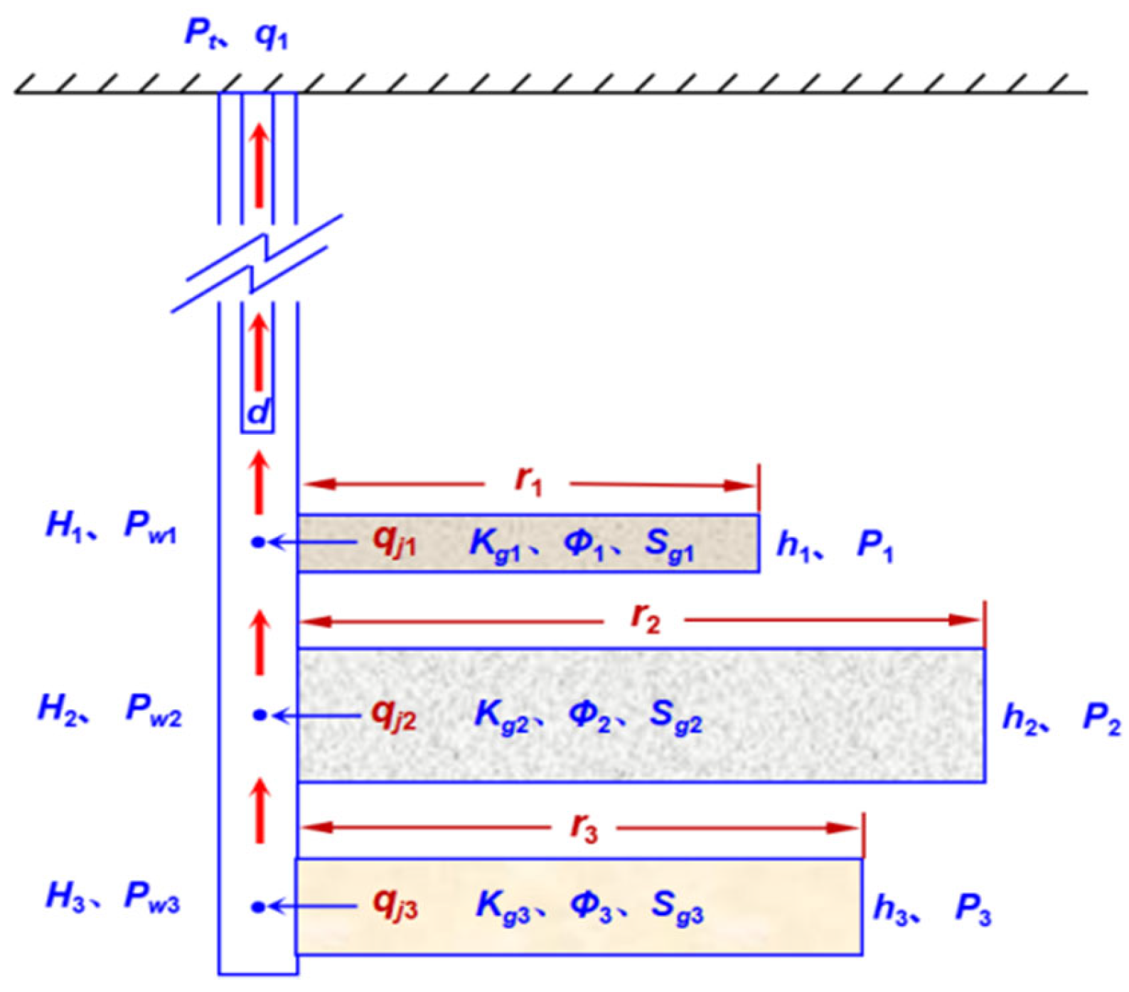
The proposed new production allocation model is shown in Figure 1. Vertically, two or more gas layers are produced simultaneously in a gas well. The model incorporates the reservoir parameters of different layers (such as lengths L, widths W, thicknesses h, porosity φ, permeability K, and gas saturations S_g of effective sand bodies), production parameters (such as reservoir pressure P, flowing bottomhole pressure P_w and production rates q) and pipe string parameters (such as tubing pressure P_t and reservoir middle depths H of different layers). The gas well production allocation is finely calculated in accordance with the coupled analysis of the reservoir, production, and pipe string parameters. To restrain the application range of the model, the following assumptions are made:

(1)

The gas reservoir is a lenticular lithological gas reservoir with no bottom and edge water. The gas reservoir presents no or weak water production.

(2)

The model is homogenous, and the reservoir physical properties of each pay zone of the gas well are isotropic.

(3)

The lenticular effective sand body is simplified into an ellipse and a gas well located in the geometric center of the ellipse. The scale of the effective sand body is moderate, with a length of <700 m and a width of <500 m. The boundary of the effective sand body is also the seepage boundary.

(4)

The well density of the well patterns in the study area is less than 4 wells/km², with no considerable well interference.

2.2. Geometric Parameters of Effective Sand Bodies

The geometric parameters of effective sand bodies of the tight sandstone gas reservoirs in the Ordos Basin were statistically analyzed via multiple approaches, such as the field outcrop observation and high-density well pattern dissection of representative blocks. The fluvial facies of the tight sandstone gas reservoirs in the Ordos Basin are mainly of the braided river and meandering river deposition. Although the fluvial channel sand bodies generally feature the style of multi-stage stacking, the effective sand bodies with favorable reservoir physical properties are mostly isolated and dispersed [21,22].

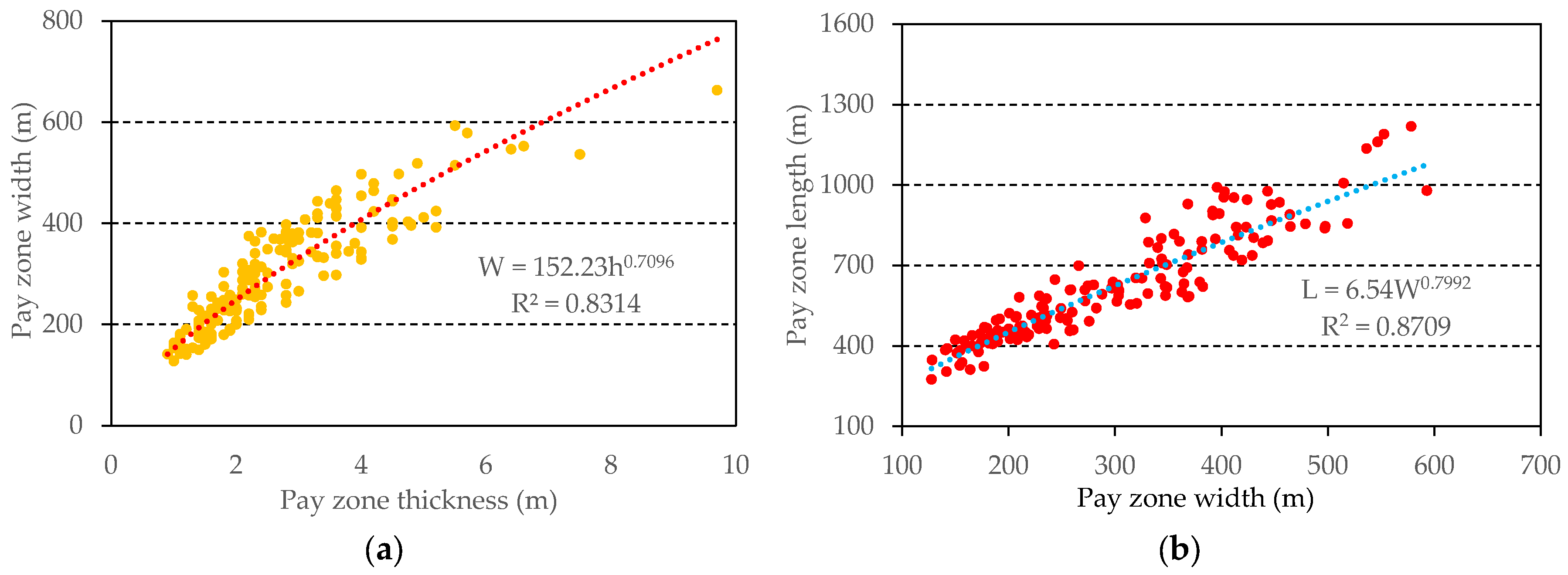
Through fitting the geometric parameter sample data of effective sand bodies in tight sandstone gas reservoirs in Ordos Basin, the correlations of the pay zone length and width with the pay zone thickness were obtained (Figure 2):

$$W=152.23h^{0.7096}$$

(1)

$$L=6.54W^{0.7992}$$

(2)

where W is the pay zone width, m; h is the pay zone thickness, m; L is the pay zone length, m.

For a multi-layer commingled well, the top pay zone is taken as the reference layer, and from top to bottom, the pay zone width ratio of each pay zone can be calculated using Equation (3):

$${\displaystyle \frac{W_k}{W_1}}={({\displaystyle \frac{h_k}{h_1}})}^{0.7098}$$

(3)

where k is the k-th pay zone that is perforated for production in a gas well, dimensionless.

The thickness of each pay zone of a gas well can be easily determined from the well loggings, and yet the widths and lengths of pay zones cannot be accurately measured. With the known thickness of each pay zone of a gas well, the lengths and widths of pay zones can be estimated using Equations (1) and (2). However, the estimation of lengths and widths of pay zones only by Equations (1) and (2) still could not meet the accuracy requirement. Hence, to improve the accuracy of the calculated lengths and widths of pay zones, the width ratios among pay zones and the ratios of length to width of each pay zone are first calculated using Equations (2) and (3), and then the length and width of each pay zone are further calculated by substituting the production data.

2.3. Flowing Bottom-Hole Pressure

To determine the gas production of each pay zone in a gas well, one first needs to calculate the flowing bottom-hole pressure of each pay zone according to the wellhead tubing pressure. The flowing bottom-hole pressure calculation equations are based on the classic method [23].

For a gas well brought into production, the flowing bottom-hole pressure of pay zones at an arbitrary moment (j > 1) can be calculated using Equation (4):

$$P_{wjk}=\sqrt{{P_{tj}}^2{e}^{2C_j}+{\displaystyle \frac{1.324\times {10}^{-10}{(\overline{T}{\overline{Z}}_j{q}_{mj})}^2{f}_j}{d^5}}(e^{2C_j}-1)}$$

(4)

$$C_j={\displaystyle \frac{0.03415r_g{H}_k}{\overline{T}{\overline{Z}}_j}}$$

(5)

$$f_j={\left(1.114-2\lg ({\displaystyle \frac{\epsilon }{d}}+{\displaystyle \frac{21.25}{{\mathrm{Re}}_j}})\right)}^{-2}$$

(6)

$${\mathrm{Re}}_j={\displaystyle \frac{1.776\times {10}^{-2}{q}_{mj}{r}_g}{d{\overline{u}}_j}}$$

(7)

where j represents the production time (days), dimensionless; P_w is the flowing bottom-hole pressure, MPa; P_t is the wellhead tubing pressure of a gas well, MPa; $\overline{T}$ is the average temperature inside the production tubing, K; $\overline{Z}$ is the Z factor at the average tubing pressure, dimensionless; q_m is the measured wellhead daily gas production, m³/d; H is the reservoir middle depth, m; f is the friction coefficient of the production tubing inside wall, dimensionless; $\epsilon$ is the roughness of the production tubing inside wall (often taken as 1.6 × 10⁻⁵), m; d is the inside diameter of the production tubing, m; Re is the Reynolds number of fluid flow inside the production tubing, dimensionless; r_g is the relative density of natural gas (often taken as 0.62 under the standard conditions), dimensionless; $\overline{\mu }$ is the average viscosity of natural gas in the production tubing, mPa·s.

The average temperature inside the production tubing is calculated by using Equation (8):

$$\overline{T}={\displaystyle \frac{T_w+T_t}{2}}$$

(8)

where T_w is the bottom-hole temperature of the gas well, K; T_t is the wellhead temperature of the gas well, K.

The average pressure inside the production tubing is approximated empirically using Equation (9) [24]:

$${\overline{P}}_{tj}={\displaystyle \frac{2}{3}}(P_{w(j-1)}+{\displaystyle \frac{{P_{tj}}^2}{P_{tj}+P_{w(j-1)}}})$$

(9)

where $\overline{P_t}$ is the average pressure inside the production tubing, MPa.

The initial flowing bottom-hole pressure of pay zones in a gas well is computed empirically by using Equation (10) [24]:

$${\left.P_{wjk}\right|}_{j=1}=(1+8.2\times {10}^{-5}{H}_k){\left.P_{tj}\right|}_{j=1}$$

(10)

The flowing bottom-hole pressure of each pay zone at an arbitrary moment is then calculated by substituting the initial flowing bottom-hole pressure of pay zones into Equations (4)–(10) for recursive calculation.

2.4. Seepage Equation

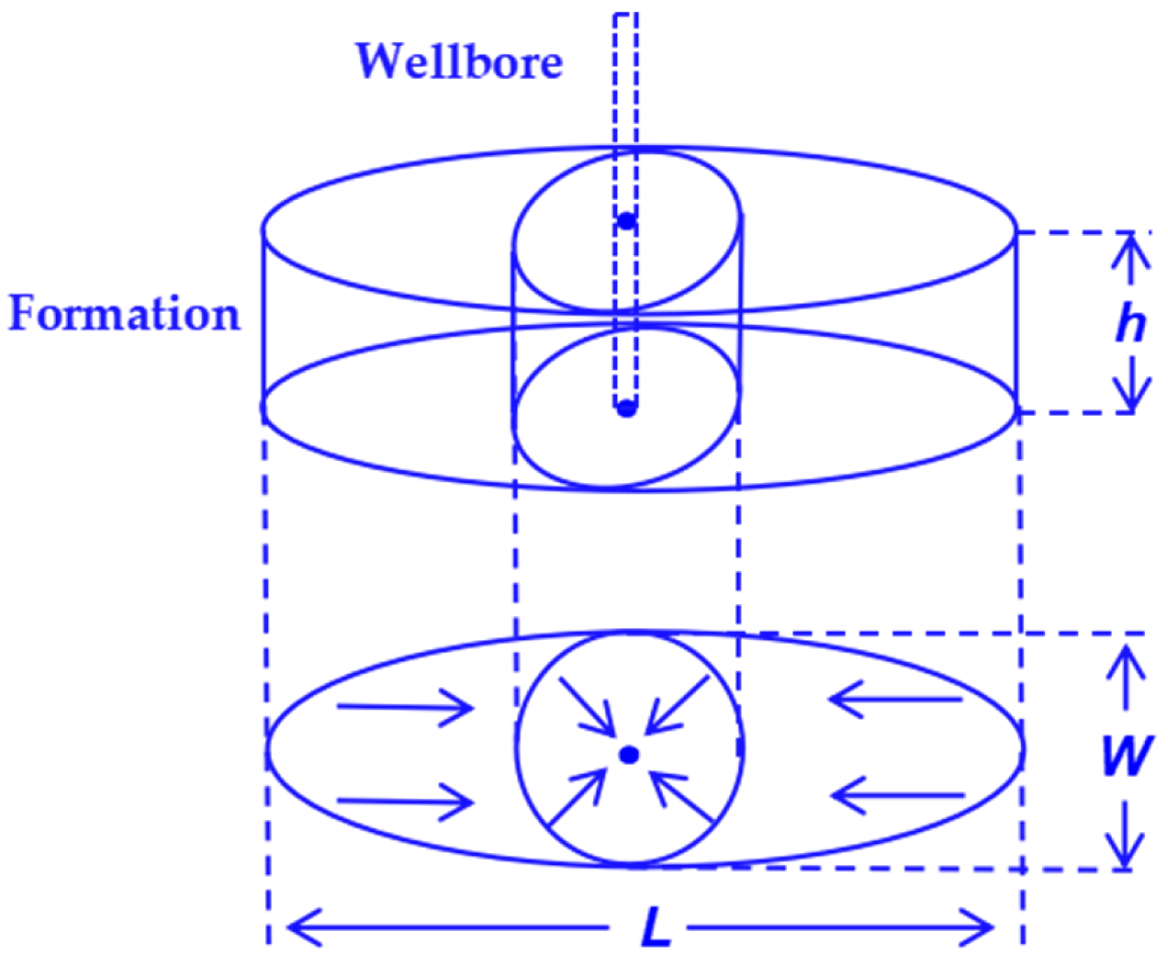
As stated by Li et al. [25,26], the fluid seepage within the elliptical boundary can be simplified into the radial flow in the near-wellbore zone and the linear flow in the zone far away from the wellbore (Figure 3).

$$q_{jk}={\displaystyle \frac{{\tau }_j}{24}}\cdot {\displaystyle \frac{-A_{jk}+\sqrt{A_{jk}^2+4A_{jk}(P_{jk}^2-P_{wjk}^2)}}{2B_{jk}}}$$

(11)

$$A_{jk}=11.57{\displaystyle \frac{\mu Z_{jk}{T}_k{P}_{sc}}{2\pi K_{gk}{h}_k{Z}_{sc}{T}_{sc}}}\ln ({\displaystyle \frac{W_k}{2r_w}})$$

(12)

$$B_{jk}=1.3396\times {10}^{-16}{\displaystyle \frac{M{r}_g\beta Z_{jk}{T}_k}{R{r}_w}}{({\displaystyle \frac{P_{sc}}{2\pi h_k{Z}_{sc}{T}_{sc}}})}^2$$

(13)

$$\beta ={\displaystyle \frac{9.638\times {10}^{10}}{K_{gk}^{0.934}}}$$

(14)

where q is the gas production rate, m³/d; τ is the daily production hours of a gas well, h; P is the reservoir pressure, MPa; M is the molecular weight of natural gas, kg/kmol; β is the gas turbulence factor for high-speed flow, m⁻¹; T is the formation temperature, K; Z is the Z factor of natural gas, dimensionless; R is the universal gas constant (typically equal to 0.008314), MPa·m³/(kmol K); r_w is the wellbore radius, m; P_sc is the standard condition pressure, MPa; T_sc is the standard condition temperature, K; Z_sc is the Z factor of natural gas under the standard conditions, dimensionless; μ is the natural gas viscosity, mPa·s; K_g is the effective permeability of the gas phase, mD.

After the pressure drop reaches the seepage boundary, the fluid flow inside the reservoir can be approximated as the composite flow consisting of the near-wellbore radial flow and the remote linear flow. The corresponding seepage equations are as follows:

$$q_{jk}={\displaystyle \frac{{\tau }_j}{24}}\cdot {\displaystyle \frac{-a_{jk}+\sqrt{a_{jk}^2+4a_{jk}(P_{jk}^2-P_{wjk}^2)}}{2b_{jk}}}$$

(15)

$$a_{jk}=11.57{\displaystyle \frac{\mu Z_{jk}{T}_k{P}_{sc}}{K_{gk}{h}_k{Z}_{sc}{T}_{sc}}}\left({\displaystyle \frac{1}{2\pi }}\ln ({\displaystyle \frac{W_k}{2r_w}})+{\displaystyle \frac{(L_k-W_k)}{2W_k}}\right)$$

(16)

$$b_{jk}=1.3396\times {10}^{-16}{\displaystyle \frac{M{r}_g\beta Z_{jk}{T}_k}{R}}{({\displaystyle \frac{P_{sc}}{h_k{Z}_{sc}{T}_{sc}}})}^2\left({\displaystyle \frac{1}{4{\pi }^2{r}_w}}+{\displaystyle \frac{(L_k-W_k)}{2{W_k}^2}}\right)$$

(17)

The critical time when the production pressure drop reaches the seepage boundary is calculated below [27]:

$$t_{ck}=0.73{\displaystyle \frac{{\phi }_k{\mu }_i{C}_{tk}{W_k}^2}{K_{gk}}}$$

(18)

where t_c is the critical time when the production pressure drop arrives at the seepage boundary, d; φ is the porosity of the pay zone, dimensionless; μ_i is the natural gas viscosity under the initial reservoir pressure, mPa·s; C_t is the comprehensive elastic compressibility of rocks (often taken as 0.02 for gas reservoirs), MPa⁻¹.

Hence, the daily gas production of a gas well at an arbitrary time can be written as:

$$Q_j={\displaystyle \sum _1^n{q}_{jk}}$$

(19)

where Q is the daily gas production of a gas well, m³/d; n is the number of pay zones in a gas well, dimensionless.

The cumulative gas production of each pay zone at an arbitrary time can be written as:

$$N_{jk}={\displaystyle \sum _1^j{q}_{jk}}$$

(20)

The current cumulative gas production of a gas well is:

$$U_J={\displaystyle \sum _1^J{Q}_j}$$

(21)

where U is the cumulative gas production of a gas well, m³.

2.5. Reservoir Pressure

Provided that the width of the top pay zone of a gas well is W₁ and the thickness of each layer is measured, the widths of other pay zones can be calculated using Equation (3), and their lengths can be estimated using Equation (2). The dynamic reserves of each pay zone can be calculated by substituting the length and width of each pay zone into Equation (22).

$$G_k={\displaystyle \frac{\pi L_k{W}_k{h}_k{\phi }_k{S}_{gik}}{40000B_{gik}}}$$

(22)

where G is the dynamic reserves of a pay zone, 10⁴ m³; S_gi is the initial gas saturation of the pay zone, dimensionless; B_gi is the natural gas volume factor under the initial reservoir pressure, dimensionless.

Based on the material balance equation, the reservoir pressure of the k-th pay zone of a gas well at an arbitrary time can be solved:

$${\displaystyle \frac{P_{(j+1)k}}{Z_{(j+1)k}}}={\displaystyle \frac{P_{ik}}{Z_{ik}}}(1-{\displaystyle \frac{N_{jk}}{G_k}})$$

(23)

2.6. Computation Workflow

During the model computation, the reservoir pressure, flowing bottom-hole pressure, and production rates of pay zones all vary with time sequences. Moreover, the calculation results of the previous time step are used as the input parameters for the calculation of this next time step. Therefore, the stepwise recursive computation based on time sequences (Figure 4) is performed to accomplish the production allocation of gas wells. The detailed steps of computation are as follows:

① Assume the initial value to the top pay zone width W₁. Substitute the thicknesses of pay zones h_k and W₁ into Equation (3) to calculate the widths of other pay zones W_k and then calculate the lengths of pay zones using Equation (2). Subsequently, the dynamic reserves of each pay zone Gk will be calculated using Equation (22).

② Substitute the wellhead tubing pressure P_tj of the gas well into Equations (4)–(10) and recursively calculate the flowing bottom-hole pressure of pay zones P_wjk.

③ Use Equation (18) to calculate the critical time t_ck when the production pressure drops of pay zones reach the corresponding seepage boundaries.

④ Before the production pressure drop reaches the seepage boundary (j ≤ t_ck), substitute the flowing bottom-hole pressure P_wjk and reservoir pressure P_jk of each pay zone into Equation (11) to calculate the daily gas production of pay zones q_jk. After the production pressure drops reach the seepage boundary (j > t_ck), substitute the flowing bottom-hole pressure P_wjk and reservoir pressure P_jk of each pay zone into Equation (15) to calculate the daily gas production of pay zones q_jk.

⑤ Use Equation (20) to calculate the cumulative gas production of each pay zone N_jk.

⑥ Substitute the dynamic reserves G_k and cumulative gas production N_ik of each pay zone into Equation (23) to calculate the reservoir pressure of pay zones P_(j+1)k at the next time step (j + 1).

⑦ Substitute the flowing bottom-hole pressure of pay zones P_wjk calculated at Step ②, and reservoir pressure of pay zones P_(j+1)k obtained at Step ⑥ into Equation (11) or (15) to compute the daily gas production of pay zones q_(j+1)k at the next time step.

⑧ Repeat Steps ③–⑦ to determine the reservoir pressure P_jk and daily gas production q_jk of each pay zone of the gas well at an arbitrary time.

⑨ Determine the cumulative gas production of the gas well using Equation (21). The assigned value of W₁ is considered an appropriate value of the top pay zone width if the error between the calculated cumulative production of the gas well U_J and the measured cumulative production of the well U_m is less than 5% (this value can be properly adjusted according to the accuracy requirement), and the consistent trends are observed for the calculated and measured daily gas production. Otherwise, a new value shall be assigned to W₁ until the fitting accuracy meets the above requirement.

3. Model Validation and Analysis

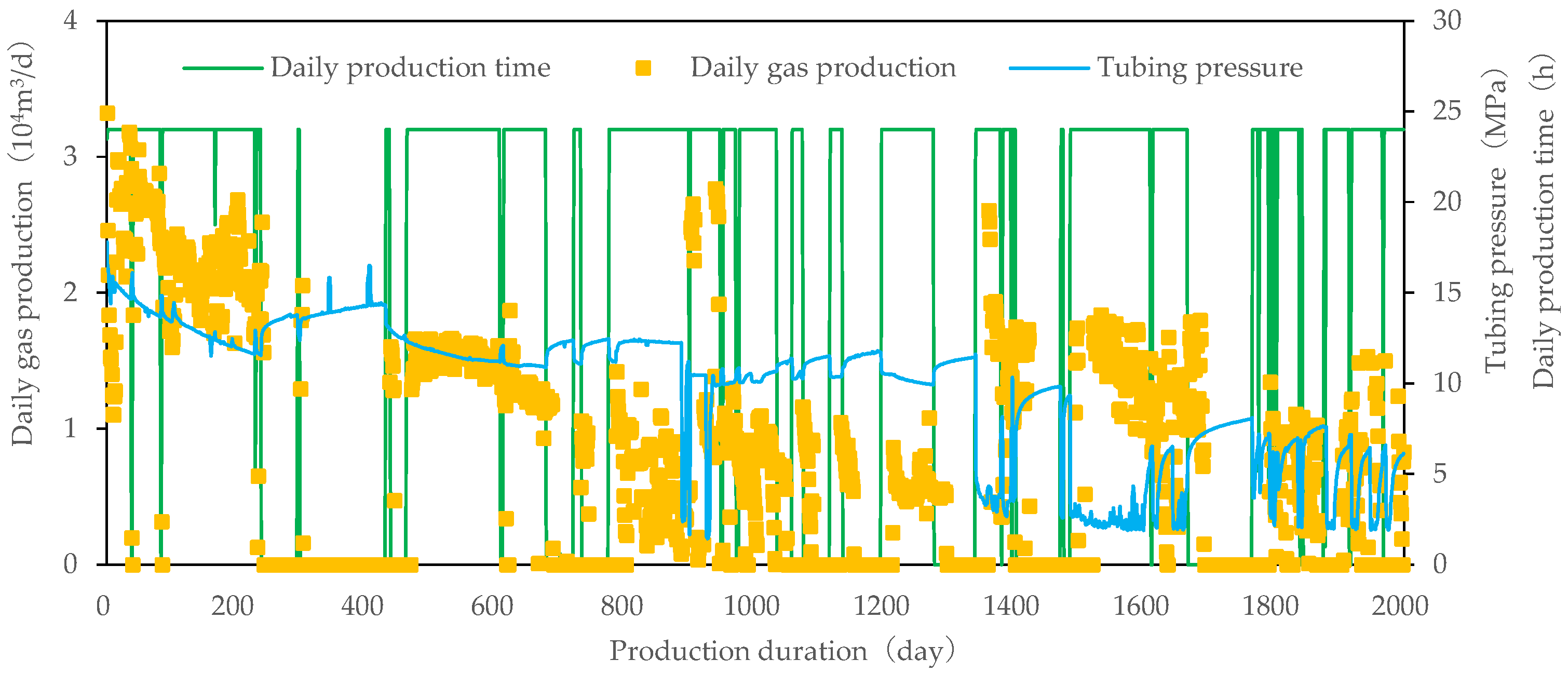
The gas wells in the Sulige gas field with available production profile logging data were chosen to validate the reliability of the new model. Here, a case study of Well SDJ4-W is presented. Vertically, this well has three pay zones that are producing at the same time (two in He-VIII Member of the Shihezi Formation and one in Shan-I Member of the Shanxi Formation). The pipe string and reservoir parameters are shown in

Table 1. Reservoir and pipe string parameters of Well SDJ4-W.

Parameters		The 1st Pay Zone	The 2nd Pay Zone	The 3rd Pay Zone
Reservoir parameters	Pay zone thickness (m)	2.3	3.2	5.1
	Porosity	10.6%	7.4%	7.6%
	Gas saturation	53.8%	61.2%	57.9%
	Permeability (mD)	0.65	0.27	0.43
	Initial reservoir pressure (MPa)	26.4	26.6	26.8
	Reservoir temperature (K)	378.15
Column parameters	Pay zone depth (m)	3069.4	3089.5	3117.85
	Casing pressure (MPa)	Shown in Figure 5

, and the production data are displayed in Figure 5. All these data were obtained from well-logging and field monitoring

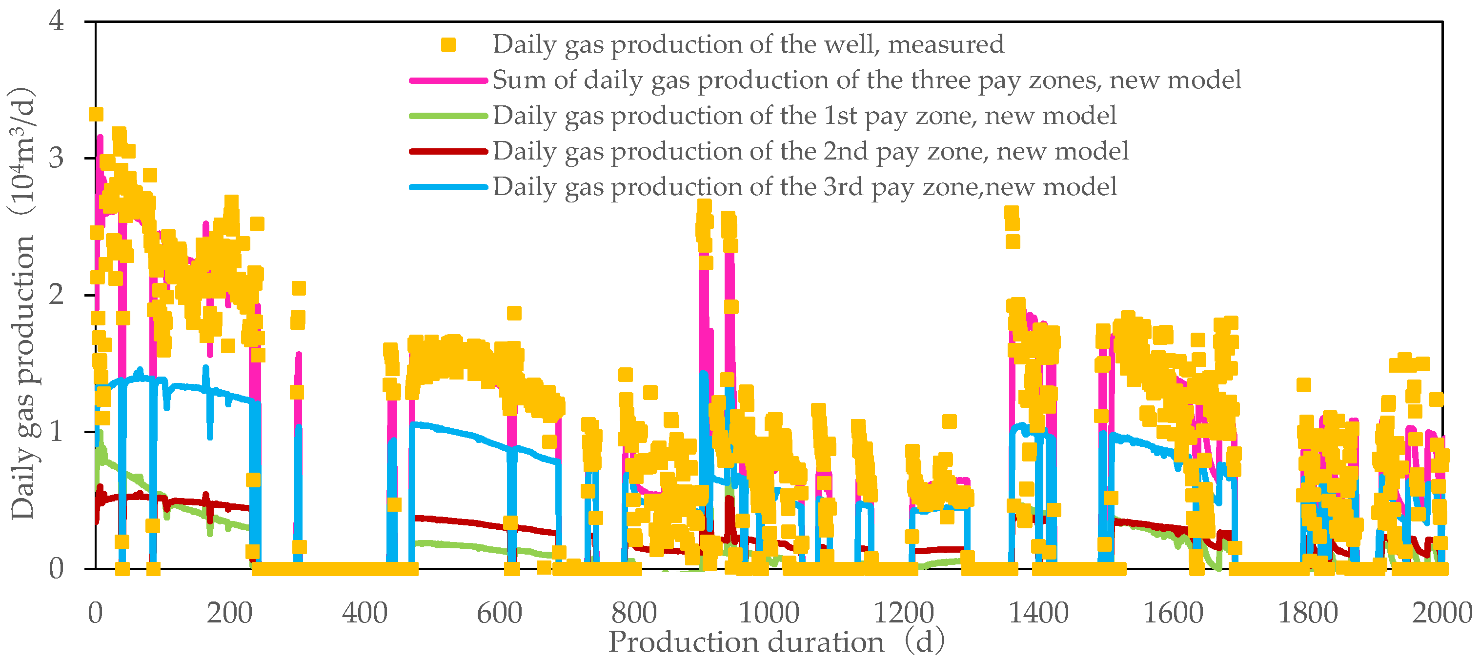
Production allocation was performed according to the computation workflow in Figure 4 for Well SDJ4-W. The sum of daily gas production of the three pay zones obtained by the new model presents a consistent trend with the measured daily gas production (Figure 6), and the calculated and measured cumulative gas production are 1.58 × 10⁷ m³ and 1.60 × 10⁷ m³, respectively, with an error of 0.89% (<5%, the required fitting accuracy), when the width of the top pay zone of the gas well is adjusted to W₁ = 275.1 m. Furthermore, the calculated widths of the three pay zones are 275.1 m, 347.7 m, and 484.5 m, associated with the lengths of 552.9 m, 666.8 m, and 868.6 m, respectively. The drainage areas are 0.12 km², 0.18 km² and 0.33 km², respectively, corresponding to the dynamic reserves of 3.34 × 10⁶ m³, 5.68 × 10⁶ m³ and 1.71 × 10⁷ m³. The production data of the gas well were also input into the Blasingame production decline curve for fitting. The estimated drainage area and dynamic reserves of the well are 0.28 km² and 2.69 × 10⁷ m³, respectively. It is shown that the overall drainage area of the gas well lies among those of the three pay zones and the total dynamic reserves of the well present a small error of only 3.1% compared to the sum of the dynamic reserves of the three pay zones. Hence, the model is reliable.

It was shown in Figure 6 that among the three pay zones, the third (bottom) pay zone contributes the highest gas production. It is obvious that the third pay zone has the largest dynamic reserves due to its large net pay thickness, drainage area, porosity, and gas saturation. Therefore, this pay zone maintains relatively high reservoir pressure during the well production, according to Equation (23). In addition, this pay zone has relatively low fluid flow resistance because of its relatively high permeability. Because of the larger reservoir pressure and lower fluid flow resistance, this pay zone has the highest gas production among the three pay zones. The medium gas production of the second (middle) pay zone and the least one of the first (top) pay zone can be explained likewise. It should be noted that the first pay zone presents initial gas production rates higher than those of the second pay zone due to the larger permeability and, hence, lower fluid flow resistance of the first zone. However, the small thickness, drainage area, and gas saturation of the first pay zone lead to lower dynamic reserves. As suggested by the material balance equation, the reservoir pressure of the first pay zone drops fast during the well production, and it cannot maintain high production. Instead, its gas production declines rapidly. On Day 121, after being brought into production, the gas production rate of the first pay zone is exceeded by that of the second pay zone, and the ultimate contributions of the first pay zone to the cumulative gas production of the well are the least among these three pay zones. Higher permeability may lead to higher initial gas production of pay zones. Yet, in view of the life span of gas wells, the ultimate gas production contributions of pay zones are affected jointly by multiple factors such as permeability and dynamic reserves. Permeability decides fluid flow resistance, while dynamic reserves affect the preservation of reservoir pressure.

In fact, equations of the new model have already shown how sensitive the production allocation is to key parameters like reservoir physical properties and pressure. Equation (23) demonstrates that reservoir pressure is influenced by both the initial reservoir pressure and dynamic reserves. Specifically, higher initial reservoir pressure and greater dynamic reserves contribute to maintaining a higher reservoir pressure. Furthermore, Equation (22) indicates that dynamic reserves are directly proportional to parameters such as net pay thickness, porosity, and saturation. In addition, according to seepage Equations (11) and (15), the higher the permeability, the lower the seepage resistance and the higher the gas productivity. In summary, the production contribution rate of each pay zone is highly sensitive to the inputs of the new model, including initial reservoir pressure, net pay thickness, porosity, permeability, and saturation. These parameters directly influence production allocation outcomes. Therefore, it is imperative to ensure the accuracy of these inputs prior to conducting production allocation.

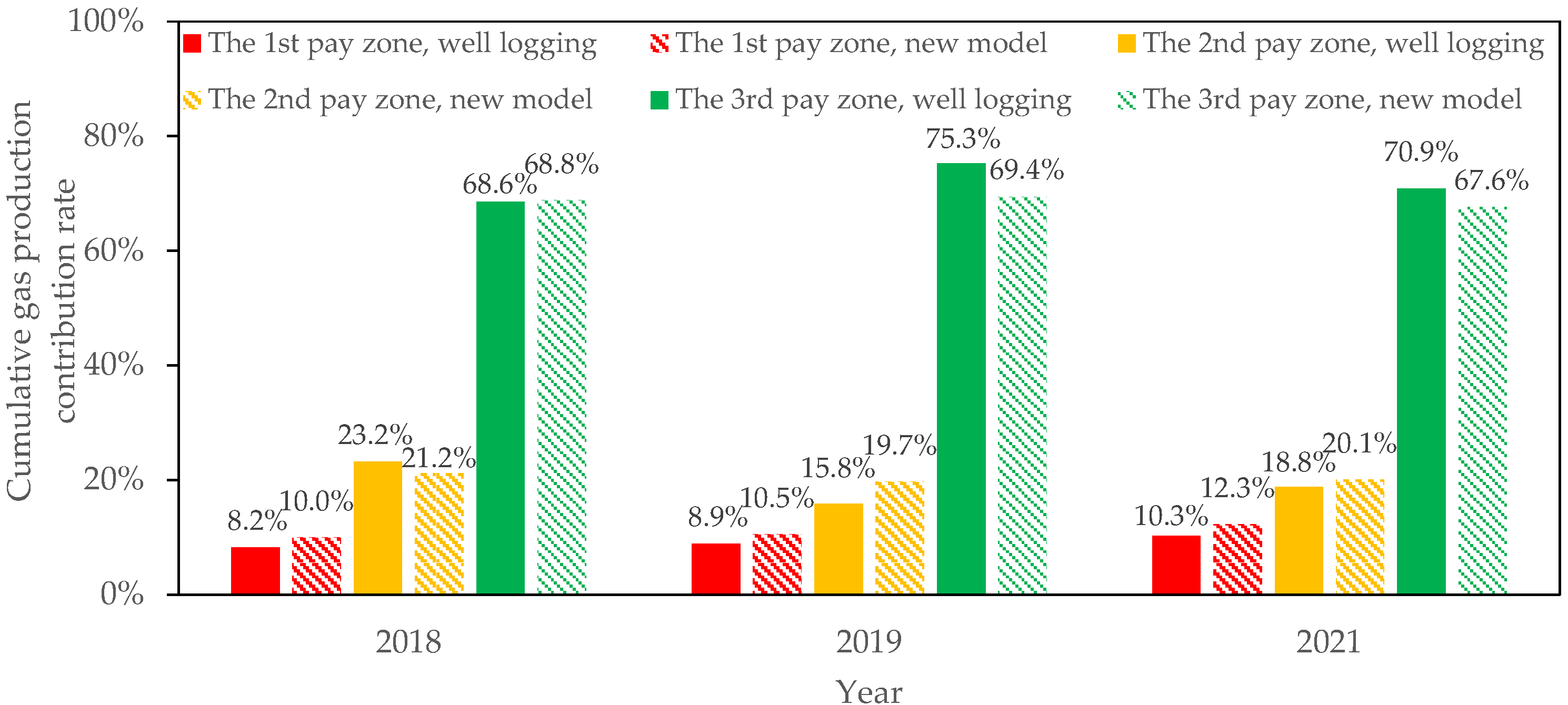
Production profile logging was performed for Well SDJ4-W in 2018, 2019, and 2021, respectively. The cumulative gas production contributions of the pay zones based on the new model are fairly close to the ones based on production profile logging, with the largest error smaller than 10%, which also demonstrates the reliability of the proposed production allocation model (Figure 7). The calculation error (smaller than 10%) primarily stems from the fluctuation in production data and measurement errors of inputs. Despite these uncertainties, the overall fluctuation in production data and measurement errors of inputs are generally limited; their influence on the outcome of production allocation is acceptable.

The Formation Coefficient Method (Kh Method) [28] was applied to the calculation of cumulative gas production contributions of pay zones, and the calculation results were compared with the results of the new model and production profile logging (Figure 8). The calculation errors of the Formation Coefficient Method are much higher than those of the new model because, in the Formation Coefficient Method, the weighted calculation of gas production contributions is rather simple, based solely on the Kh values of pay zones. For instance, the first pay zone is thin but has higher permeability, so the product of K and h is high, and the gas production contributions are severely overestimated by the Formation Coefficient Method. On the contrary, the presented production allocation model is based on seepage mechanics and couples multiple factors, such as the reservoir properties, effective sand body geometric parameters, reservoir pressure, wellbore pressure, and gas production rates. It delivers results that are much more accurate and reliable. Although the Formation Coefficient Method can obtain the production allocation results more simply and quickly, by programming the formulas of the new model into software, the rapid calculation of production allocation can also be achieved. Compared with the production profile logging, the software can obtain the production allocation results even faster and cheaper.

To validate the new model further, it was applied to another five gas wells from the Ordos Basin, which have production profile logging data. These wells include three in Block A (W1, W2, W3) and two in Block B (Y1, Y2). Compared with Block B, Block A has better reservoir physical properties and a larger net pay thickness. The calculated results from the new model closely match those obtained from production profile logging, with overall errors in production contribution rates remaining below 10% (

Table 2. Comparison of production allocation results between the new model and production profile logging for five additional gas wells from Ordos Basin.

Well Name	Depth (m)	Porosity	Gas Saturation	Permeability (mD)	Net Pay Thickness (m)	Cumulative Production Contribution Ratios		Errors
						Production Profile Logging	New Model
W1	3040.1	11.5%	59.6%	1.89	4.2	68.3%	73.4%	5.1%
	3097.8	6.5%	49.4%	0.50	1.9	13.1%	9.7%	−3.4%
	3115.5	6.5%	50.5%	0.31	2.5	18.6%	17.0%	−1.6%
W2	3141.7	11.6%	47.4%	1.28	3.1	36.6%	41.8%	5.2%
	3170.0	7.1%	46.5%	0.20	3.7	43.6%	41.2%	−2.4%
	3225.7	6.5%	40.3%	0.35	5.4	19.8%	17.0%	−2.8%
W3	3007.2	8.7%	57.9%	0.55	3.3	17.6%	19.7%	2.1%
	3063.5	12.1%	64.3%	1.05	5.0	70.1%	74.3%	4.2%
	3091.0	10.2%	52.0%	0.55	1.9	12.3%	6.0%	−6.3%
Y1	3139.5	9.2%	50.0%	0.54	3.9	38.1%	46.2%	8.1%
	3209.6	8.4%	56.0%	0.35	4.2	61.9%	53.8%	−8.1%
Y2	3007.2	3187.4	12.2%	52.3%	1.4	37.8%	44.1%	6.3%
	3063.5	3230.4	8.9%	66.1%	0.25	62.2%	55.9%	−6.3%

). This indicates that the new model is still reliable for gas wells with different geological conditions.

4. Field Application

Numerical simulation is one of the most classical methods for remaining gas distribution prediction and well placement, but the numerical simulation of tight gas reservoirs has a high dependency on accurate geological models. High-precision geological modeling of tight gas reservoirs is difficult to complete because of its strong heterogeneity. The new model, which is accurate and reliable, provides a supplement for remaining gas distribution prediction and well placement.

The SZ block is located in the central Sulige gas field. The He-VIII Member and Shan-I Member are the main development layers. This block has favorable reservoir physical properties, and the average gas abundance reaches 1.6 × 10⁸ m³/km². The development of this block started in 2003, and by the end of 2022, 941 gas wells have been brought into production, including 715 vertical wells and 226 horizontal wells. The well density is about 2.1 wells/m². By far, the cumulative gas production is 1.71 × 10¹⁰ m³, corresponding to a recovery factor of 28.0%.

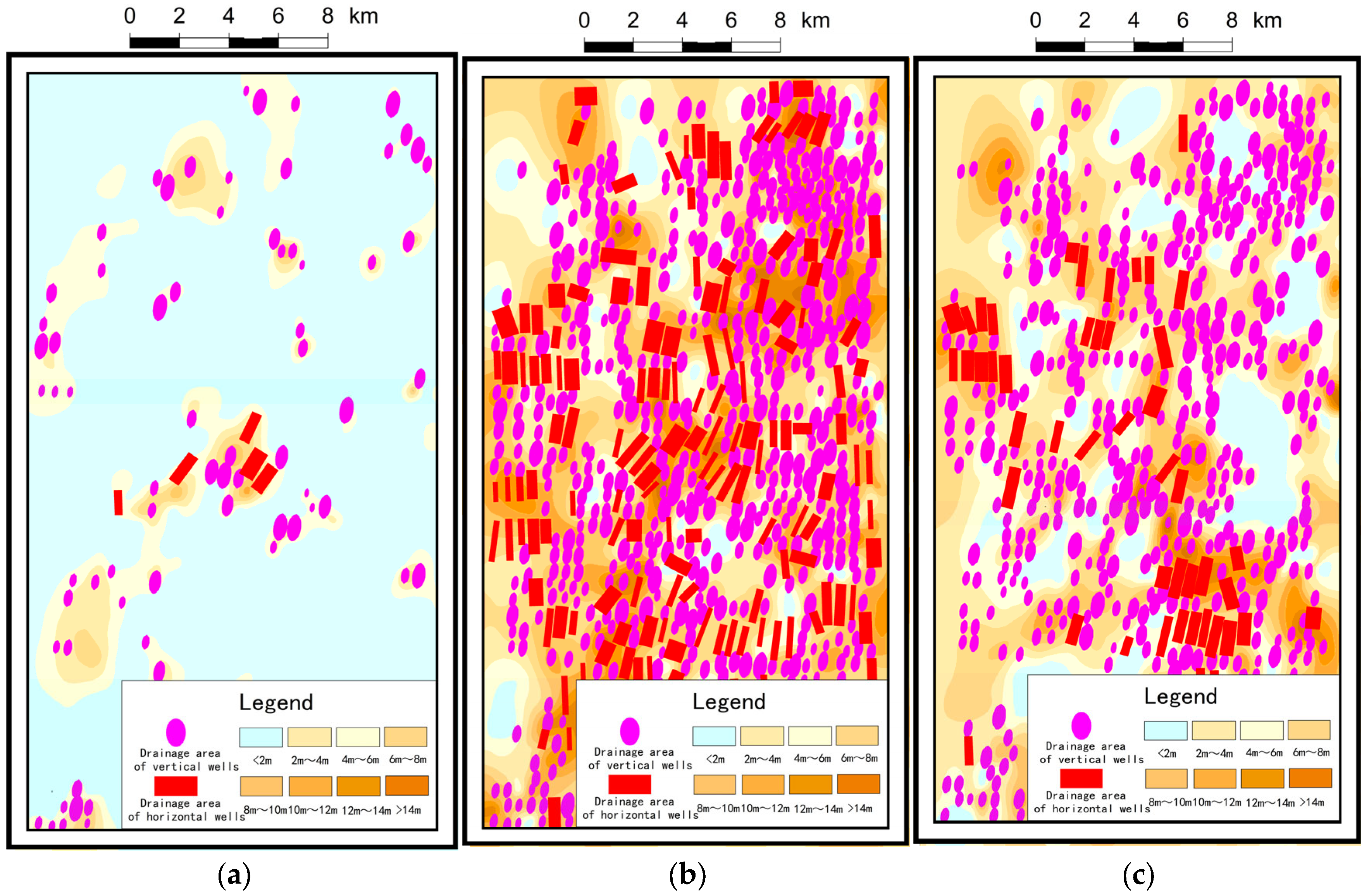
Based on the new model presented in this paper, production allocation was performed for 715 vertical wells in this block. The lengths and widths of pay zones of the vertical wells were calculated by using the new model, and the seepage ellipses of pay zones of the vertical wells were drawn based on the well coordinates. For horizontal wells, the classic Blasingame production decline curve was used to compute the drainage areas. By performing this, the reserve recovery and remaining gas distribution of each pay zone are clearly visualized (Figure 9). To simplify the computation workflow, the pay zones were vertically divided into three, namely the Upper He-VIII Member, Lower He-VIII Member, and Shan-I Member. More pay zones can also be divided vertically according to the required resolutions of production allocation.

The fine evaluation of the dynamic reserves, drainage areas, recovery factors, and remaining reserves of pay zones of the SZ block was delivered based on the production allocation results (

Table 3. Production allocation results of gas wells in the SZ block, the Sulige gas field.

Formation	Vertical Wells				Horizontal Wells				Producing Reserves (109 m3)	Remaining Reserves (109 m3)
	Number of Wells	Average Dynamic Reserves (106 m3)	Average Drainage Area (km2)	Cumulative Production (109 m3)	Number of Wells	Average Dynamic Reserves (106 m3)	Average Drainage Area (km2)	Cumulative Production (109 m3)
Upper He-VIII	79	11.92	0.23	0.73	5	51.90	0.71	0.17	3.19	2.30
Lower He-VIII	626	20.12	0.26	6.26	145	58.30	0.81	4.62	36.62	25.74
Shan-I	505	12.35	0.25	3.83	47	54.75	0.75	1.50	21.18	15.85
Sum/Average	715	30.28	0.25	10.82	226	57.31	0.79	6.29	60.99	43.89

). In the SZ block, the cumulative gas production of the Upper He-VIII, Lower He-VIII, and Shan-I Members is 8.90 × 10⁸ m³, 1.09 × 10¹⁰ m³, and 5.33 × 10⁹ m³, respectively (the sum of cumulative gas production of vertical wells and horizontal wells of each formation), corresponding to the recovered factors of 27.9%, 29.7% and 25.2%, and the remaining reserves are 2.30 × 10⁹ m³, 2.57 × 10¹⁰ m³ and 1.58 × 10¹⁰ m³, respectively. The new model can be applied to field decision-making. In Figure 9, thick gas layers between the drainage areas of vertical and horizontal wells are the areas where the remaining gas is concentrated, which provides a reference for the next well placement. In the future, the infilling vertical wells may be deployed for the stacking enrichment zones of the remaining gas of the Lower He-VIII and Shan-I Members, while infilling horizontal wells may be deployed for the separate enrichment zones of the remaining gas of the Lower He-VIII and Shan-I Members to enhance gas recovery of the SZ block.

5. Conclusions

Based on the careful consideration of geometric parameters of effective sand bodies, wellbore pressure equation, material balance equation, and seepage equation with the elliptical boundary, this paper developed a new production allocation model of multi-layer commingled wells, applicable to tight sandstone gas reservoirs in the Ordos Basin. The new model was validated and applied to field cases. The following conclusions were drawn:

(1)

The gas production contributions of pay zones based on the new model are fairly close to the measurements of the production profile logging, with errors less than 10%. The production allocation results of the new model are more accurate and reliable than those of the Formation Coefficient Method since the new model has more thorough considerations and couples multiple parameters such as pressure, production rates, reservoir physical properties, and geometric parameters of effective sand bodies.

(2)

The overall drainage area of a gas well lies among those of each pay zone, and the total dynamic reserves of the well are close to the sum of the dynamic reserves of pay zones.

(3)

Higher permeability may lead to higher initial gas production of the pay zone, but the ultimate gas production contributions of pay zones are affected jointly by permeability and dynamic reserves. Permeability affects fluid flow resistance, and dynamic reserves impact the preservation of reservoir pressure in pay zones.

(4)

The new model has been successfully applied to the SZ block of the Sulige gas field, in which the fine evaluation of dynamic reserves, drainage areas, gas production, recovery factors, and remaining gas distributions of the Upper He-VIII Member, Lower He-VIII Member, and Shan-I Member was delivered. The application results provide technical support for the future well placement and enhanced gas recovery of the block.