Wind Power Prediction Method Based on Physics-Guided Fusion and Distribution Constraints

Abstract

Accurate wind power prediction is of great significance for grid stability and renewable energy integration. Addressing the challenge of effectively integrating physical mechanisms with data-driven methods in wind power prediction, this paper innovatively proposes a two-stage deep learning prediction framework incorporating physics-guided fusion and distribution constraints, aiming to improve the prediction accuracy and physical authenticity of individual wind turbines. In the first stage, we construct a baseline model based on multi-branch multilayer perceptrons (MLP) that eschews traditional attempts to accurately reconstruct complex three-dimensional spatiotemporal wind fields, instead directly learning the power conversion characteristics of wind turbines under specific meteorological conditions from historical operational data, namely the power coefficient (Cp). This data-driven Cp fitting method provides a physically interpretable and robust benchmark for power prediction. In the second stage, targeting the prediction residuals from the baseline model, we design a bidirectional long short-term memory network (BiLSTM) for refined correction. The core innovation of this stage lies in introducing Maximum Mean Discrepancy (MMD) as a regularization term to constrain the predicted wind speed-power joint probability distribution. This constraint enforces the model-generated power predictions to remain statistically consistent with historical real data distributions, effectively preventing the model from producing predictions that deviate from physical reality, significantly enhancing the model’s generalization capability and reliability. Experimental results demonstrate that compared to traditional methods, the proposed method achieves significant improvements in Mean Absolute Error, Root Mean Square Error, and other metrics, validating the effectiveness of physical constraints in improving prediction accuracy.

1. Introduction

In the current global context of actively promoting energy transition and vigorously developing renewable energy, wind power has become a key component of the energy structure due to its advantages of being clean and sustainable [1]. However, its output is influenced by meteorological conditions, exhibiting significant intermittency and volatility [2], posing tremendous challenges to the stable operation and precise dispatch of power systems. Conducting wind power prediction research has profound significance, as it can effectively address the uncertainty of wind power output, ensure reliable operation of power systems while enhancing their economic efficiency, and provide indispensable core support for large-scale wind power integration and national energy structure transformation [3].

Currently, input data, prediction models, and output data are the three core elements of wind power prediction [4]. For input data to prediction models, existing methods are generally constructed based on two types of data: historical measured generation power data and numerical weather prediction (NWP) data [5]. Accurate NWP data not only have relatively high costs and complex computational processes, but their prediction accuracy is also controversial, particularly as wind speed forecasts are susceptible to significant fluctuations with high noise and relatively low accuracy [6]. Meanwhile, the sparse distribution of meteorological stations often makes it difficult to obtain high-resolution spatial wind speed data [7]; historical power data is more suitable for short-term and ultra-short-term wind power generation prediction scenarios and has been widely applied [8]. How to effectively handle the adverse impact of high-noise wind speed forecast data on the accuracy and robustness of wind power prediction remains an important challenge in the field of wind power prediction [9].

Existing wind power prediction methods are mainly classified into four types: physical methods, statistical methods, artificial intelligence methods, and hybrid prediction methods [10]. Physical modeling methods typically refer to prediction methods based on physical principles and meteorological models. Physical models rely on NWP data to establish the relationship between wind speed and generation power, constructing NWP models to predict future wind speed and direction by simulating local climate conditions and boundary information through meteorological and geographical data [11], then using techniques such as wind power curves [12] to determine wind power. García-Santiago et al. [13] used the WRF model to evaluate the capability of Fitch wind farm parameterization and explicit wake parameterization schemes to predict wind farm power under different atmospheric stability conditions, demonstrating that this method can effectively predict wind farm generation while considering regional wind climate variations. Such models have high prediction accuracy and strong physical interpretability. However, this model has limitations in computational efficiency; due to the necessity of considering complex fluid dynamics laws and atmospheric phenomena [14], its feasibility in large-scale data scenarios is low. While approximate empirical physical models can provide qualitative reference for physical mechanism analysis, they are often difficult to accurately predict the generation of commercial-scale wind farms due to numerous simplifying assumptions and neglected physical phenomena [15]. Currently, scholars have proposed various empirical formulas for modeling power coefficients, but consensus has not yet been reached in academia on the solution selection that balances model flexibility and robustness [16]. Statistical methods are based on mathematical statistics theory, constructing mathematical models through curve fitting and parameter estimation on the basis of large amounts of historical data, such as the autoregressive moving average model (ARMA) [17], the autoregressive integrated moving average model (ARIMA) [18], etc. These methods are simple and practical, have been widely applied in short-term prediction with relatively mature technology, but have poor adaptability to nonlinear, abrupt wind power data, and insufficient long-term prediction accuracy. With the advent of the computer era, artificial intelligence methods have received more attention due to their ability to mine nonlinear relationships and deep features of training data. Support vector machines (SVM) [19], multilayer perceptrons (MLP) [20], convolutional neural networks (CNN) [21], long short-term memory networks (LSTM) [22], and other artificial intelligence models have been applied to wind energy prediction. Transformer architectures and their variants, such as Informer [23], Autoformer [24], and other attention mechanism-based models, have shown excellent performance in capturing long-term temporal dependencies. Additionally, graph neural networks (GNN) [25], spatiotemporal graph neural networks (ST-GNN) [26], and other methods have effectively utilized spatial correlations between wind farms. Ensemble learning methods such as XGBoost [27], LightGBM [28], CatBoost [29], and other gradient boosting tree models have been widely applied in wind power prediction due to their efficiency and accuracy.

Single intelligent prediction models still have large prediction errors when dealing with highly volatile wind data. Therefore, many scholars have proposed combined prediction methods. Combined prediction methods significantly improve prediction accuracy while reducing model overfitting by combining multiple prediction models or integrating single prediction models with feature engineering, signal decomposition, error correction, and other strategies. Signal decomposition methods such as variational mode decomposition (VMD) [30], empirical mode decomposition (EMD) [31], ensemble empirical mode decomposition (EEMD) [32], and complete ensemble empirical mode decomposition with adaptive noise (CEEMDAN) [33] have been widely used to process non-stationary wind power series. Hou et al. [34] proposed a short-term wind power multi-step prediction model integrating CEEMDAN-VMD secondary decomposition, KPCA dimensionality reduction, ENAOA parameter optimization, BILSTM prediction, and error correction. Based on validation with data from northwest China wind farms, this model significantly reduced prediction errors compared to other single models. M.A. Hossain et al. [35] used a hybrid model composed of CNN layers, fully connected neural network layers, and gated recurrent unit layers to predict very short-term wind data.

It is worth noting that these purely data-driven models all have three core defects: (1) They ignore the aerodynamics, fluid mechanics, and other physical mechanisms in the wind energy conversion process, relying solely on data correlation modeling, which may generate prediction results that violate physical laws, leading to insufficient reliability in engineering applications; (2) Poor generalization ability in data-sparse regions (such as extreme weather, equipment start-stop transition phases), making it difficult to adapt to multi-condition changes in wind power systems; (3) The model is essentially a “black box” structure with insufficient interpretability, unable to clearly explain the physical meaning of prediction results. Meanwhile, the training process of data-driven models is prone to falling into local minima. Without guidance from wind power domain physical knowledge, it is difficult to achieve global optimal accuracy, and sufficient high-quality data support is required, with performance significantly degrading in scenarios with limited data acquisition.

To address the above issues, combining physical knowledge with deep learning has become an important research direction for improving the accuracy and reliability of wind power prediction [36]. Hybrid methods, as the core technical path in this direction, can effectively solve complex problems in wind power prediction by integrating physics-based methods with data-driven methods, featuring more transparent modeling processes and better cost-effectiveness. Currently, common strategies for combining physical principles with data-driven methods involve embedding physical constraints of wind power systems (such as Betz limit, power curve characteristics, etc.) into data preprocessing or model architecture design [37]. In recent years, Physics-Informed Neural Networks (PINN) have been widely applied in the field of wind power prediction [38], ensuring consistency between prediction results and wind power system physical laws by incorporating physical governing equations as regularization terms into the model learning process, significantly improving model reliability. The Tg-OFNN model proposed by Huang et al. [39] decomposes wind power into parts analytically resolved based on human knowledge and parts approximated through deep learning to integrate physical laws with data fitting capabilities. The team subsequently developed a prior-guided data-driven hybrid model [40], dividing prediction into one theory-guided stage and two data-driven stages, optimizing prediction results step by step. Zhang et al. [41] proposed a spatiotemporal wind field prediction method based on physics-informed deep learning, achieving spatiotemporal wind speed prediction for the entire wind field domain relying only on sparse LiDAR measurement data by embedding Navier–Stokes equations into deep neural networks. This method effectively combines measurement data with fluid physical laws, significantly improving prediction accuracy and reliability. Li et al. [42] developed a frequency-domain physics-informed neural network (FD-PINN) framework that integrates key physical models such as wind spectrum, wind field coherence functions, and wind profiles into deep neural networks. By introducing physical constraints in the frequency domain, it achieves accurate prediction of three-dimensional spatiotemporal wind fields at turbine locations, significantly improving the accuracy of spatial wind speed distribution prediction. To better utilize domain knowledge in wind power curves, Gao et al. [43] proposed a physics-constrained deep learning wind power prediction model TgDPF, which combines probability distribution knowledge of wind power curves with LSTM, ensures model differentiability through kernel density estimation (KDE), quantifies the difference between predicted and actual power distributions using JS divergence, effectively improving prediction robustness and accuracy under high-noise wind speeds. While such methods are effective, they typically fail to explicitly embed the core physical principles of wind energy conversion. This highlights a distinct research gap: the need for a more pragmatic framework that can effectively integrate fundamental physical principles into deep learning models, while avoiding reliance on overly complex equations or computationally expensive simulations.

Based on the above content, this paper proposes a novel physics-guided, two-stage prediction framework that synergistically combines the explanatory power of physical principles with the adaptive learning capabilities of deep neural networks. We intentionally term this approach “physics-guided” to clarify that our innovation lies in leveraging an established aerodynamic formula to architect the model, rather than attempting to solve complex fluid dynamics equations. The primary contribution of this work is not the invention of individual components (such as residual correction or MMD), but rather their novel synthesis into a cohesive framework designed specifically to overcome the limitations of end-to-end models in this physical context. The main innovations include:

• A Structured, Two-Stage Modeling Strategy: We decompose the complex, end-to-end prediction task into two more focused and individually optimizable sub-tasks. This “divide-and-conquer” architecture first establishes a physically grounded baseline and then performs a data-driven correction, a design choice aimed at enhancing both stability and accuracy.
• Physics-constrained baseline power prediction: In the first stage, we construct an independent deep neural network model specifically for predicting the wind turbine power coefficient (Cp). This method does not pursue accurate physical simulation of the wind field but directly learns the actual power conversion efficiency of wind turbines from massive SCADA data. This approach is closer to the actual operating characteristics of wind turbines and can effectively capture phenomena where performance deviates from theoretical curves due to factors such as equipment aging and environmental changes.
• Targeted Residual Correction with BiLSTM: The second stage is designed specifically to learn the complex, nonlinear error patterns of the physics-guided baseline model. By using a BiLSTM to model the residual sequence, we capture dynamic effects (like turbulence or control system lags) that are not accounted for in the first stage, allowing for a refined and highly accurate final prediction.
• Distributional Constraints for Physical Realism: We integrate the Maximum Mean Discrepancy (MMD) as a regularization term in the loss function. MMD is a mature distribution alignment technique, and its application here serves a specific purpose: to ensure that the joint probability distribution of the model’s predicted wind speed-power pairs statistically matches the distribution seen in historical data. This constrains the model to generate outputs that are not only accurate on average but also physically realistic, preventing the generation of “outlier” predictions that violate the system’s known operational characteristics.

The remainder of this paper is organized as follows. Section 2 introduces the overall structure of the prediction framework and the steps for making predictions. Section 3 presents experimental validation to demonstrate the effectiveness of the proposed method. Finally, Section 4 provides conclusions and future research prospects.

2. Materials and Methods

This research employs a two-stage hybrid model with deep integration of physical constraints for wind turbine generation prediction, addressing the challenges of high wind speed volatility and noise. In this section, we first introduce the overall framework, followed by a detailed elaboration of the three indispensable main components of the model, including the physics-based baseline model based on multi-branch multilayer perceptrons, the bidirectional LSTM residual correction model, and the MMD distribution regularization term.

2.1. Two-Stage Wind Power Prediction Structure

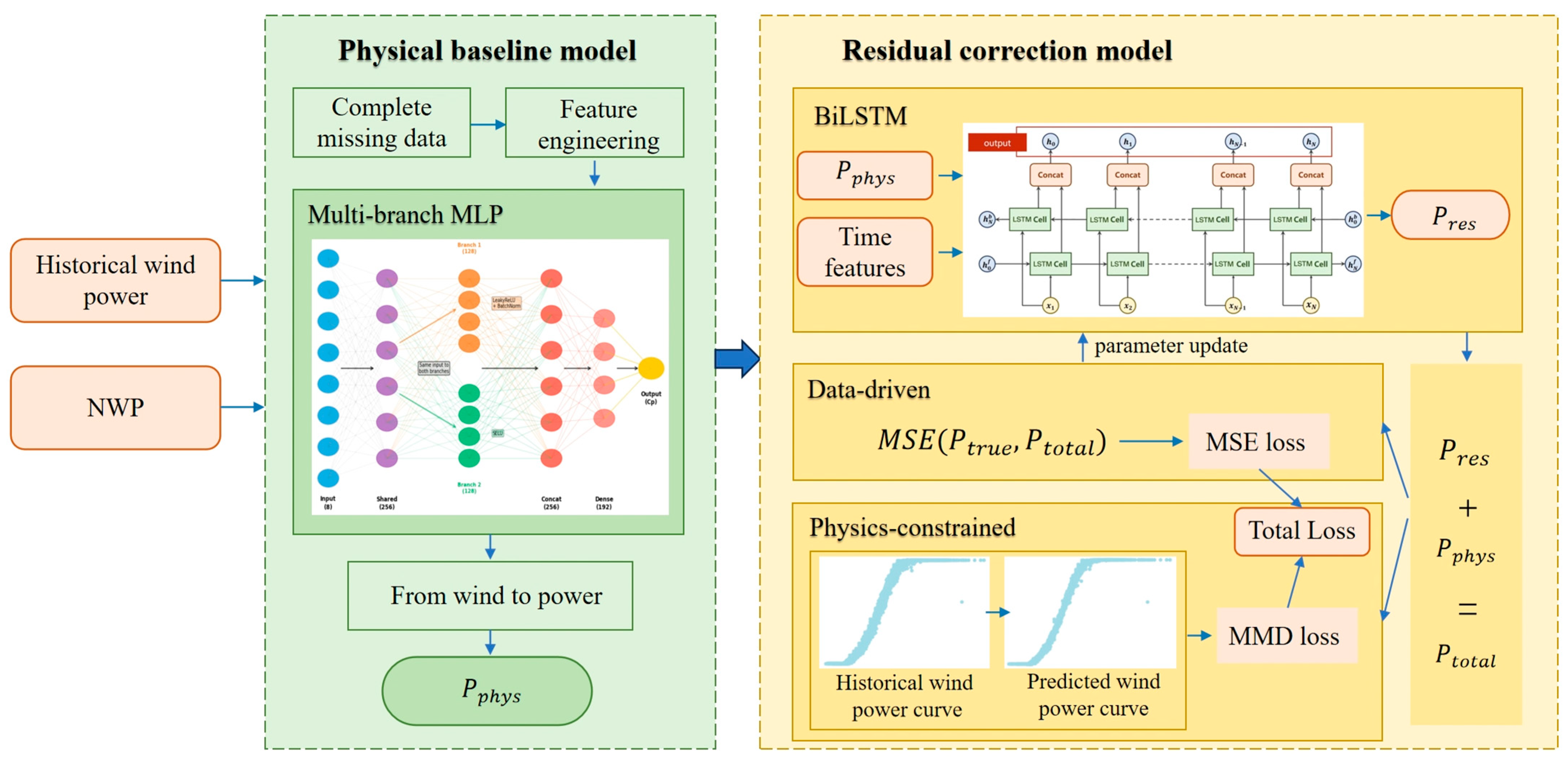
The structure of the proposed model is shown in Figure 1. To improve the accuracy and physical interpretability of wind power prediction, this paper designs and implements a physics-information guided hybrid deep learning prediction model. As shown in Figure 1, the model framework contains two core parts: the Physical baseline model and the Residual correction model, achieving high-precision prediction through a “baseline + correction” strategy.

First Stage: Physical Baseline Model. This stage aims to utilize known aerodynamic principles to construct a power prediction benchmark with clear physical meaning. The model first preprocesses the input historical wind power data and numerical weather prediction (NWP) data, including missing value imputation and feature engineering. Subsequently, a carefully designed multi-branch multilayer perceptron is used to learn the complex nonlinear relationships between multivariate meteorological features such as wind speed, temperature, and air pressure, and the wind energy utilization coefficient. Finally, the model combines the physical formula for wind turbine power output to convert the predicted Cp value into an initial physical power prediction value $P_{phys}$. This baseline model ensures that prediction results have a solid physical foundation.

Second Stage: Residual Correction Model. The goal of this stage is to compensate for the inherent bias of the physical baseline model and prediction errors caused by unmodeled dynamic factors (such as wake effects, equipment aging, etc.). The model employs bidirectional long short-term memory networks, which can effectively capture long-term dependencies and bidirectional contextual information in time series data. Its input features include not only the output $P_{phys}$ of the physical baseline model, but also incorporate refined temporal features and other relevant variables to accurately learn and predict the residual sequence $P_{res}$. The final total predicted power $P_{total}$ is obtained by adding the physical baseline prediction $P_{phys}$ and the residual prediction $P_{res}$.

$$P_{total}=P_{phys}+P_{res}$$

(1)

A major innovation of this model lies in the design of its hybrid loss function, which simultaneously integrates both data-driven and physical constraint paradigms. This model updates LSTM network parameters through a hybrid optimization method that combines standard loss functions with a probability distribution-based wind power curve. The core advantage of this design lies in enhancing the model’s noise robustness. Specifically, given that noisy data often manifests as perturbations to individual data points, this method utilizes the distribution information of the sample population during the training phase, enabling the model to reduce sensitivity to isolated outliers, effectively suppressing their destructive impact on the training process, ultimately achieving stronger anti-interference capability. The data-driven component employs mean square error loss, aiming to minimize point-to-point errors between the final predicted power $P_{total}$ and the true value $P_{true}$, ensuring prediction accuracy. The physical constraint component introduces Maximum Mean Discrepancy loss, measuring and minimizing the distribution difference between the predicted wind power curve (wind speed-power joint distribution) and the historical real wind power curve, thereby constraining the model to generate prediction results that conform to physical laws and have reasonable distributions, avoiding the generation of outliers.

In summary, the combination of this “baseline + correction” structure with the hybrid loss function enables the model not only to learn complex patterns in the data but also to follow basic physical principles, thus improving prediction accuracy while enhancing the model’s robustness and credibility.

2.2. Physical Baseline Model Based on Multi-Branch Multilayer Perceptrons

The kinetic energy of wind can be derived using classical mechanics formulas [44]. Through aerodynamic characteristic analysis, neglecting external damping and other influences, the mathematical model expression of wind turbines can be obtained as follows:

$$P_m=0.5\cdot \rho \cdot A\cdot v^3\cdot C_p$$

(2)

where $P_m$ is the mechanical power output of the wind turbine; $\rho$ is air density; $A$ is the rotor swept area; $v$ is wind speed; and $C_p$ is the power coefficient, a complex function affected by multiple factors such as tip speed ratio and pitch angle, directly reflecting the efficiency of wind turbines in capturing wind energy. This formula indicates that wind power is proportional to the cube of wind speed, and small changes in wind speed will cause significant fluctuations in power, making accurate wind speed prediction the core issue of wind power prediction.

Based on the above analysis, this paper proposes a novel wind power prediction approach: instead of attempting to accurately reconstruct three-dimensional spatiotemporal wind fields, we directly learn the power conversion characteristics of wind turbines under specific meteorological conditions from historical operational data. We treat the estimation of $C_p$ as a data-driven regression problem. Rather than attempting to analytically parse its complex physical composition, we utilize a deep neural network to directly learn the mapping relationship $f_{Cp}$ from easily obtainable meteorological and operational states to $C_p$:

$${\widehat{C}}_p=f_{Cp}\left({\mathbf{x}}_{Cp}\right)$$

(3)

where ${\widehat{C}}_p$ is the predicted value, and ${\mathbf{x}}_{Cp}$ is the input feature vector affecting $C_p$, which in this study includes ambient wind speed, ambient temperature, and engineering features derived from wind speed (such as wind speed squared, cubed, logarithm, etc.). The target value $C_p$ is back-calculated from actual power and wind speed in historical SCADA data through Formula (2).

To construct the mapping function $f_{Cp}$, we design a Multi-branch MLP. This network structure contains two parallel processing branches: one branch uses the LeakyReLU activation function, excelling at capturing sparse and nonlinear relationships in features; the other branch uses the self-normalizing activation function SELU, which helps achieve internal self-stabilization in the network, preventing gradient vanishing or explosion. The outputs of the two branches are concatenated and then fused through fully connected layers, ultimately outputting the predicted ${\widehat{C}}_p$ value. This structure can extract and integrate feature information from different perspectives, enhancing the model’s expressive capability.

After obtaining the predicted power coefficient ${\widehat{C}}_p$, the baseline predicted power $P_{phys}$ can be calculated through Formula (2):

$$P_{phys}={\displaystyle \frac{1}{2}}\rho A\left(\mathrm{clip}\left({\widehat{C}}_p,0,C_{pmax}\right)\right)v^3$$

(4)

where clip is a truncation function that limits the value of ${\widehat{C}}_p$ within the interval [0, $C_{pmax}$].

This baseline power $P_{phys}$ embodies the main aerodynamic performance of the wind turbine, providing a stable starting point with strong physical interpretability for subsequent residual correction.

2.3. Bidirectional LSTM Residual Correction Model

While the baseline model captures the main power conversion laws, its prediction errors still contain much dynamic information not captured by the model, such as short-term wind turbulence, lag effects of wind turbine control systems, and the impact of temperature on drivetrain efficiency. These residuals typically exhibit significant temporal correlations.

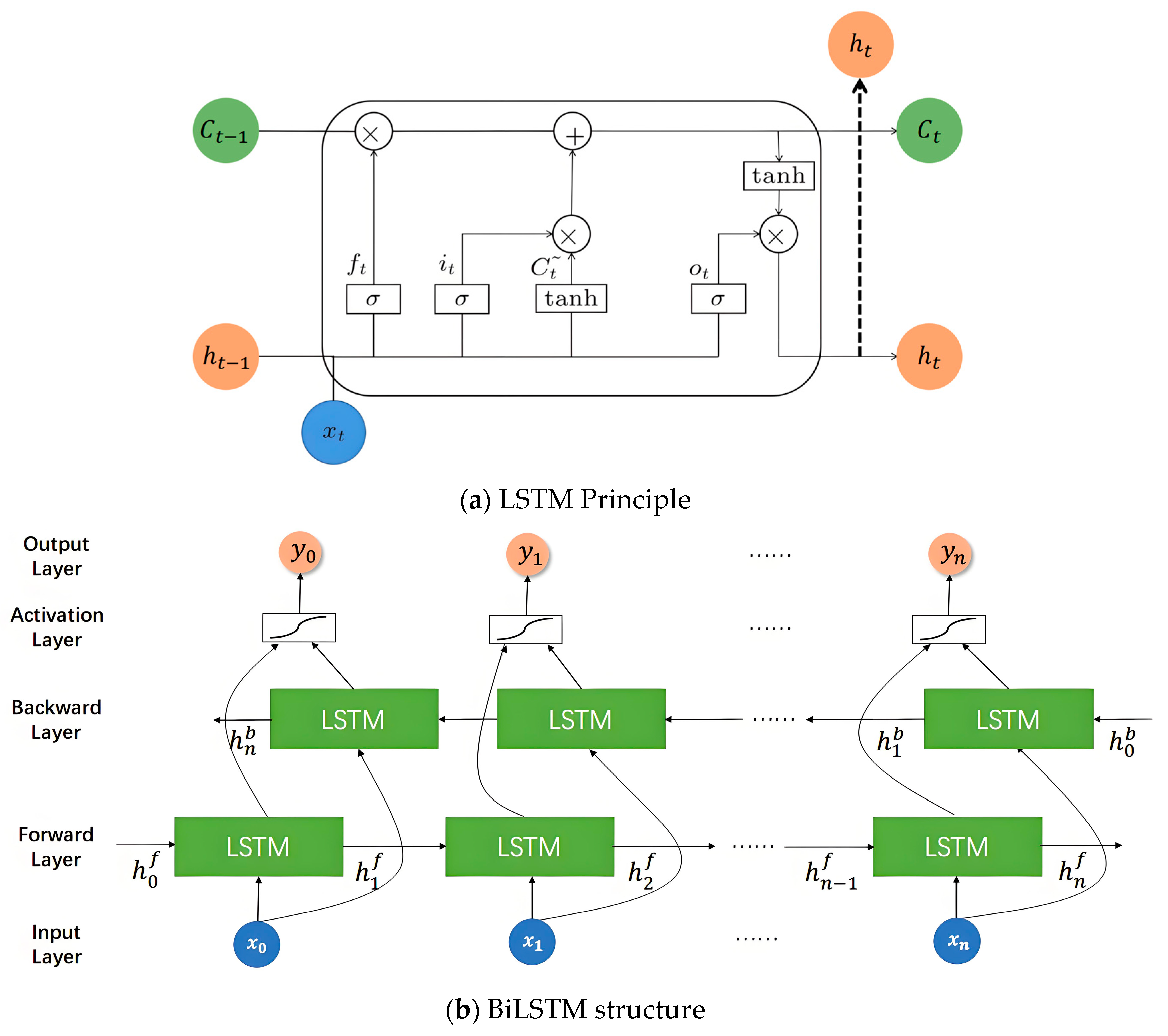
Long Short-Term Memory (LSTM) networks [45] are classic sequence models designed to overcome the gradient vanishing and explosion problems of traditional recurrent neural networks (RNN). Their core lies in the ingeniously designed gating units (including forget gate, input gate, and output gate), whose structure is shown in Figure 2a. This mechanism can regulate information flow in cell states, thereby achieving selective memory of sequence information. However, standard LSTM models can only utilize historical information unidirectionally. To more comprehensively exploit temporal dependencies in the data, this research employs bidirectional long short-term memory (BiLSTM) networks to model residual sequences, with the structure shown in Figure 2b. BiLSTM processes data in parallel through a forward LSTM layer and a backward LSTM layer, simultaneously integrating past and future contextual information at the current moment for prediction. This bidirectional information flow gives it advantages over unidirectional LSTM in capturing complex dynamic patterns, hence its selection as the modeling tool for residual sequences.

The BiLSTM used in the residual model has three input dimensions:

(1)

Batch size: the number of samples used in each training iteration, with a batch size of 32 used during training;

(2)

Time steps (lookback): the length of historical data used to predict current moment residuals, using 24 time steps here, representing the model processing 24 consecutive historical time points at once;

(3)

Feature dimensions: including environmental features (wind speed, temperature), baseline model predicted power, temporal cyclic features (hour, day, month, etc.), lag features (historical wind speed and baseline power), and rolling statistical features (mean and standard deviation of wind speed and baseline power), totaling 18 features.

The BiLSTM model in this paper contains 2 BiLSTM layers. The first BiLSTM layer has a hidden unit size of 64 and passes the complete sequence output to the next layer. The second BiLSTM layer has a hidden unit size of 32, used to capture deeper temporal dependencies. Following the BiLSTM layers is a fully connected layer with 32 neurons, used to extract higher-dimensional abstract representations from sequence features, further enhancing the model’s nonlinear fitting capability. The entire network also applies Dropout and BatchNormalization to prevent overfitting and stabilize the training process.

2.4. MMD Distribution Regularization Term

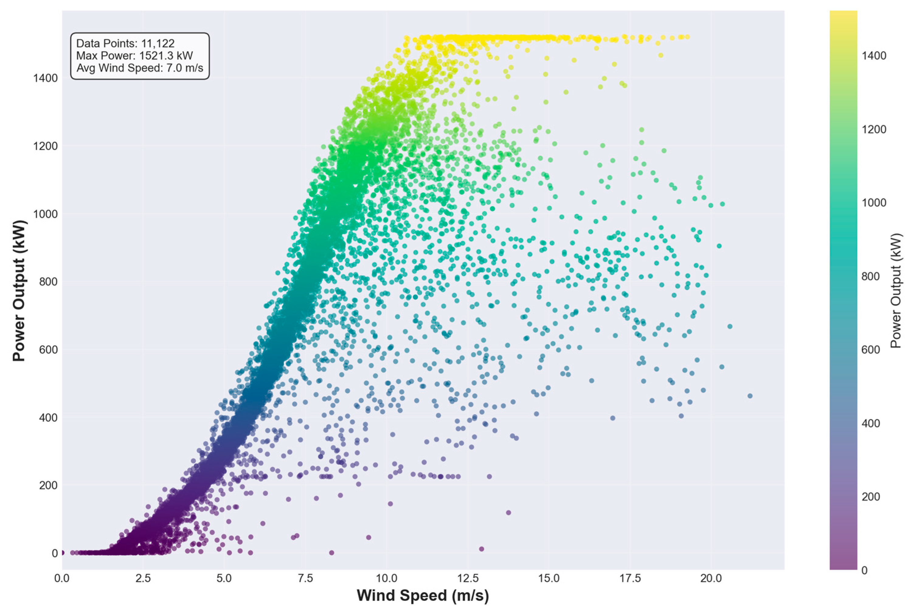
The Wind Power Curve is a core tool for describing the theoretical output power of wind turbine units at different wind speeds, intuitively reflecting the aerodynamic and mechanical performance of units converting wind energy into electrical energy. Ideally, this curve presents deterministic S-shaped characteristics, including key operational turning points such as cut-in wind speed, rated wind speed, and cut-out wind speed. However, in actual operating environments, the wind power generation process is not a deterministic system. Affected by multiple complex and difficult-to-fully-model factors such as air density fluctuations, wind shear, turbulence intensity, blade contamination, control system delays, and sensor measurement errors, the actual output power corresponding to a specific wind speed is not a fixed value but a random variable fluctuating within a range. Therefore, the actually observed wind power data points (wind speed-power pairs) do not strictly adhere to a single-valued curve but constitute a joint probability distribution, as shown in Figure 3.

Traditional deep learning models typically use the MSE loss function for training:

$$L_{MSE}={\displaystyle \frac{1}{N}}\sum _{i=1}^N (y_i-\widehat{y_i}{)}^2$$

(5)

where $y_i$ is the true value and $\widehat{y_i}$ is the predicted value. The MSE optimization objective is to minimize the point-to-point Euclidean distance between predicted and true values. While this method can effectively improve average prediction accuracy, it ignores the inherent structure of the wind speed-power joint distribution. This optimization approach may lead the model to produce “average correct but physically distorted” prediction results. For example, while the power value predicted at a specific wind speed may have a small error, the (wind speed, power) data pair it forms may deviate from high-density regions of the true data distribution, or even appear in physically impossible regions. This phenomenon weakens the model’s generalization ability and the physical credibility of prediction results.

To address this issue and guide the model to learn the inherent stochastic characteristics of the real wind power generation process, this research introduces a distribution regularization term based on Maximum Mean Discrepancy [46] into the model’s loss function. MMD is a non-parametric metric for measuring differences between two probability distributions. Its core idea is that if two distributions are the same, their expected values for any function should be equal in a sufficiently rich function space (Reproducing Kernel Hilbert Space, RKHS). MMD measures distribution differences by computing the supremum of these two expected values.

For two distributions $p$ and $q$, the square of their MMD can be expressed as:

$$MM{D}^2\left(p,\mathrm{q}\right)=\parallel {\mu }_p-{\mu }_q{\parallel }_{\mathcal{H}}^2$$

(6)

where ${\mu }_p$ and ${\mu }_q$ are the mean embeddings of distributions $p$ and $q$ in RKHS $\mathcal{H}$. If and only if $p=q$, then $MM{D}^2\left(p,q\right)=0$.

In our task, $p$ represents the wind speed-power joint distribution of historical real data $P_{hist}(v,P_{actual})$, and $q$ represents the wind speed-power joint distribution generated by the model in the current training batch $P_{pred}(v,P_{final})$. We use the Gaussian kernel (RBF kernel) function $k\left(x,y\right)=\exp \left(-{\displaystyle \frac{\left|\right|x-y|{|}^2}{2{\sigma }^2}}\right)$ to define the RKHS. The unbiased estimator of the square of MMD can be written as:

$$L_{MMD}={\displaystyle \frac{1}{m\left(m-1\right)}}\sum _{i\ne j}^m k\left(x_i,x_j\right)+{\displaystyle \frac{1}{n\left(n-1\right)}}\sum _{i\ne j}^n k\left(y_i,y_j\right)-{\displaystyle \frac{2}{mn}}\sum _{i=1}^m \sum _{j=1}^n k\left(x_i,y_j\right)$$

(7)

where $\{x_i{\}}_{i=1}^m$ are samples drawn from $p$ (historical real wind speed-power pairs), and $\{y_j{\}}_{j=1}^n$ are samples drawn from $q$ (wind speed-predicted power pairs from the current batch).

We add $L_{MMD}$ as a regularization term to the loss function, forming the final custom composite loss function:

$$L_{total}=L_{MSE}+\lambda \cdot L_{MMD}$$

(8)

where $L_{MSE}$ is used to ensure point prediction accuracy, $L_{MMD}$ is the MMD loss calculated according to Formula (7), used to ensure prediction distribution consistency. λ\lambda λ is a hyperparameter used to balance the importance of these two loss terms. By minimizing this hybrid loss function, the model optimizes residual prediction accuracy while also being “incentivized” to generate a wind speed-power relationship similar to the historical data distribution. This is equivalent to applying a “soft” physical constraint, making prediction results more likely to fall in high-probability, physically realistic regions, thereby effectively avoiding abnormal, outlier predictions and improving the model’s generalization ability and robustness.

2.5. Theoretical Foundations of the Proposed Framework

This section provides a theoretical analysis of the proposed two-stage physics-guided framework from the perspectives of mathematical optimization, statistical learning, and computational complexity. We demonstrate how the careful problem decomposition and physics embedding fundamentally simplify the learning task. The core advantages manifest in four aspects: improvement of the optimization landscape, effective decoupling of physics and data-driven components, mitigation of error propagation, and reduction in learning complexity. These theoretical analyses provide the mathematical foundation for the experimental validation in Section 3.

(1)

Fundamental Improvement of the Optimization Landscape

The optimization landscape—the surface formed by the loss function $\mathcal{L}\left(\theta \right)$ over the parameter space—directly governs the convergence behavior and stability of gradient-based learning algorithms. Traditional end-to-end approaches attempt to learn a single, highly complex function $f:\mathbf{x}\to P$ that directly maps input features to power output:

$$P=f\left(\mathbf{x}\right)+ϵ$$

(9)

where $ϵ$ represents complex error terms. In contrast, our framework (detailed in Section 2.1, Section 2.2, Section 2.3 and Section 2.4) decomposes the problem into two more tractable tasks. First, a data-driven model learns the function $g$ to predict the power coefficient:

$${\widehat{C}}_p=g\left(\mathbf{x}\right)$$

(10)

Subsequently, the known deterministic physics equation is applied to compute the baseline power prediction:

$$P_{\mathrm{base}}={\displaystyle \frac{1}{2}}\rho A{v}^3{\widehat{C}}_p$$

(11)

Although both features and targets are standardized during training (features via StandardScaler, $C_p$ via QuantileTransformer), predicting $C_p$ retains fundamental advantages over direct power prediction at the optimization level. These advantages manifest in the properties of the gradient space and the condition number of the loss landscape.

For direct power prediction, the gradient of the standardized loss function is:

$${\nabla }_{\theta }{\mathcal{L}}_p={\displaystyle \frac{\partial \mathcal{L}}{\partial \tilde{P}}}\cdot {\displaystyle \frac{\partial \tilde{P}}{\partial P}}\cdot {\displaystyle \frac{\partial P}{\partial \theta }}$$

(12)

where $\tilde{P}$ denotes standardized power. Since the original power $P={\displaystyle \frac{1}{2}}\rho A{v}^3{C}_p$ contains the $v^3$ term, this strong nonlinearity causes ${\displaystyle \frac{\partial P}{\partial \theta }}$ to vary dramatically across different wind speed regimes. For a typical 1.5 MW turbine, power ranges from 0 to 1500 kW with a variance of approximately:

$${\sigma }_P^2=\mathsf{{\rm E}}\left[\right(P-{\mu }_P{)}^2]\approx \mathrm{250,000}{ \mathrm{kW}}^2$$

(13)

When mapping such a wide range and highly nonlinear distribution of raw power values into standardized space, the StandardScaler must handle this extreme data distribution. In high wind speed regions, due to the rapid growth of $v^3$, data points are highly sparse in the original space. The standardization process leads to:

• Gradient vanishing or explosion at extreme power values
• Numerical instability during backpropagation
• Information loss in the standardization-destandardization cycle

In contrast, our approach predicts $C_p$ with gradients:

$${\nabla }_{\theta }{\mathcal{L}}_{C_p}={\displaystyle \frac{\partial \mathcal{L}}{\partial {\tilde{C}}_p}}\cdot {\displaystyle \frac{\partial {\tilde{C}}_p}{\partial C_p}}\cdot {\displaystyle \frac{\partial C_p}{\partial \theta }}$$

(14)

The key advantage is that $C_p$ is physically bounded by the Betz limit within $[0, 0.59]$, representing a bounded physical quantity with relatively uniform distribution. Its variance is merely:

$${\sigma }_{C_p}^2=\mathsf{{\rm E}}\left[\right(C_p-{\mu }_{C_p}{)}^2]\approx 0.015$$

(15)

This represents a variance reduction factor of approximately $10^7$. The QuantileTransformer mapping is significantly more stable on such bounded, regular distributions. More importantly, ${\displaystyle \frac{\partial C_p}{\partial \theta }}$ does not contain the strong nonlinearity of $v^3$, ensuring that gradients maintain a superior condition number throughout training.

From an optimization theory perspective, for loss functions with $L$-Lipschitz gradients, the convergence rate of gradient descent satisfies:

$$\mathcal{L}\left({\theta }_t\right)-\mathcal{L}\left({\theta }^{*}\right)\le {\displaystyle \frac{L\parallel {\theta }_0-{\theta }^{*}{\parallel }^2}{2t}}$$

(16)

where $L$ is the Lipschitz constant (upper bound on gradient variation), and ${\theta }^{*}$ denotes optimal parameters. For strongly convex functions, the rate improves to:

$$\mathcal{L}\left({\theta }_{t+1}\right)-\mathcal{L}\left({\theta }^{*}\right)\le {\left(1-{\displaystyle \frac{\mu }{L}}\right)}^t\left[\mathcal{L}\left({\theta }_0\right)-\mathcal{L}\left({\theta }^{*}\right)\right]$$

(17)

where $\mu$ is the strong convexity parameter, and the condition number $\kappa =L/\mu$ directly affects convergence speed. While neural network losses are non-convex, local convexity and smoothness properties still apply.

Due to the boundedness ($\mid C_p\mid \le 0.59$) and relative smoothness (absence of $v^3$ term) of $C_p$, the loss landscape for predicting $C_p$ exhibits the following to enable faster convergence:

• Smaller Lipschitz constant: $L_{C_p}\ll L_P$
• Better condition number: ${\kappa }_{C_P}<{\kappa }_P$

(2)

Effective Decoupling of Known Physics and Unknown Dynamics

In end-to-end models, the neural network is forced to simultaneously learn:

(a)

Governing physical laws: the cubic relationship between power and wind speed $P\propto v^3$

(b)

The complex power coefficient function $C_p(\lambda ,\beta )$ (dependent on tip-speed ratio and pitch angle)

(c)

Various stochastic deviations and unmodeled dynamics $ϵ$

This represents an inefficient entanglement of learning tasks. Our framework explicitly encodes the highly nonlinear $v^3$ relationship into the deterministic physics equation, relieving the neural network of the burden to “re-learn” this fundamental physical principle. Consequently, the data-driven model $g\left(\mathbf{x}\right)$ can dedicate its full capacity to the more nuanced task: precisely learning how the turbine’s aerodynamic efficiency ($C_p$) varies dynamically across different operating conditions and environmental factors.

This decomposition effectively factorizes the problem into the following:

$$P=\underset{\mathrm{Physical} \mathrm{law}}{\underbrace{{\displaystyle \frac{1}{2}}\rho A{v}^3}}\cdot \underset{\mathrm{Data}\text{-}\mathrm{driven}}{\underbrace{{\widehat{C}}_p}}+\underset{\mathrm{Residual} \mathrm{correction}}{\underbrace{\widehat{ϵ}}}$$

(18)

This presents a smoother, better-behaved function $g$ for the neural network to approximate, thereby enhancing learning efficiency and accuracy.

From the perspective of function approximation theory, based on generalizations of the universal approximation theorem, approximation complexity relates to the variation and degree of nonlinearity of the function. Let ${\mathcal{F}}_{\mathrm{direct}}$ denote the function class for direct power prediction and ${\mathcal{F}}_{C_p}$ for $C_p$ prediction. Their Rademacher complexity (a measure of function class richness) satisfies:

$${\mathcal{R}}_n\left({\mathcal{F}}_{\mathrm{d}\mathrm{i}\mathrm{r}\mathrm{e}\mathrm{c}\mathrm{t}}\right)=\mathcal{O}\left({\displaystyle \frac{B_P\sqrt{d_{\mathrm{e}\mathrm{f}\mathrm{f}}}}{\sqrt{n}}}\right)$$

(19)

$${\mathcal{R}}_n\left({\mathcal{F}}_{C_p}\right)=\mathcal{O}\left({\displaystyle \frac{B_{C_p}\sqrt{d_{\mathrm{e}\mathrm{f}\mathrm{f}}^{\prime }}}{\sqrt{n}}}\right)$$

(20)

where $B_P$ and $B_{C_p}$ are upper bounds of the function classes, $d_{\mathrm{e}\mathrm{f}\mathrm{f}}$ and $d_{\mathrm{e}\mathrm{f}\mathrm{f}}^{\prime }$ are effective dimensions, and $n$ is the sample size. Due to:

• $C_p\in [0, 0.59]$ being bounded, thus $B_{C_p}\ll B_P$ (power range $[0, 1500]$)
• $C_p$ varying more smoothly with respect to input features (lacking the strong nonlinearity of the $v^3$ term)
• Effective dimension $d_{\mathrm{eff}}^{\prime }<d_{\mathrm{eff}}$ (task decomposition reduces complexity)

Therefore:

$${\mathcal{R}}_n\left({\mathcal{F}}_{C_p}\right)\ll {\mathcal{R}}_n\left({\mathcal{F}}_{\mathrm{d}\mathrm{i}\mathrm{r}\mathrm{e}\mathrm{c}\mathrm{t}}\right)$$

(21)

According to statistical learning theory, generalization error bounds are proportional to Rademacher complexity. Smaller Rademacher complexity implies:

$${\mathrm{Generalization} \mathrm{error}}_{C_p}\le {\mathrm{Empirical} \mathrm{error}}_{C_p}+\mathcal{O}\left({\mathcal{R}}_n\right({\mathcal{F}}_{C_p}\left)\right)\ll {\mathrm{Generalization} \mathrm{error}}_{\mathrm{direct}}$$

This theoretically guarantees superior generalization performance and reduced overfitting risk.

(3)

Mitigation of Error Propagation

While the cubic relationship between wind speed and power is physically accurate, it also acts as a significant amplifier of input measurement errors. Let the wind speed measurement error be $\Delta v$; then the power error is:

$$\Delta P_{\mathrm{d}\mathrm{i}\mathrm{r}\mathrm{e}\mathrm{c}\mathrm{t}}={\displaystyle \frac{\partial P}{\partial v}}\Delta v+{\displaystyle \frac{1}{2}}{\displaystyle \frac{{\partial }^{2}P}{\partial v^2}}(\Delta v{)}^2+\cdots ={\displaystyle \frac{3}{2}}\rho A{v}^2{C}_p\Delta v+\mathcal{O}(\left(\Delta v{)}^2\right)$$

(22)

In other words, $\Delta P\propto v^2\Delta v$. Under typical high wind conditions (e.g., $v=15$ m/s), even a 5% wind speed measurement error ($\Delta v=0.75$ m/s) leads to approximately the following:

$${\displaystyle \frac{\Delta P}{P}}\approx 3{\displaystyle \frac{\Delta v}{v}}=3\times 5\mathrm{\%}=15\mathrm{\%}$$

(23)

The power error can be further amplified to 34% under the cubic relationship.

In end-to-end approaches, the model must learn in this cubically amplified noise environment, resulting in the following:

• Training instability
• High sensitivity to input noise
• Poor generalization capability

In our approach, the neural network learns:

$${\widehat{C}}_p=g\left(\mathbf{x}\right)+{\delta }_{C_p}$$

(24)

Although wind speed errors will ultimately propagate through $P={\displaystyle \frac{1}{2}}\rho A{v}^3{\widehat{C}}_p$ to the final power prediction, the learning process of $C_p$ itself is decoupled from the $v^3$ amplification effect. The model learns to map inputs to a stable $C_p$ target, which is far less sensitive to cubic nonlinearity than direct power prediction. The final power error can be decomposed as follows:

$$\Delta P={\displaystyle \frac{1}{2}}\rho A{v}^3{\delta }_{C_p}+{\displaystyle \frac{3}{2}}\rho A{v}^2{\widehat{C}}_p\Delta v$$

(25)

The key distinction is that ${\delta }_{C_p}$ is learned on a stable, bounded target, making it inherently smaller and more robust to input noise. While the second term remains subject to the cubic relationship, this is an unavoidable physical reality rather than additional instability introduced by the learning process.

This architectural choice makes the training process of the data-driven component more robust and less sensitive to the inherent noise and uncertainty common in real wind speed measurements, ultimately producing more accurate and stable predictions.

3. Results

3.1. Data Analysis

The experiments in this study are conducted on a publicly available dataset to ensure the transparency and reproducibility of our results. This research selects the Spatial Dynamic Wind Power Forecasting (SDWPF) dataset constructed based on actual wind farm data from Longyuan Power Group Co., Ltd. (Beijing, China) for experiments [47]. The dataset provides output power, wind speed, ambient temperature, and other characteristics for 134 wind turbines, sampled every 10 min from January 2020 to December 2021. To ensure data quality, we first preprocessed the dataset by extracting coherent segments with minimal missing values from multiple turbines.

To rigorously evaluate the effectiveness and generalizability of our proposed method, experiments were conducted across several different turbines. In the main body of this paper, we present a detailed analysis using turbine 112 as a representative case, for which the processed dataset contains 16,109 sample points. The corresponding results for other turbines, which demonstrate consistent performance, are provided in Appendix B. For all experiments, each turbine’s dataset was divided chronologically into a training set (70%), a validation set (20%), and a test set (10%). This chronological split ensures that the model’s generalization capability is evaluated fairly, without any information leakage from the future.

3.2. Evaluation Metrics

To comprehensively analyze the model’s prediction effects and evaluate model performance, this paper employs Mean Square Error (MSE), Mean Absolute Error (MAE), Root Mean Square Error (RMSE), and coefficient of determination (R²) to evaluate the model’s prediction accuracy. The corresponding calculation formulas are as follows:

$$MSE={\displaystyle \frac{1}{N}}\sqrt{\sum _{i=1}^N {\left(X_i-Y_i\right)}^2}$$

(26)

$$MAE={\displaystyle \frac{1}{N}}\sum _{i=1}^N \left|\begin{array}{c}{X}_i-Y_i\end{array}\right|$$

(27)

$$RMSE=\sqrt{{\displaystyle \frac{1}{N}}\sum _{i=1}^N {\left(X_i-Y_i\right)}^2}$$

(28)

$$\sum _{i=1}^N {\left(X_i-Y_i\right)}^2{R}^2=1-{\displaystyle \frac{\sum _{i=1}^N {\left(Y_i-\widehat{Y}\right)}^2}{\sum _{i=1}^N {\left(Y_i-\widehat{Y}\right)}^2}}$$

(29)

where $N$ is the total number of samples, $X_i$ is the predicted value of the $i$-th data point, $Y_i$ is the true value of the $i$-th data point, and $\widehat{Y}$ is the average value of the samples.

3.3. Experimental Setup and Parameter Settings

The training process is divided into two distinct stages. In the first stage, the baseline model is trained to predict the power coefficient (Cp). For this non-sequential task, input features were scaled using StandardScaler, and the target variable (Cp) was transformed using QuantileTransformer to handle its non-Gaussian distribution, which helps stabilize training and allows the model to better learn the underlying patterns. In the second stage, the residual correction model is trained. This model takes sequence data as input, with a lookback window of 24 time steps (i.e., 4 h of historical data), which was chosen as a balance between capturing relevant short-term dynamics (e.g., turbulence effects, control system inertia) and maintaining computational efficiency. The input features for this stage were also normalized using StandardScaler. To optimize the training process and prevent overfitting, we employed several callback functions. ModelCheckpoint was used to save the model with the best performance on the validation set. ReduceLROnPlateau was implemented to dynamically adjust the learning rate when the validation loss plateaued. For the baseline model, EarlyStopping was also used to halt training if no improvement was observed over a set number of epochs. The specific hyperparameters for both models are summarized in

Table 1. Hyperparameter Settings for the Proposed Models.

Paramter	Stage 1: Baseline (Cp) Model	Stage 2: Residual (BiLSTM) Model
Model Type	Multi-branch Multilayer Perceptron (MLP)	2-layer Bidirectional LSTM
Architecture Details	Dense (256, LeakyReLU) Branch A: Dense (128, LeakyReLU) Branch B: Dense (128, SELU) Concatenate → Dense (192, LeakyReLU)	BiLSTM (64, tanh, return_seq = True) BiLSTM (32, tanh) Dense (32, LeakyReLU)
Common Layers	BatchNormalization after each Dense layer	BatchNormalization and Dropout
Optimizer	Adam	Adam
Learning Rate	Initial: 0.0005, with ReduceLROnPlateau (patience = 10, factor=0.5)	Initial: 0.001, with ReduceLROnPlateau (patience = 15, factor = 0.5)
Batch Size	64	32
Max Epochs	200	200
Callbacks	EarlyStopping (patience = 30), ReduceLROnPlateau, ModelCheckpoint	ReduceLROnPlateau, ModelCheckpoint
Dropout Rate	0.3, 0.4	0.4 (for Dense layers), 0.1 (recurrent dropout)
Regularization	L2 kernel regularizer (1 × 10−4)	Not applied
Sequence Length	(Non-sequential model)	24
MMD Loss Weight (λ)	-	0.02
MMD Kernel Sigma (σ)	-	0.5

and

Table 2. Detailed Description of Model Input Features.

Feature Category	Description	Model Used
Original Features	Average wind speed (m/s)	Both models
	Ambient temperature (°C)	Both models
Derived Features	Wind speed squared	Baseline model
	Wind speed cubed	Baseline model
	Logarithmic transformation of wind speed	Baseline model
	Power-to-wind speed ratio	Baseline model
	Wind speed-to-power ratio	Baseline model
	Wind speed binning (6 intervals)	Baseline model
	Baseline predicted power	Residual model
Time Features	Hourly periodic encoding	Residual model
	Daily periodic encoding	Residual model
	Monthly periodic encoding	Residual model
	Day of the week	Residual model
Lag Features	Wind speed lags (1–3 steps)	Residual model
	Baseline power lags (1–2 steps)	Residual model
Statistical Features	6-step rolling mean of wind speed	Residual model
	6-step rolling standard deviation of wind speed	Residual model
	6-step rolling mean of baseline power	Residual model

.

To ensure a realistic and rigorous evaluation that simulates real-world deployment, our proposed framework was evaluated on the test set using a step-by-step iterative forecasting strategy. This method strictly avoids any future information leakage. Specifically, for each time step t in the test set, after predicting the power value, this prediction is used to dynamically update the feature set (e.g., lag and rolling statistical features) required for making the prediction at the subsequent time step t + 1. This autoregressive evaluation approach provides a true test of a model’s generalization capability in a live operational scenario, making the comparison far more stringent than a simple one-shot prediction where all future input features are assumed to be known. For a comprehensive, step-by-step breakdown of the entire training and evaluation workflow, please refer to the pseudocode in Appendix A.

To establish a strong set of benchmarks, all comparison models (BiLSTM, iTransformer, PatchTST, TimesNet, VMD-Transformer, and VMD-BiLSTM) were configured to ensure a fair and consistent evaluation. They were all trained as end-to-end models, directly mapping historical data to future power output.

Input Features: A comprehensive set of 18 standard time-series features was engineered and used for all comparison models. This set includes:

• Raw Features: wind_speed, temperature.
• Physics-informed Features: ws_squared, ws_cubed.
• Temporal Features: hour_sin, hour_cos, dow_sin (day of week), dow_cos.
• Lag Features: Lagged values for 1, 2, and 3 previous time steps for both wind_speed and power.
• Rolling Statistics: 6-step rolling mean and standard deviation for both wind_speed and power.

Training Process: For all comparison models, the input features were normalized using StandardScaler. The models were trained to predict the next time step’s power value using a sequence length (lookback window) of 24 steps. The training process for each model utilized an Adam optimizer with an initial learning rate of 0.001, a batch size of 32, and was run for a maximum of 100 epochs. To prevent overfitting and optimize training, we employed EarlyStopping with a patience of 20 epochs and ReduceLROnPlateau with a patience of 10 epochs.

3.4. Experimental Results Analysis

• Comparative Experiments

To eliminate the influence of randomness in single training results on evaluation outcomes, this research conducted 10 independent training sessions for each model, and on this basis, removed the maximum and minimum values for each evaluation metric. Finally, we calculated the average of the remaining 8 training sessions as a more robust evaluation metric.

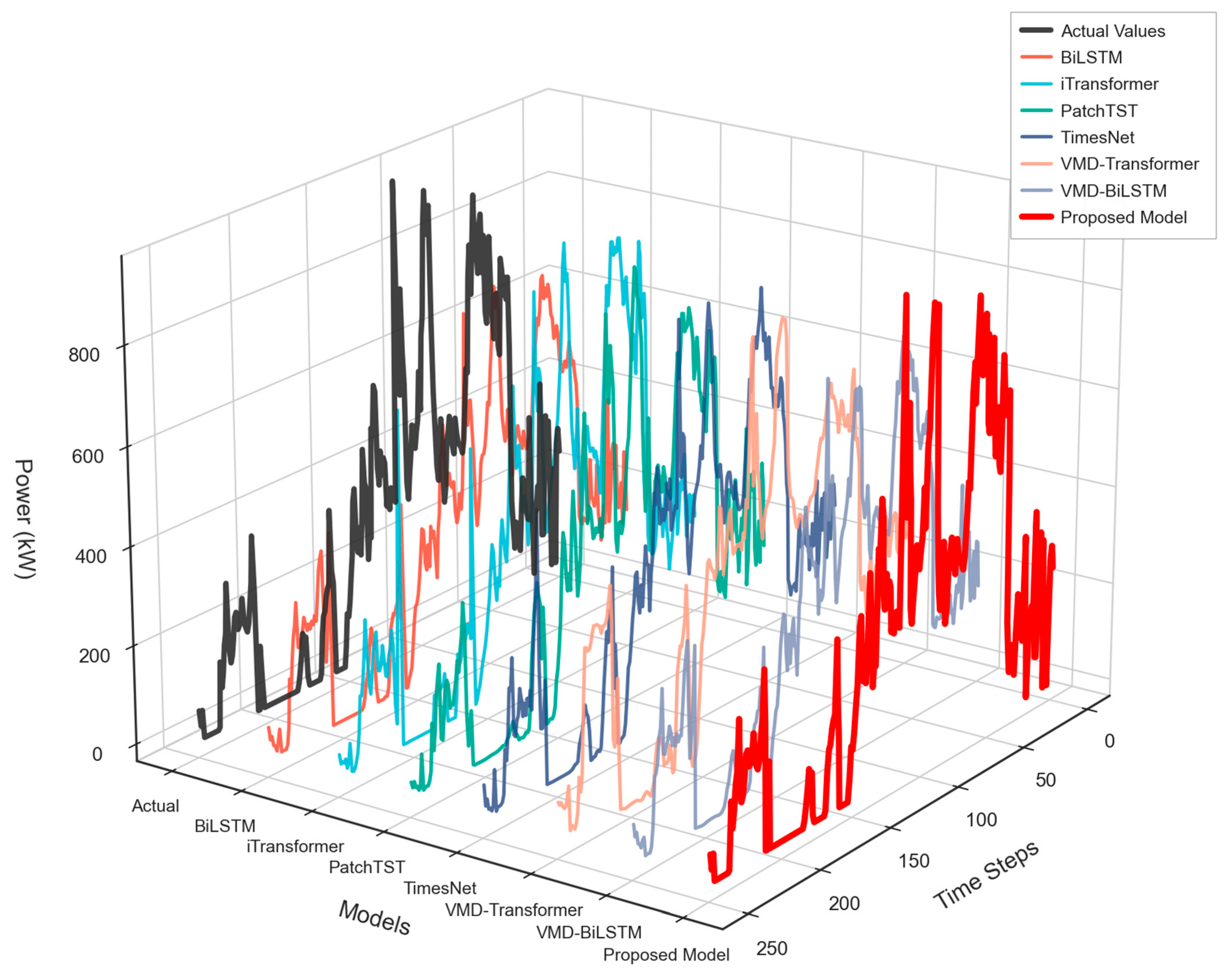
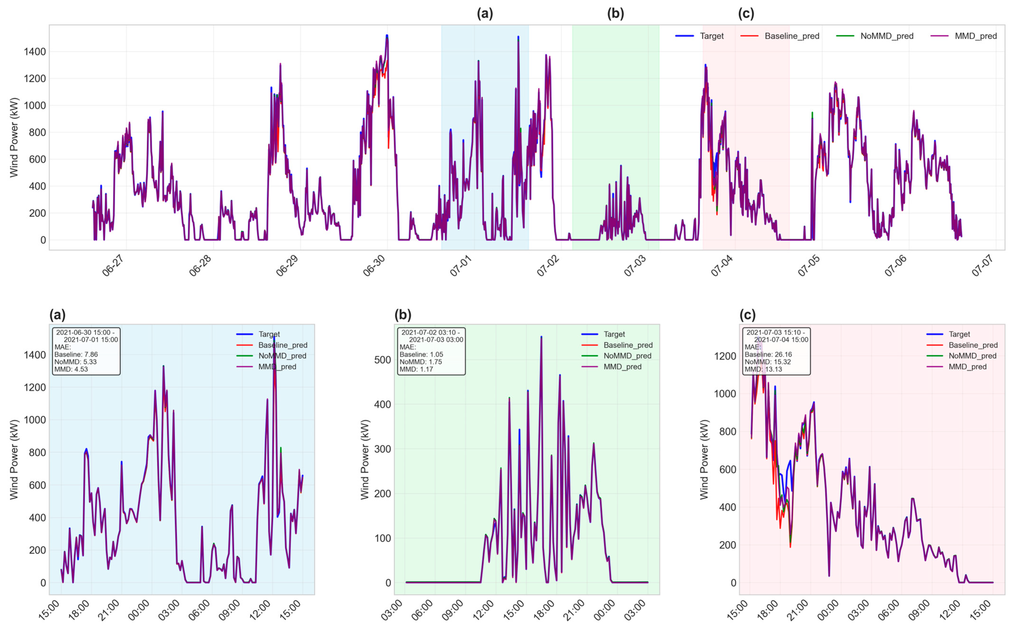
This paper introduces several classic models, including BiLSTM, iTransformer, PatchTST, TimesNet, VMD-Transformer, and VMD-BiLSTM, for comparative experiments. Taking turbine 112 data as an example, the power prediction comparison is shown in Figure 4. The experimental result metrics are shown in

Table 3. Multi-Model Experimental Result Metrics.

Model	MAE (kW)	MSE (kW2)	RMSE (kW)	R2
Proposed Model	5.66	293.61	17.14	0.9976
VMD-BiLSTM	56.33	7807.21	88.36	0.9358
TimesNet	56.26	7861.13	88.66	0.9354
PatchTST	59.41	8496.27	92.18	0.9302
BiLSTM	59.02	8540.82	92.42	0.9298
iTransformer	62.24	9934.71	99.67	0.9184
VMD-Transformer	96.23	21,251.65	145.78	0.8254

Note: The bolded values in this table indicate the best performance metrics among all models.

.

The results demonstrate that the physics-constrained deep learning method proposed in this paper achieves significantly superior performance to comparison methods on all metrics. Compared to the baseline BiLSTM, MAE decreased substantially from 59.02 kW to 5.66 kW (90.4% reduction), RMSE decreased from 92.42 kW to 17.14 kW (81.5% reduction), and R² improved from 0.9298 to 0.9976 (6.78 percentage points improvement). Even compared to the second-best performing VMD-BiLSTM, our method’s MAE still decreased by 90.0% (from 56.33 kW to 5.66 kW).

The substantial, order-of-magnitude performance improvement of our proposed model over strong baselines can be attributed to the synergistic effect of its unique design, which deeply integrates domain knowledge. The key reasons are threefold:

First, the physics-guided two-stage framework decomposes the complex prediction task. By first modeling the power coefficient (Cp), a physically meaningful quantity, the baseline model provides a robust and interpretable foundation that already captures the core aerodynamics, which is a significant structural advantage over end-to-end models.

Second, our model leverages highly specialized, domain-specific feature engineering for the Cp prediction stage. Features such as power_ws_ratio and wind_speed_bin are derived directly from wind energy principles and allow the model to learn the turbine’s operational characteristics with much higher fidelity than the more generic features used for the comparison models.

Third, the MMD distribution constraint acts as a final refinement layer, ensuring the model’s predictions are not only accurate on average but also conform to the physical plausibility reflected in the historical wind speed-power joint distribution. It is the combination of these three elements—a superior framework, richer features, and physical constraints—that results in the observed significant leap in performance.

The hybrid model proposed in this paper achieves an order of magnitude performance improvement compared to all comparison methods (MAE reduced from 56.26–96.23 kW to 5.66 kW, R² improved from 0.8254–0.9358 to 0.9976). This improvement is primarily attributed to the following key designs: First, the model adopts a modeling strategy combining physical mechanisms with data-driven approaches, decomposing power prediction into theoretical power calculation conforming to aerodynamic principles and residual compensation through introducing the wind energy utilization coefficient (Cp), avoiding the “black box” nature of purely data-driven methods. Second, feature engineering designed specifically for wind power characteristics fully considers the cubic relationship between wind speed and power (ws_cubed), dynamic temporal features (lag and rolling statistics), and segmented modeling of different operating conditions, effectively capturing the nonlinear dynamic characteristics of wind power systems. Third, the Maximum Mean Discrepancy (MMD) constraint ensures consistency between the predicted wind speed-power joint distribution and historical data, enhancing the model’s generalization ability and physical reasonableness. The synergistic effect of these innovations demonstrates that effectively integrating domain knowledge within deep learning frameworks can significantly improve the accuracy and reliability of wind power prediction.

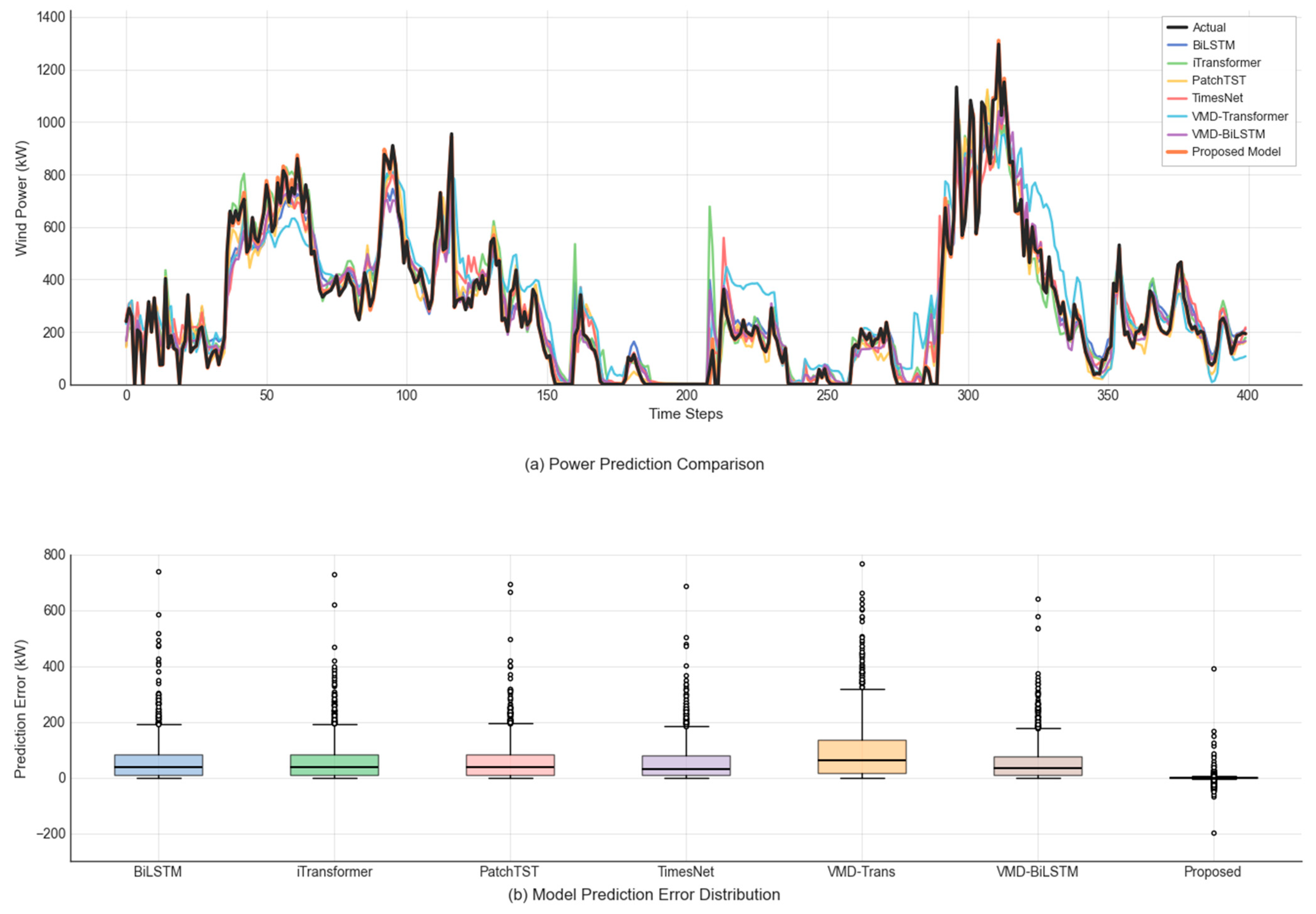
Figure 5 presents the prediction error distribution of different models on the test set. Our method’s error distribution is highly concentrated around zero, with a median error of 0.0 kW, a mean error of only −0.4 kW, a standard deviation of only 17.1 kW, the box plot compressed almost to a line, and almost no outliers, demonstrating extremely high prediction accuracy and stability. In contrast, all comparison methods’ error distributions deviate significantly from zero, showing notable positive bias characteristics, with median errors ranging from 31.6 kW to 62.4 kW, mean errors from 56.3 kW to 96.2 kW, standard deviations from 68.1 kW to 109.5 kW, not only large in error magnitude but also dispersed in distribution, with numerous outliers exceeding 200 kW.

2.

Performance Analysis by Power Segments

Taking turbine 112 as an example,

Table 4. Prediction Performance Analysis by Power Segments.

Power Segment	Number of Samples	MAE (kW)	RMSE (kW)
Low Power (<500 kW)	1017	2.52	10.37
Medium Power (500–1000 kW)	334	14.14	33.57
High Power (>1000 kW)	86	9.92	14.46

shows the prediction performance of our method across different power segments.

Table 4 demonstrates the performance differences of our method across different power segments, reflecting the challenging characteristics of wind power prediction under different operating conditions. In the low power segment, the model exhibits optimal prediction accuracy with an MAE of only 2.52 kW and an RMSE of 10.37 kW. The medium power segment presents the greatest prediction challenge, with MAE rising to 14.14 kW and RMSE reaching 33.57 kW. This power segment is in the nonlinear transition region where the turbine transitions from partial load to rated power, where power is extremely sensitive to wind speed changes, and small wind speed prediction deviations can lead to large power errors. Combined with relatively fewer samples in this segment, modeling difficulty is further increased. The high power segment, though having the fewest samples, shows MAE decreasing to 9.92 kW and RMSE of 14.46 kW, with prediction performance superior to the medium power segment. This is because after the turbine approaches or reaches rated power, power output tends to stabilize, and pitch control reduces power-wind speed sensitivity.

3.

Ablation Study

To verify the contribution of each module component, ablation experiments were conducted. Model 1 represents the complete model proposed in this research, Model 2 removes the MMD constraint, Model 3 uses only baseline power, and Model 4 uses only data-driven approaches. The results are shown in

Table 5. Ablation Experiment Results.

Configuration	MAE (kW)	RMSE (kW)	R2	Improvement (%)
Model 1	5.66	17.14	0.9976	89.5%
Model 2	5.67	18.72	0.9971	88.7%
Model 3	10.30	33.61	0.9907	77.6%
Model 4	59.02	92.42	0.9298	-

and Figure 6.

The results indicate that: the baseline power contributes most significantly, validating the importance of the physical model; the residual learning mechanism provides 11.1% performance improvement, effectively capturing complex nonlinear deviation patterns; the MMD constraint provides approximately 1% performance improvement, playing an important fine-tuning role in model stability, ensuring prediction distribution consistency with historical data, and improving generalization.

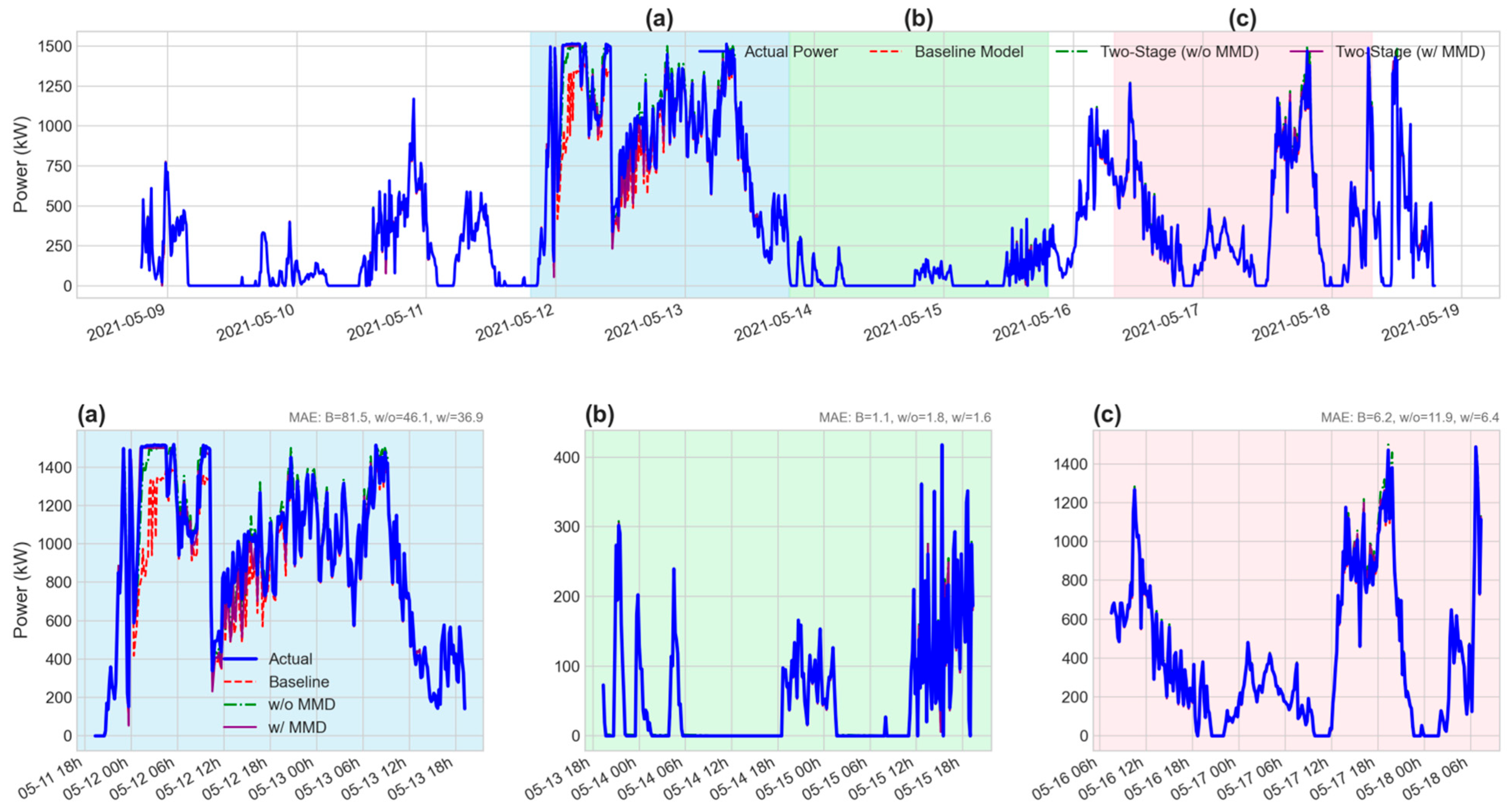
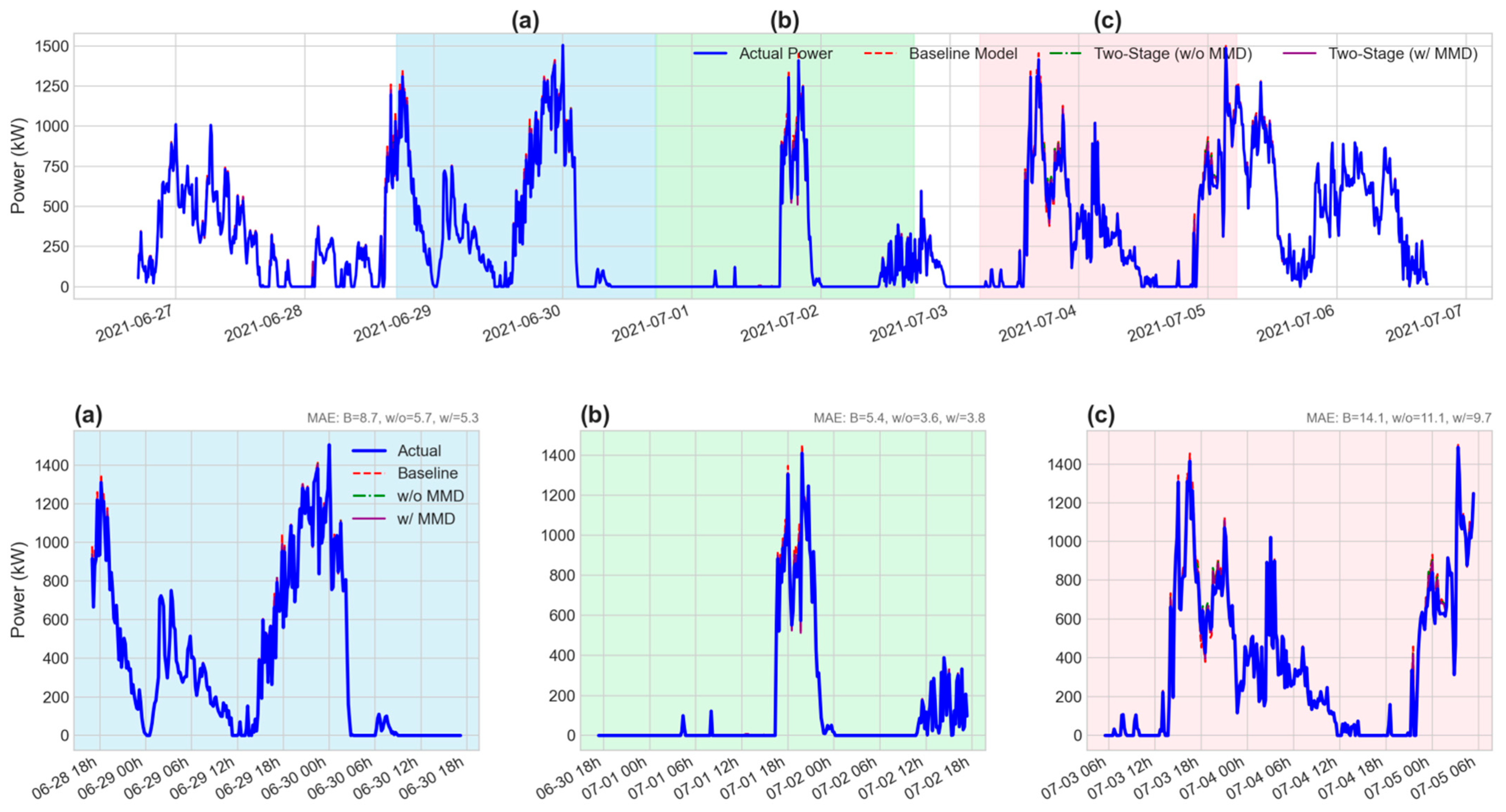
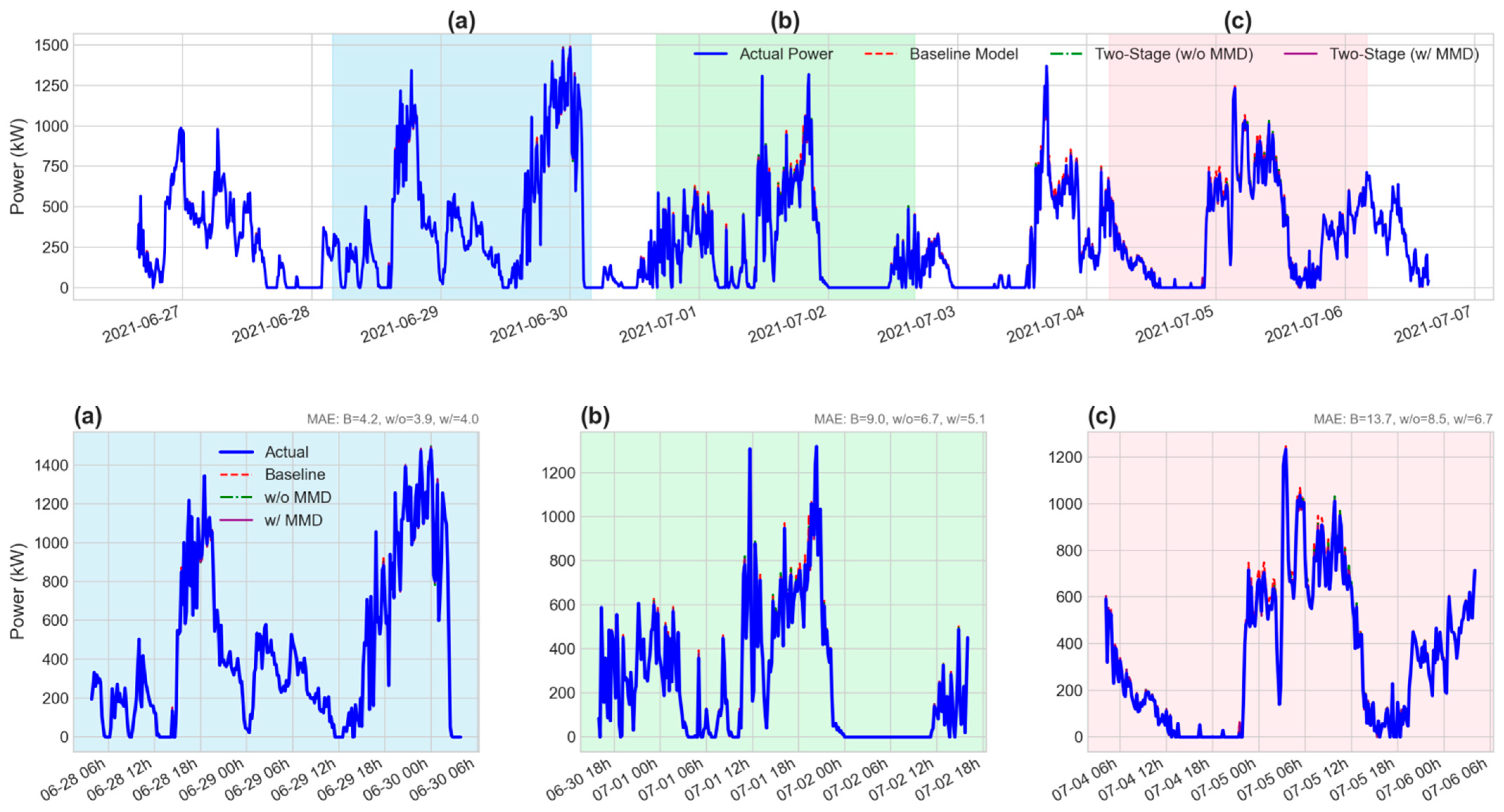
The results presented in Table 3 and Figure 5 clearly demonstrate the superiority of our proposed model on Turbine 112. To ensure these findings are not specific to a single unit and to validate the generalizability of our approach, we replicated the entire experiment on three other turbines. The detailed results of this generalization study, which show a similar pattern of outperformance, are presented in Appendix B.

4.

Convergence and Efficiency Analysis

To quantitatively evaluate the advantages of our proposed physics-guided paradigm in terms of training efficiency and generalization performance, we designed a rigorous comparative experiment. We compare our model (the Cp model) against a conventional model that employs the same BiLSTM core but directly predicts power in an end-to-end fashion. To ensure a fair comparison, both models maintain identical network depth, parameter scale, and training hyperparameters.

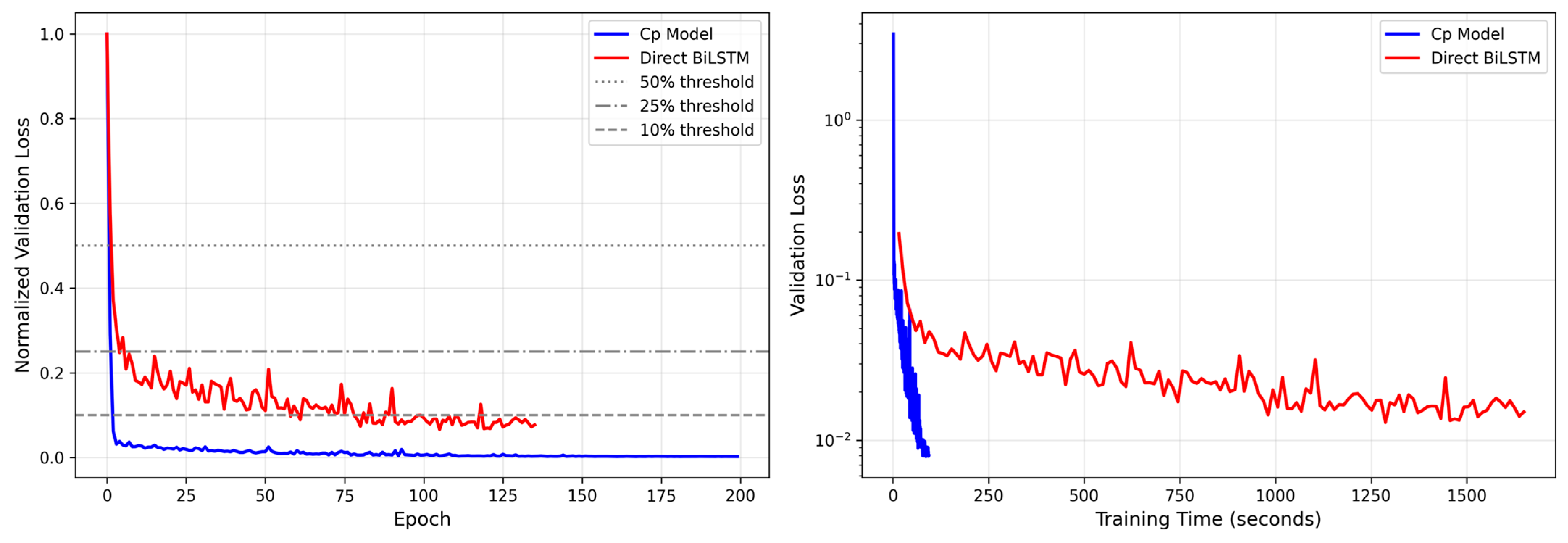
The experimental results, depicted in Figure 7, clearly illustrate the stark differences in the convergence process between the two paradigms.

First, our model demonstrates a decisive advantage in convergence speed. As shown by the normalized loss curve on the left, our Cp model (blue line) rapidly converges to a stable, low-error plateau within the first 20 epochs. In contrast, the training process of the direct prediction model (red line) is not only significantly slower but is also fraught with sharp oscillations, never consistently dropping below the 10% loss threshold and indicating a more complex and unstable optimization landscape. The wall-clock time plot on the right further substantiates this finding: our model achieves its optimal performance in approximately 100 s, whereas the direct model requires over 1600 s to complete its training, resulting in a more than 16-fold improvement in training efficiency.

Second, our model also excels in terms of final accuracy and generalization ability. As seen in the right plot of Figure 7, the final validation loss to which our model converges (settling just below 0.01) is substantially lower and more stable than that of the direct prediction model, which fluctuates roughly between 0.015 and 0.02. This implies that our model possesses superior generalization capabilities, enabling more accurate predictions on unseen data.

The fundamental reason for this stark difference is that, by incorporating physical principles as prior knowledge, we transform a complex, high-dimensional regression problem (directly predicting power, which has a cubic relationship with wind speed) into a much smoother and simpler low-dimensional regression problem (predicting the Cp coefficient). This approach not only substantially reduces the learning difficulty for the model, enhancing training stability and efficiency, but also leads to better generalization performance because it adheres more closely to the underlying physics of the problem.

4. Discussion

To address the challenge of traditional wind power prediction models struggling to balance prediction accuracy with physical authenticity, this paper proposes a two-stage hybrid deep learning model based on Maximum Mean Discrepancy (MMD) constraints. The model improves basic prediction accuracy through a “baseline-residual” framework and innovatively introduces MMD loss in the residual correction stage to constrain the predicted wind speed-power joint distribution to match the real distribution. Experimental results demonstrate:

• The “baseline-residual” architecture can effectively capture both main trends and complex dynamics of wind power, significantly outperforming single prediction models.
• The introduction of MMD constraints not only preserves the model’s point prediction accuracy but further reduces prediction errors, such as MAE and RMSE, by learning the inherent physical distribution patterns in the data, improving the model’s generalization performance, and effectively avoiding the “high accuracy but low credibility” problem that traditional MSE loss might cause.

Future work can proceed in the following directions: validating the generalization capability of this framework across different types of wind turbines and geographical locations by testing it on a wider range of public datasets; exploring more advanced kernel functions or strategies for adaptively adjusting MMD loss weights; extending this MMD constraint concept to probabilistic prediction to constrain the distribution shape of prediction intervals; investigating the applicability of this method in other industrial time series prediction tasks with strong physical constraints (such as photovoltaic generation, load forecasting).