Abstract
The increasing integration of renewable energy into transmission grids requires accurate short-term wind forecasting to optimize Dynamic Line Rating systems, yet numerical weather prediction (NWP) models alone show insufficient accuracy for energy management applications. This study presents a machine learning framework that combines numerical weather prediction outputs with real-time observations from 18 meteorological stations in northern Iberian Peninsula to calibrate short-term wind forecasts. A Light Gradient Boosting Machine (LGBM) algorithm was trained on one year of data to generate 24 independent models for prediction horizons from 1 to 24 h, incorporating lagged observations, WRF forecasts, and station metadata as predictors. During a 48 h evaluation test, the LGBM-corrected forecasts reduced mean absolute error from 2.095 to 0.94 m/s for wind speed and from to for wind direction compared to raw WRF outputs, with improvements exceeding 62% and 56%, respectively, at 5 h lead time. The methodology demonstrates that integrating sensor network observations with numerical modeling through machine learning post-processing substantially enhances short-term wind prediction accuracy, providing a practical solution for real-time energy grid management and renewable integration.
1. Introduction
With a growing global population [1], industrial decarbonization and digitalization are driving a sharp rise in electricity demand. In Spain, forecasts indicate that consumption could more than double in the coming decades, while the EU’s Green Deal targets a 55% reduction in emissions by 2030 and climate neutrality by 2050 [2]. This transition depends on large-scale renewable energy, which greatly reduces carbon emissions but introduces new challenges for the transmission grid [3]. Renewable sources, such as wind and solar, are often located far from demand centers, requiring new and costly transmission infrastructure that faces regulatory and social constraints. To address this, utilities need smarter ways to optimize the use of existing assets and anticipate demand. Dynamic Line Rating (DLR) has emerged as a key Grid-Enhancing Technology (GET) to support this transition [4,5]. By combining real-time environmental data (wind, temperature, solar radiation) with conductor models, DLR calculates the actual thermal capacity of overhead lines, often increasing the available ampacity compared to static ratings. To ensure safe and reliable deployment, international bodies such as IEEE and CIGRE have developed standards and technical guidelines for line rating and grid-enhancing technologies [6,7]. These frameworks promote accuracy, interoperability, and operational security, positioning DLR as an effective, standards-based solution to enhance transmission efficiency and enable greater renewable integration [8].
Transmission and Distribution System Operators (TSOs and DSOs) use power lines to transport electricity between generation and consumption points. These networks consist of conductors that must withstand high temperatures to perform this function, each with a defined maximum operating temperature. The higher the current transported, the higher the temperature of the conductor. A key safety aspect must also be considered: as the temperature increases, the conductor elongates, reducing the clearance (the distance between the line and the ground) which is regulated and varies by region. Ultimately, an overhead line (OHL) conductor is a metallic element suspended in the air, subject not only to electrical loading but also to environmental influences such as ambient temperature, solar radiation, and wind. In areas with high ambient temperatures and solar radiation, the conductor tends to reach higher temperatures, which constrains its operating limits. However, wind speed is the most influential parameter affecting conductor temperature (specially for low wind speeds), as the current-carrying capacity of the conductor can increase by approximately 81% when the wind velocity rises from 1 to 5 m/s [9]. Frontal wind impacting the conductor promotes natural air replacement around it, enhancing convective cooling and thereby reducing its temperature. In practical terms, this allows a greater current to be transmitted; that is, an increase in line ampacity. Historically, power utilities have operated transmission lines using conservative and static assumptions for meteorological variables over time, either constant throughout the year (Static Line Rating, SLR) or seasonally adjusted (Seasonal Line Rating) [10]. As a result, lines have often been operated inefficiently, either below their potential capacity or, in some cases, above safe limits when local weather conditions deviated from fixed reference values. Dynamic Line Rating (DLR) addresses this limitation by significantly reducing the temporal resolution of meteorological assessments, from months to minutes. This is achieved through real-time data collection using various methods, including direct conductor temperature measurement and hyperlocal environmental monitoring systems deployed in the field. This technology enables operators to optimize the amount of energy transmitted at any given time and can increase the effective line rating by more than 30%, all without requiring any modification to the existing transmission infrastructure.
In this context, Numerical Weather Prediction (NWP) has become an important tool for addressing this challenge, as numerical regional models are capable of providing wind forecasts for DLR calculation [11]. However, the accuracy of these models is not enough for this application, since small differences in wind values lead to significant differences in final ampacity. To overcome these limitations, several recent studies have explored hybrid correction frameworks that combine machine learning models with local observations to adjust NWP outputs [12], specifically for short-term wind forecasts [13]. Including local measurements from sensors located in OHL ensures that Machine Learning algorithms can learn local patterns and behaviors of wind speed and direction values.
In this study, we developed a hybrid framework combining NWP outputs with real-time data from a distributed network of meteorological stations in the northern Iberian Peninsula, using a machine learning algorithm (LightGBM) trained independently for forecast horizons of up to 24 h to improve wind speed and wind direction predictions. This approach enables an explicit evaluation of how the temporal proximity of observations affects forecast performance—an aspect highlighted by recent studies as a key factor in improving short-term wind prediction. Our hypotesis is that integrating recent local observations into a numerical model correction framework can significantly enhance short-term wind forecasts, particularly during the first forecast hours. It is important to note that the machine learning component in this work is not intended to replace the numerical weather prediction model. Instead, it functions as a statistical post-processing step that uses WRF outputs as mandatory inputs to correct local biases and improve short-term forecast accuracy.
The structure of this study is outlined as follows: initially, Section 2 describes the study domain, data sources, and the workflow followed for data preprocessing, model training, and evaluation. Subsequently, Section 3 presents the outcomes of the experiments, including model performance. Section 4 interprets the relevance of these results in the context of short-term wind forecasting and their implications for energy management. Finally, Section 5 summarizes the main findings and highlights potential directions for future research.
2. Methodology
This section introduces the materials and methods used in this work. First, the study domain in which the work was carried out is described. Secondly, the two main data sources used in this work; the numerical weather modeling outputs and the configuration of the model over the study domain, as well as the observational data from a sensor network. Finally, a description of the data preprocessing in which the training dataset was created and the methodology of the Machine Learning approach we follow in this study.
2.1. Study Domain
The study focuses on a domain situated in the northern Iberian Peninsula, centered on the metropolitan area of Bilbao, Spain. This region was selected due to its complex terrain and orography which, combined with coastal influences, significantly influence local wind patterns. Figure 1 illustrates the specific area of interest, which extends beyond the city itself to include key surrounding monitoring points. A distributed network of observational points was conceptually established across the area, effectively forming a sensor network.
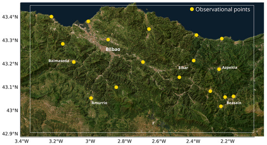
Figure 1.
Study domain and monitoring points. The map shows the location of the city of Bilbao and the surrounding meteorological stations (e.g., Balsameda, Amurrio, Eibar, Azpeitia, Beasain) used in this study.
2.2. Data Sources
This section presents the two main data sources used in this work. First, the numerical simulations produced with the WRF model are described, including their configuration and setup. Then, the observational dataset obtained from a network of meteorological stations is introduced, which serves as ground truth for both the evaluation of the simulations and the training of the machine learning models.
2.2.1. NWP WRF Simulations
As mentioned in Section 1, one part of the proposed framework includes NWP with the aim of improve the raw output from the model. For this purpose, an essential input of the ML model is the data coming from the NWP model output. In this study, WRF (Weather Research and Forecasting) model version 4.6 [14] was used to simulate meteorological variables over the study area. WRF is a non-hydrostatic regional NWP model developed mainly by NCAR (National Center for Atmospheric Research) and its use is not only for research purposes, but also for operational weather forecasting, and its performance and accuracy, particularly for wind resource assessment, has been rigorously evaluated against in-situ measurements [15]. For consistency with the observational dataset, continuous WRF simulations were performed covering a full annual cycle, ensuring that the temporal overlap between simulations and measurements allowed for both the training and validation of the ML models. The simulations provided gridded meteorological wind variables (wind speed and wind direction), which were later used as predictors in the Machine Learning framework. Table 1 summarizes the main configuration of the WRF setup adopted for this study, including domain characteristics, spatial resolution, physical parameterizations, and boundary conditions. The configuration is based on two nested domains, where the inner one corresponds to the d02 (1 km resolution) and the outer one corresponds to the d01 domain. For an easy visualization of the area covered by the WRF model, Figure 2 shows the spatial configuration of the nested domains used in the WRF setup. It should be noted that only the outputs from the d02 domain are used in this study, since this high-resolution domain and fully covers the area where the sensor network is located

Table 1.
Model configuration used for WRF simulations. Domain, period of simulation and physical schemes options selected in this work.
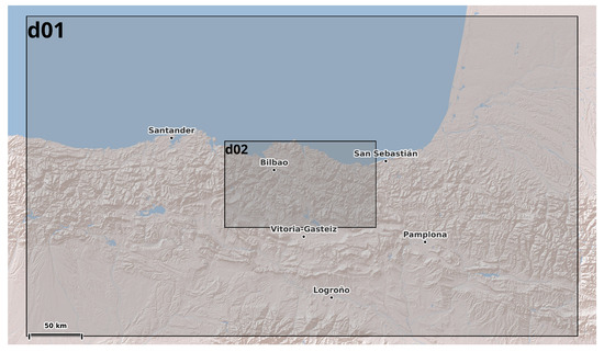
Figure 2.
Configuration of the nested WRF domains used in this study. The outer domain (d01) provides boundary conditions, while the inner domain (d02) corresponds to the high-resolution area.
2.2.2. Observational Data
Observational data are a key element in this study because it provides the real measurements needed to evaluate and improve the performance of models during training. In addition, this approach highlights the importance of having more recent observational data to improve NWP forecasting over the first horizon predictions (the first 24 h). Unlike purely simulated values, observations reflect the actual variability of the atmosphere and ensure that predictions are grounded in reality. Having a well-distributed network of sensors is therefore essential since it allows the model to learn from different local conditions across the study area.
For this work, wind speed and wind direction values were obtained from 18 meteorological stations operated by AEMET (Agencia Estatal de Meteorologia), which is the national meteorology agency of Spain. Table 2 shows the stations metadata within the inner WRF domain (d02). This network covers coastal, urban, and mountainous zones around northern Iberia, areas that are strongly influenced by local orography. Data were collected for a complete year, making it possible to capture seasonal differences and a wide range of meteorological situations. These records were then used to train and validate the machine learning models.
Table 2.
Metadata of the weather observational points. Station code, altitude and geographical coordinates.
2.2.3. Data Processing and Input Vector Structure
This subsection describes how NWP data from WRF and station observations are processed, merged, and transformed to construct a dataset to train the machine-learning models over the entire 1-year period.
First, a spatial and temporal collocation was performed. For each station, WRF variables were extracted at the station location using the nearest grid point for all 18 observational points. All timestamps were converted to UTC and only forecasts matching the observation times were collected. The resulting dataset contained datetime, station metadata (coordinates and altitude), observed variables, and the corresponding WRF wind speed and wind direction predictors as shown in Table 3.
Table 3.
General structure of the training dataset for a forecast horizon h. The table shows how input features are organized into three main categories based to the mathematical notation introduced in this section.
To formally describe the construction of the training dataset, let us define the input feature vector and target variables for a given forecast horizon h (where h). For each station s at time t, the feature vector consists of three main components:
- Station metadata: geographic coordinates and altitude
- WRF model outputs at forecast time t:where ws denotes wind speed, wd wind direction, temp temperature, and p surface pressure.
- Lagged observational features: historical wind measurements from h to 23 h before the forecast time:
Therefore, the complete input vector for a forecast horizon h is constructed as:
The target variables for training are the observed values at time t:
For wind direction, we decompose the angular variable into its zonal (u) and meridional (v) components to handle circularity:
Thus, three independent regression problems are formulated:
- Wind speed model:
- Zonal component model:
- Meridional component model:
After predictions, the corrected wind direction is reconstructed as:
This formulation ensures that for each forecast horizon h, only observational data available at the time of forecast issuance (i.e., measurements up to ) are included in the training and prediction process, emulating realistic operational constraints.
The training dataset and the ML model input variables are based on the scenario in which a forecast is run. For a complete 24 h prediction with NWP model, the latest information from observations is from 1 h before the model is run up to 24 h before; for a 6 h forecast, the most recent observation is 6 h old; and for a 24 h forecast, the last usable data point starts 24 h earlier. The main idea of this work is to construct different datasets that emulate the available information from weather observations to train a total of 24 different models, one for each prediction horizon, taking into account the most recent observational point. To support this explanation, Figure 3 shows a schema of how input vector for each model is constructed, where the available observations decrease according to the lag hours.

Figure 3.
Schematic representation of how observational input vector is constructed for two different target forecast horizon, h = 3 and h = 6.
2.3. Model Training
As described in the previous section, 24 independent datasets were constructed, each corresponding to a forecast horizon between 1 to 24 h according to the last available observational data when a forecast is run. The training procedure was then applied independently to each dataset, ensuring that model development strictly respected the chronological order of the data to emulate realistic operational conditions. For each lead-time dataset, the time series is split chronologically: the first 80% of the samples were used for training, while the 20% were reserved for validation.
The chosen algorithm was the Light Gradient Boosting Machine (LightGBM), which is a gradient-boosted tree ensemble particularly efficient for tabular datasets with heterogeneous predictors. Its ability to capture nonlinear relationships and interactions between variables makes it well-suited for post-processing NWP forecasts.
To refine the models, we performed a randomized search over a predefined hyperparameter space was performed for each dataset and each target variable. The parameters tuned included tree depth, number of leaves, learning rate, number of estimators, and minimum child samples. In addition, the target variables were normalized using min-max normalization fitted only on the training partition. Finally, the training process included an early stopping criterion based on the validation MAE.
As mentioned in the previous section, wind speed (ws) and wind direction (wd) variables were trained separately into the different components.
Two independent LightGBM models were trained, one for the zonal component (u) and another for the meridional component (v). This methodology was applied in order to convert an angular variable such as wind direction into two different scalar variables (x-component and y-component). In addition, the LightGBM does not natively handle the circular nature of directional variables.
In all experiments, a ranking of feature importances, derived from the frequency and gain of variable usage in the ensemble of decision trees was saved. This analysis served to identify which predictors—among lagged observations, WRF forecasts, and station metadata—contributed most to correcting the model errors at different lead times. The overall workflow of the methodology is summarized in Figure 4 as a schema.
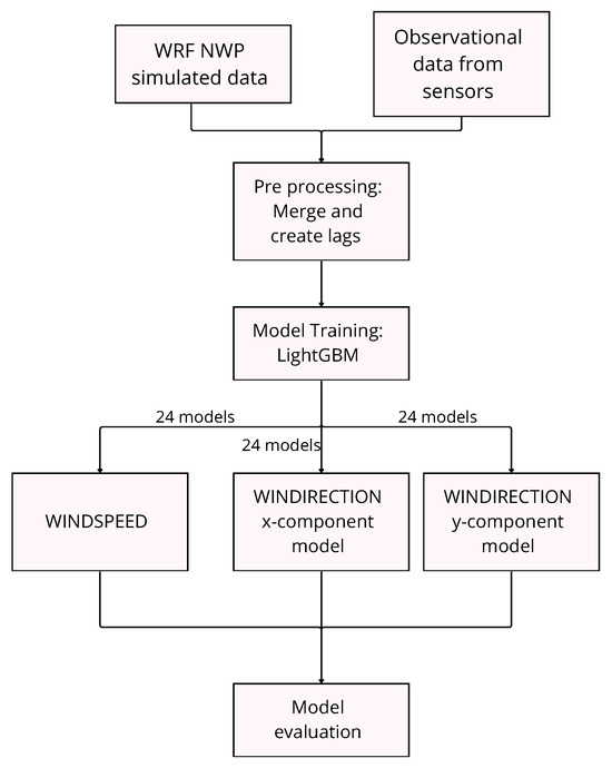
Figure 4.
Data processing and training workflow followed in this work.
2.3.1. Evaluation Test
The evaluation of the proposed framework was carried out through two independent test experiments of 24 h each. These tests were designed to emulate an operational forecasting scenario and to assess the ability of LGBM post-processing to improve the raw WRF output.
Specifically, two consecutive WRF simulations with a 24 h forecast horizon were run, initialized on 20 September 2025 at 00:00 UTC and 21 September 2025 at 00:00 UTC. For each simulation, the trained LGBM models were applied using as input the same type of predictors employed during training, i.e., observational records from the station network combined with the corresponding WRF forecasts. This procedure produced two sets of corrected forecasts for wind speed and wind direction, which were then concatenated to form a continuous time series covering the 48 h evaluation period. The performance of these corrected forecasts was compared against both the raw WRF output and the independent observational data available after the forecast. This comparison allowed us to quantify the improvement achieved by the LGBM post-processing compared to the WRF baseline numerical prediction.
The test performance was evaluated using three complementary metrics: the Mean Absolute Error (MAE), the Root Mean Square Error (RMSE), and the Pearson Correlation Coefficient (R). This combination was selected to offer a robust assessment of both prediction accuracy and skill. The MAE provides a straightforward measure of the average error in the original units (e.g., m/s), while the RMSE is essential for penalizing large errors due to its quadratic formulation. Finally, the Pearson R quantifies the linear correlation between predicted and observed values, confirming the model’s ability to capture the data’s overall trend. Together, these metrics cover error magnitude and relationship strength.
2.3.2. Computational Environment
The development and training of the LightGBM models were performed on a local computational environment. The specifications included an Intel laptop manufactured by HP from China with i5 10th generation processor, 8 cores and 16 GB of RAM. These specifications were deemed sufficient to handle the training of the models for each prediction horizon, leveraging LightGBM’s inherent optimization for multi-core processing. The total process of training all 48 models (24 for wind speed and 24 for the wind direction components u and v combined) required approximately 10 h to complete.
3. Results
This section is divided by three different parts. The first one corresponds to the evaluation of the model performance from a global point of view, showing statistical metrics for wind variables comparing the LGBM prediction results and WRF baseline output. Subsequently, a more in-depth analysis for wind speed and wind direction variables is evaluated separately for the test, showing the improvement with respect to the NWP and the most relevant input features used during model training is presented. Finally, a comparative analysis of the cost functions of the ML model during the training period were carried out to avoid possible overfitting.
3.1. Global Model Performance
To provide an overview of the model performance, Table 4 shows the global performance of the LGBM model compared with the baseline WRF outputs. The aim of this result is to highlight whether the methodology proposed in this work-processing can improve the meteorological forecasts.
Table 4.
Results for the 48 h and 18 observational points test showing MAE, RMSE and R metrics for wind speed and wind direction variables. The best results are highlighted in bold.
Table 4 was constructed by aggregating the results obtained for the 48 h test. For each model and the wind variables, the LGBM predictions and the WRF baseline were evaluated against observations. As shown in the methodology, the mean absolute error (MAE), the root mean square error (RMSE), and the Pearson coefficient (R) were obtained. For wind speed, metrics were calculated directly on the observed values. For wind direction, MAE and RMSE were computed using the minimal angular differences between the predicted and observed directions to properly account for the circular nature of the variable as
where is the wind direction from the local stations and is the corresponding for WRF baseline or LGBM depending what we are comparing. Finally, aggregated values of statistical metrics are calculated by taking into account data from the 18 observational points over the test.
The results demonstrate that the methodology based on LGBM approach improves the forecasts. For wind speed, the ML model decreased the MAE from 2.095 to 0.94 and RMSE from 2.47 to 1.17, while improving R from 0.39 to 0.41. In terms of RMSE, WRF obtained 2.47 and 1.17 for the ML model. The most significant improvement is observed in MAE and RMSE, while the correlation coefficient (R) shows only a marginal increase. This suggests that the ML model effectively reduces the absolute discrepancies with respect to the observations, but it does not capture the temporal trends as accurately as desired. Finally, for wind direction, the ML models halved the MAE, decreasing from to , and reduced the RMSE from to , demonstrating a notable improvement despite the high variability inherent to angular measurements; R was not defined due to the circular nature of the variable. It is important to note the average wind values where the 48 h test took place. In this case, an average of was registered for the wind speed observation across all stations, indicating the tests were conducted in a period characterized by low wind conditions.
Figure 5 presents the MAE improvement for wind speed and wind direction predictions across lead times up to 24 h during the models training period. The results indicate that the ML approach improves wind speed forecasts throughout the entire prediction horizon. The largest improvement is observed at very short-term forecasts, with an improvement exceeding 62% at 1 h ahead, which remains acceptable up to 5 h of prediction, since the model has recent information from observations. After the first few hours, the relative improvement decreases quickly and stabilizes around 53%, remaining nearly constant for the rest of the horizons.
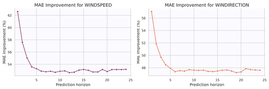
Figure 5.
Evolution of mean absolute error (MAE) improvement respect to the WRF baseline for wind speed and wind direction forecasts across all prediction horizons (1–24 h) and aggregating the 18 observational points.
Finally, predictions for wind direction are provided by the 24 trained models. The improvement is again largest for the shortest lead time, reaching values above 56% at 1 h ahead. However, it decreases rapidly during the first few hours and stabilizes around 48% for longer horizons. This pattern is similar to that observed for wind speed, where the improvement also drops quickly after the initial hours. The rapid decay in relative improvement for both wind speed and wind direction highlights the inherent difficulty of predicting wind values. Figure 5 shows evolution of the Mean Absolute error computed for each 24 forecast horizon for both wind speed and wind direction target variables.
3.2. Wind Speed Analysis
Figure 6 presents a comparative time series of wind speed forecasts from the machine learning (ML) model, the WRF baseline, and actual observations at different 4 of the 18 total stations over the 48 h period. The comparison demonstrates the LGBM model’s superior ability to track the observed wind speed fluctuations closely. Notably, the LGBM forecast effectively captures the timing and amplitude of key wind speed events that the WRF simulation either overestimates. This results visually confirm the quantitative findings presented earlier.
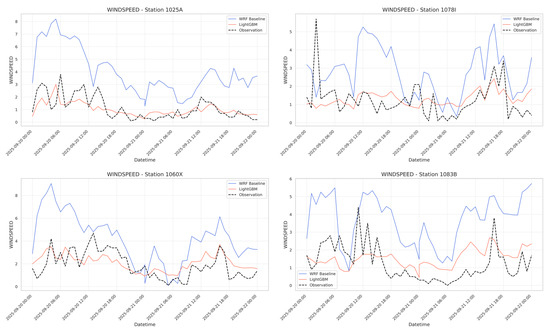
Figure 6.
Time series comparison of wind speed at 4 of the 18 stations during the 48 h evaluation period. The ML-corrected forecasts are compared against the WRF baseline and observations.
Related to the feature importance analysis for wind speed, Figure 7 shows the most important features obtained during the training period corresponding to the models of 1, 8, 16 and 24 h of horizon prediction. Results indicate that for very short lead times, recent lagged wind speed values are among the most influential predictors, together with WRF wind variables. However, as the forecast horizon increases, the relative contribution of lagged values decreases, and other predictors such as wind speed and wind direction from WRF model, relative humidity, and surface pressure gain more importance.
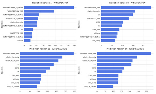
Figure 7.
Feature importance ranking for wind speed models at prediction horizons of 1, 8, 16, and 24 h.
3.3. Wind Direction Analysis
Figure 8 illustrates the wind direction forecasts from the ML model and the WRF baseline against observations at different 4 of the 18 total stations over the 48 h period. The comparison reveals a clear performance differential. The ML model’s forecast demonstrates a remarkably close alignment with the observed wind direction, accurately capturing both the major shifts in wind regime and the finer-scale variability throughout the period. In contrast, the WRF baseline simulation shows significant deviations, frequently failing to replicate the timing and magnitude of directional changes observed in the measurements.
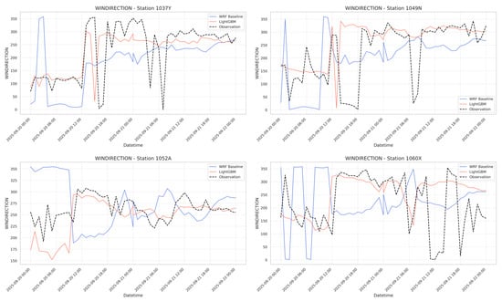
Figure 8.
Time series comparison of wind direction at 4 of the 18 stations during the 48 h evaluation period. The ML-corrected forecasts are compared against the WRF baseline and observations.
Finally, the feature importance analysis was carried out for wind direction. In Figure 9, where the results shows that for very short prediction horizon (1 h), the most recent observations of wind variables, such as wind speed and wind direction are the most influential during the training period, while the prediction horizon increases, the variables coming from the model WRF (wind speed and wind direction as well) and other ones related with the relative humidity and pressure becomes more important.
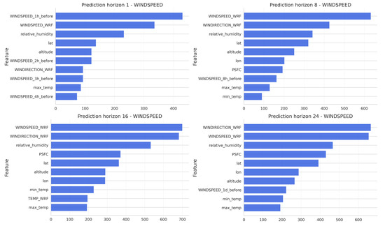
Figure 9.
Feature importance ranking for wind direction models at prediction horizons of 1, 8, 16, and 24 h.
3.4. Training Diagnostics and Convergence
This section presents the loss curves, which illustrate the evolution of the mean absolute error (MAE) during training of the LightGBM regressors, showing both the training set and the independent validation set. These functions of cost are important to assess the convergence of the model and the potential presence of overfitting.
Figure 10 displays the loss curves obtained for wind speed prediction models at different lead times: 1, 8, 16, and 24 h ahead. In all cases, the MAE decreases rapidly during the initial boosting iterations and then progressively flattens, indicating that the model quickly captures the dominant predictive patterns and gradually fine-tunes residual errors. As expected, the absolute value of MAE is slightly higher for longer forecast horizons (e.g., 16–24 h) compared to shorter ones (1 h), reflecting the increasing intrinsic difficulty of prediction for longer horizons. The relative alignment of the training and validation curves indicates that the models maintain generalization capacity and do not suffer from overfitting, even when the number of boosting iterations increases. However, it is observed that the validation loss curve remains lower than the training one. While atypical, this behavior suggests that the validation dataset for wind speed contains samples that are inherently easier to predict or present less variance than the training set, leading to a higher model-observation agreement. It should be noted that this favorable condition might be specific to the wind speed variable and does not necessarily imply similar behavior for wind direction.
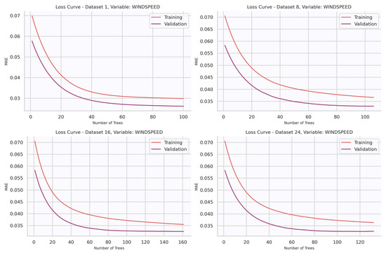
Figure 10.
Loss curves for wind speed models trained at forecast horizons of 1, 8, 16, and 24 h.
Similarly, Figure 11 presents the angular loss curves for wind direction prediction at different lead times: 1, 8, 16, and 24 h ahead. In this case, the metric reported is the angular mean absolute error (MAE), which quantifies directional discrepancies in degrees. As with wind speed, the curves show a steep initial decrease followed by progressive stabilization, indicating effective learning of the main predictive signals during the first boosting iterations. Moreover, a clear dependence on the forecast horizon is observed, with errors increasing from shorter (1 h) to longer (16–24 h) lead times. The parallel behavior of training and validation curves also suggests that the models achieve good convergence without signs of overfitting.
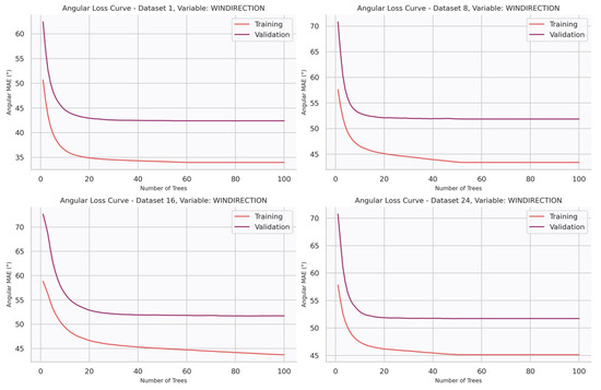
Figure 11.
Loss curves for wind direction models trained at forecast horizons of 1, 8, 16, and 24 h.
4. Discussion
In this study, we have developed and evaluated a post-processing Machine Learning correction framework based on the LightGBM regressor to improve short-term wind predictions made by the WRF model. We used observational data (wind speed and direction), together with WRF outputs and other meteorological predictors like surface pressure, relative humidity, and geographical coordinates to train different models for forecast horizons from 1 to 24 h training the models with the most recent measurement. The results demonstrate our hypothesis formulated in Section 1, which states that machine learning post-processing can substantially enhance short-term wind forecasts derived from numerical weather prediction models. During the evaluation test, the LightGBM-based correction notably reduced both mean absolute error (MAE) from 2.095 m/s to 0.94 m/s in the case of wind speed and from to in the case of wind direction over the WRF baseline. The root mean square error (RMSE) metric also improves for wind speed and direction variables. The LGBM model reduces the wind speed RMSE from 2.47 m/s to 1.17 m/s representing a 52.6% improvement over the WRF baseline, and outperforming the 26.1% improvement reported by [13] using XGBoost-based bias correction (from 1.80 m/s to 1.33 m/s). In addition, as this approach uses the most recent local measurements available from sensors, the improvement was particularly marked for the first forecast hours, which aligns with the higher availability of recent data. Average wind speed values during the 48 h test period revealed an average wind speed observation of , and accordingly, low wind speeds are critical in the impact on the grid capacity, as thermal models by [6,7] suggest that small increases in wind speed within this low range lead to a significant increase in the conductor capacity.
Despite the overall improvement, the correlation coefficient (R) showed only marginal increases, rising from 0.39 to 0.41 with respect to the WRF reference for wind speed forecasts. This implies that while the LightGBM correction effectively reduces amplitude errors, it does not fully reproduce the temporal phase of observed fluctuations. This is probably due to the evaluation metric used during the models training, which was the MAE metric. This means that the optimization process focused on minimizing the average magnitude of the errors rather than maximizing the temporal agreement between the predicted and observed series.
Time series results obtained for the test period demonstrate that the LightGBM model acts as a statistical post-processing tool that reduces the systematic errors present in the baseline WRF forecasts. Rather than replacing WRF or operating as an independent forecasting system, the ML component enhances the short-term accuracy of the numerical model by correcting its local biases. by correcting systematic biases and integrating local observations not fully resolved by the numerical model. Furthermore, the examination of the loss curves during the training and validation phase demonstrates a similar convergence across both datasets. This convergence pattern indicates that the approach does not overfit, demonstrating that LightGBM architecture has successfully learned the intrinsic, non-linear atmospheric dynamics from the input features.
5. Conclusions and Future Work
This work presented a hybrid framework that combines numerical weather prediction and machine learning to enhance short-term wind forecasts for energy management applications. The proposed methodology integrates mesoscale model outputs with real-time observations from a distributed sensor network, forming a simplified representation of a real-time sensor-based system. In addition, it should be noted that the machine learning component does not operate independently from the numerical model; it functions as a post-processing correction step that refines the original WRF forecasts rather than replacing them. The machine learning correction, implemented using a LightGBM regressor, achieved substantial improvements, reducing the mean absolute error for wind speed and wind direction by more than 60% and 50%, respectively. These results confirm that local, high-frequency observational data play a decisive role in mitigating systematic biases in numerical forecasts, particularly during the first forecast hours, which are the most critical for operational decision-making. By coupling environmental sensing and data-driven modelling, this framework also illustrates the potential of IoT- and WSN-based approaches to enhance energy efficiency through improved meteorological awareness.
Although the results obtained are highly positive, this study also presents certain limitations, mainly related to the short duration of the evaluation test period. Therefore, future work will extend the testing phase to a longer time span and under diverse meteorological conditions. In addition, the proposed approach opens several promising research directions, such as evaluating the generalizability of the trained models across different domains or determining whether a model trained in one region can be effectively transferred to another. Further work will also explore alternative regressors and machine learning techniques to compare their performance within the same hybrid framework.
Author Contributions
Conceptualization, A.P.P.; Data curation, A.P.P.; Formal analysis, A.P.P.; Methodology, A.P.P.; Visualization, A.P.P.; Project administration, J.A.C.V. and A.J.J.V.; Supervision, J.A.C.V. and A.J.J.V.; Writing—original draft, J.A.C.V.; Writing—review and editing, A.J.J.V.; Funding acquisition, A.J.J.V. All authors have read and agreed to the published version of the manuscript.
Funding
This research received no external funding.
Data Availability Statement
The original contributions presented in the study are included in the article, further inquiries can be directed to the corresponding author.
Conflicts of Interest
The authors declare no conflicts of interest.
Abbreviations
The following abbreviations are used in this manuscript:
| DLR | Dynamic Line Rating |
| GET | Grid-Enhancing Technology |
| TSOs | Transmission System Operators |
| DSOs | Distribution System Operators |
| OHL | Overhead Line |
| SLR | Static Line Rating |
| NWP | Numerical Weather Prediction |
| WRF | Weather Research and Forecasting |
| LightGBM | Light Gradient Boosting Machine |
| ML | Machine Learning |
| MAE | Mean Absolute Error |
| RMSE | Root Mean Square Error |
| R | Pearson Correlation Coefficient |
| IEEE | Institute of Electrical and Electronics Engineers |
| CIGRE | Conseil International des Grands Réseaux Électriques |
References
- Günay, M. Forecasting annual gross electricity demand by artificial neural networks using predicted values of socio-economic indicators and climatic conditions: Case of Turkey. Energy Policy 2016, 90, 92–101. [Google Scholar] [CrossRef]
- Brożyna, J.; Lu, J.; Strielkowski, W. Is European current climate regulation strategy feasible? A comparative analysis of “Fit for 55” green transition package for V4 and LEU4. Energy Strategy Rev. 2025, 61, 101843. [Google Scholar] [CrossRef]
- Gyimah, J.; Han, Y.; Yao, X. Renewable energy consumption, good governance system, economic growth, and FDI: The pathway towards environmental quality in European countries. Energy 2025, 337, 138708. [Google Scholar] [CrossRef]
- Wu, K.; Wang, L.; Ha, H.; Wang, Z. Dynamic line rating and optimal transmission switching for maximizing renewable energy sources injection with voltage stability constraint. Appl. Energy 2025, 378, 124651. [Google Scholar] [CrossRef]
- Fernandez, E.; Albizu, I.; Bedialauneta, M.; Mazon, A.; Leite, P. Review of dynamic line rating systems for wind power integration. Renew. Sustain. Energy Rev. 2016, 53, 80–92. [Google Scholar] [CrossRef]
- IEEE 738-2012; IEEE Standard for Calculating the Current-Temperature Relationship of Bare Overhead Conductors. IEEE/Institute of Electrical and Electronics Engineers Incorporated: Piscataway, NJ, USA, 2012.
- Iglesias, J.; Watt, G.; Douglass, D.; Morgan, V.; Stephen, R.; Bertinat, M.; Muftic, D.; Puffer, R.; Guery, D.; Ueda, S.; et al. Guide for Thermal Rating Calculations of Overhead Lines; CIGRE Technical brochure N° 601; CIGRE: Paris, France, 2014; Available online: https://hdl.handle.net/2268/178855 (accessed on 20 April 2025).
- EL-Azab, M.; Omran, W.; Mekhamer, S.; Talaat, H. Congestion management of power systems by optimizing grid topology and using dynamic thermal rating. Electr. Power Syst. Res. 2021, 199, 107433. [Google Scholar] [CrossRef]
- Michiorri, A.; Nguyen, H.M.; Alessandrini, S.; Bremnes, J.B.; Dierer, S.; Ferrero, E.; Nygaard, B.E.; Pinson, P.; Thomaidis, N.; Uski, S. Forecasting for dynamic line rating. Renew. Sustain. Energy Rev. 2015, 52, 1713–1730. [Google Scholar] [CrossRef]
- Zhang, Z.; Teh, J. Enhancing grid flexibility and renewable integration: A review of V2G and dynamic line rating synergies. Renew. Sustain. Energy Rev. 2026, 226, 116341. [Google Scholar] [CrossRef]
- Pujante Pérez, A.; Martínez-Abarca, C.; Valdés, J.A.C.; Fernández, E.I.; Valera, A.J.J. Optimization of Energy Infrastructure Through High-Resolution Weather Forecasting. In Proceedings of the International Conference on Ubiquitous Computing and Ambient Intelligence (UCAmI 2024), Belfast, UK, 27–29 November 2024; Bravo, J., Nugent, C., Cleland, I., Eds.; Springer: Cham, Switzerland, 2024; pp. 773–778. [Google Scholar]
- Zhou, S.; Gao, C.Y.; Duan, Z.; Xi, X.; Li, Y. A robust error correction method for numerical weather prediction wind speed based on Bayesian optimization, variational mode decomposition, principal component analysis, and random forest: VMD-PCA-RF (version 1.0.0). Geosci. Model Dev. 2023, 16, 6247–6266. [Google Scholar] [CrossRef]
- Fang, Y.; Wu, Y.; Wu, F.; Yan, Y.; Liu, Q.; Liu, N.; Xia, J. Short-term wind speed forecasting bias correction in the Hangzhou area of China based on a machine learning model. Atmos. Ocean. Sci. Lett. 2023, 16, 100339. [Google Scholar] [CrossRef]
- Skamarock, W.C.; Klemp, J.B.; Dudhia, J.; Gill, D.O.; Liu, Z.; Berner, J.; Wang, W.; Powers, J.G.; Duda, M.G.; Barker, D.M.; et al. A Description of the Advanced Research WRF Model Version 4; The National Center for Atmospheric Research: Boulder, CO, USA, 2019; Volume 145, p. 550. [Google Scholar]
- Fernández-González, S.; Martín, M.L.; García-Ortega, E.; Merino, A.; Lorenzana, J.; Sánchez, J.L.; Valero, F.; Rodrigo, J.S. Sensitivity analysis of the WRF model: Wind-resource assessment for complex terrain. J. Appl. Meteorol. Climatol. 2018, 57, 733–753. [Google Scholar] [CrossRef]
Disclaimer/Publisher’s Note: The statements, opinions and data contained in all publications are solely those of the individual author(s) and contributor(s) and not of MDPI and/or the editor(s). MDPI and/or the editor(s) disclaim responsibility for any injury to people or property resulting from any ideas, methods, instructions or products referred to in the content. |
© 2025 by the authors. Licensee MDPI, Basel, Switzerland. This article is an open access article distributed under the terms and conditions of the Creative Commons Attribution (CC BY) license (https://creativecommons.org/licenses/by/4.0/).