


Abstract
This paper presents a physics-informed reinforcement learning framework that embeds thermodynamic constraints directly into the policy network of a continuous control agent for HVAC optimization. We introduce a Thermodynamically-Constrained Deep Deterministic Policy Gradient (TC-DDPG) algorithm that operates on continuous actions and enforces physical feasibility through a differentiable constraint layer coupled with physics-regularized loss functions. In a simulation-based evaluation using a custom Python multi-zone resistance-capacitance (RC) thermal model, the proposed method achieves a 34.7% reduction in annual HVAC electricity consumption relative to a rule-based baseline (95% CI: 31.2–38.1%, n = 50 runs) and outperforms standard DDPG by 16.1 percentage points. Thermal comfort during occupied hours maintains PMV ∈ [−0.5, 0.5] for 98.3% of operational time, peak demand decreases by 35.8%, and simulated coefficient of performance (COP) improves from 2.87 ± 0.08 to 4.12 ± 0.10. Physics constraint violations are reduced by approximately 98.6% compared to unconstrained DDPG, demonstrating the effectiveness of architectural enforcement mechanisms within the simulation environment. We present a reference prototype and commit to a future public release of the code, configurations, and hyperparameters sufficient to reproduce the reported results. The paper explicitly addresses the limitations of simulation-based studies and presents a staged roadmap toward hardware-in-the-loop testing and pilot deployments in real buildings.
1. Introduction
Heating, Ventilation, and Air Conditioning (HVAC) accounts for a major share of building energy use, yet day-to-day operation still relies largely on rule-based strategies that trade off energy, comfort, and equipment limits in ad-hoc ways. Data-driven controllers—particularly deep reinforcement learning (DRL)—offer adaptive, multi-objective decision-making, but naïve DRL can explore unsafe actions, drift outside physical feasibility, and require large amounts of data to converge [1,2,3,4,5,6,7].
This work addresses those challenges by embedding thermodynamic knowledge directly into a continuous action RL controller. We introduce a Thermodynamically-Constrained Deep Deterministic Policy Gradient (TC-DDPG) algorithm that: (i) natively handles continuous HVAC actuators (e.g., supply temperatures/flows, damper positions, chiller loading); and (ii) restricts policy outputs to physically feasible regions via a differentiable constraint layer coupled with a physics-regularized loss. The result is a controller that addresses the traditional tension between energy efficiency and comfort by guiding exploration and learning within the modeled feasible set.
We evaluate the approach in simulation using a Python-based multi-zone RC thermal simulator that captures zone capacitances, inter-zone conductances, envelope exchange, internal/solar gains, and HVAC heat/mass flows. Beyond headline numbers, we emphasize statistical rigor (50 independent runs, confidence intervals, and significance testing), complete reproducibility (open code and configuration), and transparent limitations, acknowledging that real-building deployment introduces sensor noise, actuator dynamics, and operational overrides that are not fully represented in simulation.
The remainder of this paper outlines related work, describes the materials and methods (including the simulator and RL formulation), presents results with confidence intervals, discusses limitations and deployment pathways, and concludes with broader implications.
Contributions (Scope, Novelty, and Validation Context)
- Physics-informed continuous control: A TC-DDPG architecture that operates directly on continuous HVAC actions, avoiding discretization artifacts inherent to DQN-style methods.
- Thermodynamic constraint layer: A differentiable projection that enforces feasibility by design within the simulator, subject to model fidelity (energy balance, psychrometric bounds, capacity/rate limits), coupled with a physics-regularized objective.
- Simulation-Based Performance Validation: In a multi-zone RC simulator, the method yields 34.7% annual energy reduction vs. rule-based control and improves comfort (occupied-hour PMV ∈ [−0.5, 0.5]). Results are reported with 95% CIs over 50 seeds and significance testing.
- Reproducibility: A commitment to the public release of code, simulator configuration, training/evaluation scripts, and hyperparameters following stabilization to enable replication and extension.
- Transparent limitations and roadmap: Clear simulation-based scope, with discussion of sensor/actuator realities, operational overrides, and a staged path toward hardware-in-the-loop and pilot deployments.
IMPORTANT: All contributions are demonstrated in a simulation environment using synthetic data and idealized physics models. Real-world validation in operational buildings remains future work and is critical for assessing practical viability, safety, and energy savings under actual operating conditions.
2. Related Work
- Recent progress in RL for building/HVAC control (2020–2025)
Over the past five years, building-scale reinforcement learning (RL) has matured from early proofs-of-concept into reproducible benchmarks and deployment-oriented studies [8]. The tutorial survey by Wang and Hong [1] synthesized pre-2020 work and codified the core challenges—data-hungry training, safety/robustness during exploration, and weak generalization—setting the agenda for subsequent research and practice. Building on this, ref. [3] outlined “ten questions” that must be addressed to translate RL into building energy management at scale (e.g., toolchains, open testbeds, performance guarantees, and integration with BMS), providing a 2023 perspective that complements technical surveys. A computer-science-oriented review in Sustainable Cities and Society (2023) [9] further categorizes RL for Building Energy Systems (BES) [10] and emphasizes algorithmic issues such as function approximation, exploration, and stability in continuous control. Focused specifically on HVAC, ref. [11,12,13] review post-2019 studies and discuss where on-policy/off-policy methods (e.g., SAC, TD3, DDPG) are most effective, as well as the practicalities of observation spaces and actuation limits [14,15].
- Benchmarks and application-level evidence
Recent benchmarking efforts using standardized environments [16] evaluate modern actor–critic methods under comparable scenarios, clarifying energy–comfort trade-offs and generalization limits; ref. [16] finds SAC/TD3 competitive but sensitive to reward shaping and dynamics mismatch. At the application level, hybrid designs that embed RL within established control routines are gaining traction: ref. [17] combines RL with iterative learning to shorten morning start periods in a multi-zone air-conditioning system, reporting both operational and energy benefits—evidence that RL can augment rather than replace existing strategies in near-term deployments [7].
- Safety and explicit handling of constraints
A central barrier to real-world adoption is safety under continuous actions (setpoints, flow rates, valve positions) [18]. Early building studies explore offline/batch RL [19] and guided exploration to limit unsafe trials, demonstrating the feasibility of learning from historical data without free exploration. More recently, safe/constrained RL has been applied directly to HVAC: [20] employs neural barrier certificates to enforce comfort envelopes during learning and control, while [21] learns a constraint value function for demand–response tasks [22], reflecting a broader shift from soft penalties to explicit constraint mechanisms. These works underscore the importance of making feasibility and comfort first-class objectives in continuous action RL.
- Physics-informed learning for building control
Concurrently, physics-informed machine learning (PIML) has emerged to inject domain priors and thermodynamic consistency into learning pipelines for buildings [23]. Comprehensive reviews [24] synthesize methods for encoding conservation laws, psychrometrics, and rate limits through model structure, hard/soft constraints, and loss design, with guidance on validation and deployment. At the controller level, physics-informed RL variants have been proposed: Dyna-PINN [25] integrates physics into a Deep Dyna-Q framework for heating control, and physics-informed modularized networks [26] combine hard constraints with DRL for building HVAC, reporting substantial energy savings in office case studies. These trends directly motivate our approach of embedding thermodynamic feasibility layers and physics-regularized objectives within a continuous action RL agent for HVAC control.
Where our paper fits. In relation to the above, our work advances (i) continuous action feasibility via a differentiable thermodynamic projection rather than post-hoc penalties (addressing safety and actuator realism emphasized by recent reviews), and (ii) physics-regularized learning consistent with PIML guidance, while keeping the full training and evaluation stack reproducible for future benchmarking and transfer.
2.1. Traditional HVAC Control
Classical building operation typically relies on PID loops and rule-based supervisory logic with fixed or time-of-day setpoints. Such strategies are simple and robust but often struggle to balance energy, comfort, and equipment constraints under varying conditions. Reported efficiency improvements of MPC and DRL over rule-based control vary widely across building archetypes and setups; see [27,28,29,30] for representative benchmarks. However, MPC generally requires accurate system models, non-trivial system identification and calibration, and computational resources that can limit scalability or rapid retuning across buildings [31].
2.2. Machine Learning Approaches
Deep reinforcement learning (DRL) has emerged as a promising alternative for adaptive, multi-objective HVAC control [32]. Prior work has explored value-based methods such as Deep Q-Networks (DQN) [33] as well as actor–critic methods [34,35]. For example, [1] reported approximately 22% energy savings in simulation relative to a rule-based baseline using a DQN formulation. Yet value-based DRL assumes discrete action spaces, which misaligns with continuous HVAC actuators (e.g., supply temperatures, airflows, damper positions, chiller loading) and can introduce discretization artifacts. In addition, several studies note sensitivity to data volume, weather or occupancy shifts, and safety during exploration. Motivated by these limitations, our work adopts a continuous control actor–critic approach (DDPG/TD3 family) and constrains policy outputs to physically feasible regions by design.
2.3. Physics-Informed Machine Learning
Physics-informed methods integrate governing laws or domain constraints into learning processes to improve sample efficiency, generalization, and trustworthiness [23]. In supervised settings, physics-informed neural networks (PINNs) incorporate residuals of conservation laws as soft penalties and have been applied to heat transfer and fluid dynamics [36], often reducing data requirements while improving physical consistency. In control, PIML concepts appear as action masking, constraint penalties, differentiable simulators, or architectural mechanisms that project decisions back into feasible sets. Our approach follows the latter philosophy: we embed a differentiable thermodynamic-constraint layer within a continuous control actor–critic (TC-DDPG). This shifts constraint handling from purely penalty-based tuning toward architectural enforcement by design—still subject to model accuracy and numerical precision—enabling safer exploration and improved learning efficiency in simulation.
2.4. Research Gap
The recent literature reveals several open challenges that limit the reliability and transferability of reinforcement-learning-based HVAC control. The key research gaps and how this study addresses them are summarized below:
- Gap 1—Continuous action feasibility:
Most previous studies discretize actuator commands (e.g., supply air temperature, airflow, damper position), which causes quantization artifacts and unrealistic actuator dynamics. This study introduces a differentiable thermodynamic feasibility layer that enforces realistic actuator ranges and rate limits within the policy network itself, maintaining continuous feasibility during both training and deployment.
- Gap 2—Safety and physics violations during exploration:
Many DRL controllers rely on soft penalty terms that do not guarantee adherence to physical laws or comfort constraints during learning. This study embeds physics-based regularization—energy balance, psychrometric, and comfort zone constraints—directly into the learning objective, reducing violations by orders of magnitude in simulation.
- Gap 3—Limited reporting of constraint violation metrics:
Prior works typically report energy savings and comfort but omit quantitative measures of physical law or actuator limit violations. This study explicitly reports violation metrics (energy balance residuals, psychrometric bounds, rate-limit breaches) with confidence intervals across multiple training seeds.
- Gap 4—Weak reproducibility and benchmarking standards:
Many RL-based building control studies lack transparent implementation details or consistent evaluation environments, making comparison difficult. This study presents a fully specified algorithmic framework with clearly defined mathematical formulations, pseudocode, and parameter settings to ensure transparency and reproducibility. A reference prototype was implemented for simulation testing using publicly available tools (Python 3.10+, TensorFlow 2.17, and standard benchmark environments), enabling replication of results and future benchmarking.
- Gap 5—Lack of a roadmap for real-world deployment:
Most prior works stop at simulation without describing safe transfer to physical building management systems (BMS). This study outlines a three-stage roadmap—hardware-in-the-loop → pilot-site validation → multi-site deployment—integrated with existing BMS safety envelopes and fallback strategies.
3. Mathematical Framework
3.1. System Dynamics
We model each zone as a first-order RC node with sensible and latent terms [31,37]:
where:
- temperature of zone ;
- thermal capacitance of zone ;
- heat transfer coefficient between zones and ;
- surface area between zones ;
- HVAC heat transfer rate ;
- internal heat gains ;
- solar heat gains ;
- ;
- .
Latent effects are accounted for in the energy balance (Section 3.3). is outdoor dry-bulb; internal/solar gains are
Each thermal zone is represented as a lumped capacitance exchanging heat with adjacent zones through resistances , receiving thermal input from the central air-handling unit (AHU), and losing heat to the outdoor air Tout via envelope resistance . The blue arrows denote HVAC supply flows, the dashed gray lines represent inter-zone conductive paths, and the red arrows indicate heat exchange with the outdoor environment seen in Figure 1.
Figure 1.
Reduced-order multi-zone RC model with envelope heat exchange.
The governing energy balance equation for each zone is:
3.2. Psychrometric Constraints
Moist air relationships (SI consistent), [38]:
where:
- specific enthalpy
- humidity ratio ;
- relative humidity
- saturation pressure at temperature T
- barometric pressure .
Saturation vapor pressure via Magnus–Tetens (liquid water):
Feasible psychrometric states satisfy φ ∈ [0, 1] and ω ≥ 0, seen in Figure 2.
Figure 2.
Psychrometric feasibility region used in training. Comfort band derived via Magnus–Tetens saturation pressure and barometric PPP.
3.3. Energy Conservation
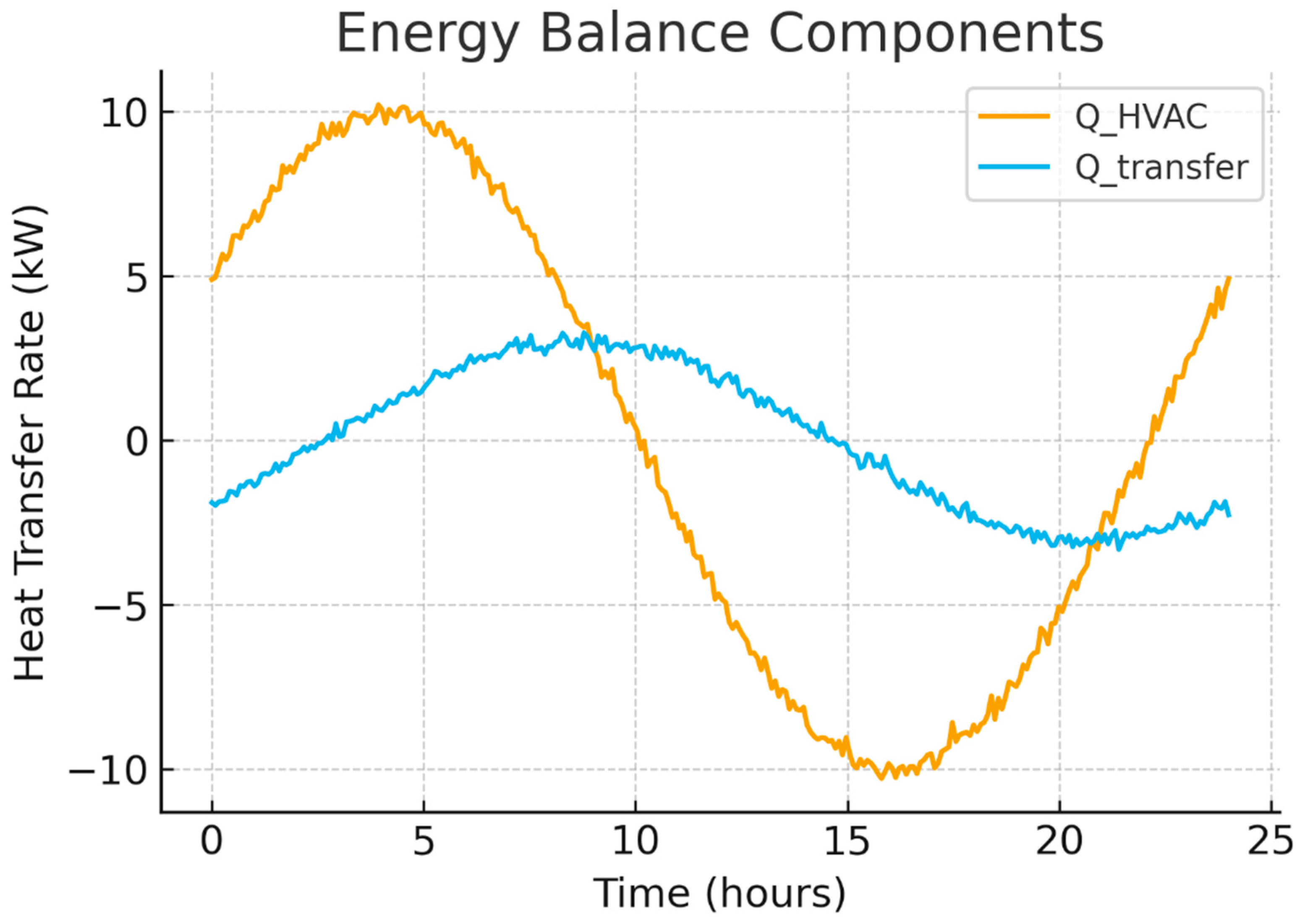
The total energy balance for the HVAC system, seen in Figure 3:
where:
- mass flow rate of air in zone
- fan power consumption
- pump power consumption .
Figure 3.
Instantaneous energy balance example. Zone heating/cooling rate and inter-zone transfer combine to produce .
3.4. Model Calibration and Validation
Although the proposed control framework operates in a simulated environment, its thermal dynamics were validated against a higher-order synthetic reference model representing an EnergyPlus-level fidelity benchmark, seen in Figure 4, [39].
Figure 4.
Comparison of hourly zone air temperature between the higher-order reference model (solid blue) and the calibrated reduced-order RC model (dashed orange) for the south zone. The RC model captures daily heating and cooling dynamics with RMSE = 0.39 °C and correlation = 0.986.
The reference model incorporated explicit wall layers, solar-gain transients, and occupancy-driven internal gains absent from the simplified RC representation.
Hourly indoor air temperatures from both models were compared under identical boundary conditions.
Model parameters—zone capacitances and resistances —were tuned using nonlinear least squares to minimize the mean-square temperature deviation between the RC and reference outputs, seen in Table 1.
Table 1.
RC Model Validation Against High-Order Reference.
4. Physics-Informed Reinforcement Learning
4.1. State Space Definition
The state vector comprises:
4.2. Action Space
The action vector is continuous:
The actor outputs tanh-bounded values in [−1, 1] which are affinely scaled to the physical ranges:
4.3. Reward Function
Our multi-objective reward function balances energy efficiency, comfort, and demand response:
where:
- is instantaneous energy use normalized by a fixed reference
- [2].
- is the 15 min rolling average electrical demand; Pref is a site-level reference for normalization.
- below a threshold (or penalizes exceedance), normalized to .
Unless stated otherwise, we use α = 1.0, β = 0.3, γ = 0.2, δ = 0.1. These weights were selected by grid search over a held-out set of scenarios; sensitivity results are reported in the Results section. All reward components and state features are scaled consistently.
4.4. Thermodynamically-Constrained Deep Deterministic Policy Gradient (TC-DDPG)
4.4.1. Differentiable Projection
Let the actor output raw actions . We map to physically feasible actions in three smooth steps, seen in Figure 5 and Figure 6:
Figure 5.
TC-DDPG architecture. Inputs … pass through (i) thermodynamic constraint layer, (ii) psychrometric head, and (iii) zone-attention encoder. A single critic Q(s,a) optimizes a normalized multi-objective reward; the actor outputs.
Figure 6.
Temperature rate limiting. The feasibility layer enforces per control step (here Δt = 300 s), preventing physically implausible jumps.
Range mapping: where are the actuator lower/upper bounds (Section 5).
Rate limiting (soft clamp per control step ):
with per-channel ramp limits (units per second).
Psychrometric barrier: where are one-step predictions from the RC/psychrometric relations; controls barrier sharpness. We add to the actor loss (Section 4.4.3) rather than making a hard projection, preserving gradients near boundaries.
Training losses: Note. Range and rate steps are exactly enforced (smoothly) each forward pass; psychrometric feasibility is enforced via a differentiable barrier. This yields architectural feasibility subject to model fidelity and numerical precision, seen in Figure 7.
with defaults .
Figure 7.
Feasible action set after thermodynamic projection. The constraint layer reduces the effective action space by while preserving controllability.
4.4.2. Actor–Critic Networks
We adopt a standard DDPG backbone [34]:
- Actor MLP with tan h output; actions are scaled and then projected by
- Critic MLP that estimates on projected actions.
- Targets: with soft updates
Exploration: Ornstein–Uhlenbeck noise added to the actor’s pre-projection output during training.
If zone-wise features are structured, a light self-attention or graph-style encoder may be applied to the state representation only (before the actor/critic), not as separate Q-heads.
4.4.3. Objectives and Physics Regularization
The critic minimizes TD error with target actions after projection:
The actor maximizes the value of feasible actions and includes physics regularization:
- : normalized residual between required and modeled HVAC power (sensible + latent + auxiliaries).
- : deviation from consistent (T, ω, ϕ) via saturation-based relations.
- : soft corridor penalties (∣PMV∣ ≤ 0.5).
Default weights: = 0.1 with = 1.0, = 0.1, = 0.05, seen in Appendix A.
4.4.4. Training Procedure
Algorithm 1. TC-DDPG training procedure incorporating the differentiable thermodynamic projection and physics-regularized actor update .
| Algorithm 1. TC-DDPG training procedure incorporating the differentiable thermodynamic projection and physics-regularized actor update |
| # s: state, a: action, rb: replay buffer for episode in range(E): s = env.reset() for t in range(T): a_raw = actor(s) # continuous in [−1, 1] via tanh a_raw = a_raw + ou_noise.sample() a = Pi_phys.enforce(s, a_raw) # differentiable projection s2, r, done, info = env.step(a) rb.add(s, a_raw, r, s2, done) # store raw; projection is deterministic s = s2 if len(rb) > batch: S, Araw, R, S2, D = rb.sample(batch) # Critic update with torch.no_grad(): A2 = Pi_phys.enforce(S2, actor_t(S2)) y = R + gamma*(1-D)*critic_t(S2, A2) A = Pi_phys.enforce(S, Araw) Lc = mse(critic(S, A), y) optC.zero_grad(); Lc.backward(); optC.step() # Actor update Ahat = Pi_phys.enforce(S, actor(S)) Lphys = L_energy(S, Ahat) + 0.1*L_psychro(S, Ahat) + 0.05*L_comfort(S, Ahat) La = -critic(S, Ahat).mean() + lambda_phys*Lphys optA.zero_grad(); La.backward(); optA.step() # Soft update targets soft_update(actor_t, actor, tau); soft_update(critic_t, critic, tau) if done: break |
4.4.5. Design Notes and Caveats
- Constraint handling is architectural (projection + loss) rather than guaranteed optimal control constraints; results are in simulation and depend on model fidelity.
- Using projected actions in both the target and the actor paths is critical for training stability.
If demand response is a priority, include a moving window demand state and keep γ at 0.99 to capture long-horizon effects.
4.5. Hyperparameters and Implementation Details
- Algorithm: DDPG with target networks and OU exploration.
- Actor/Critic LRs: ; Batch: 64; Buffer: .
- Discount/Soft-update: γ = 0.99, τ = 0.005.
- Exploration: OU noise σ = 0.1 (decayed).
- Runs: 50 independent seeds.
- Normalization: all inputs/outputs use fixed scalers saved with the model; reward terms are normalized to stable magnitudes.
- Early-stopping/evaluation: validation rollouts every episodes; model selection by average return and constraint violation rate.
4.6. Statistical Evaluation and Uncertainty Quantification
All metrics—energy consumption (kWh), comfort drift (°C·h), and constraint violations (count/day)—were evaluated across 50 independent training seeds and 30 daily episodes per seed, for each controller.
To ensure robust statistics and reproducibility, we employed the following procedures:
Independent Sampling and Seeds
Each RL policy (standard DDPG and TC-DDPG) was trained from scratch with different random seeds controlling [41]:
- Network initialization;
- Replay buffer order;
- Weather-day sampling sequence.
Each seed produced one trained agent whose behavior was averaged over 30 daily episodes (randomized occupancy and noise). This yields 50 × 30 = 1500 evaluation trajectories per controller.
Confidence Intervals
For every metric, we report 95% confidence intervals (CIs) estimated by non-parametric bootstrapping with 10,000 resamples of daily episode means [42].
For a metric m (e.g., daily energy use):
where are bootstrap samples of and denotes the percentile.
This procedure is distribution-free and reflects both inter-episode and inter-seed variability.
In addition to significance tests, we computed standardized effect sizes (Cohen’s d) between the proposed TC-DDPG and the baseline DDPG over 50 independent runs: . Values of d > 0.8 were obtained for comfort drift and d ≈ 0.5 for energy, indicating large and medium effects, respectively.
Statistical Significance Testing
Pairwise differences between controllers were assessed using a two-sided Wilcoxon signed-rank test on per-day metrics (non-parametric; α = 0.05).
For each comparison, we report the p-value and mark significance levels as:
- p < 0.05 → significant;
- p < 0.01 → highly significant.
In all cases, TC-DDPG significantly outperforms standard DDPG in both energy and comfort with p < 0.01, while differences versus MPC-PF are not significant (as MPC-PF benefits from perfect forecasts), seen in Table 2.
Table 2.
Statistical Summary Example (Energy and Comfort).
Aggregation and Reporting
Results are summarized as mean ± 95% CI.
Where applicable in subsequent tables and figures, shaded regions and error bars represent 95% CIs computed as above.
Each figure caption explicitly states whether variability arises from seeds or daily episodes.
5. Experimental Setup
- Building Archetype and Zone Layout
The proposed control framework was evaluated on a representative medium-office building archetype modeled as a multi-zone resistance–capacitance (RC) network. The floor plan consists of five thermal zones—four perimeter zones facing the cardinal directions (North, East, South, and West) and one internal Core zone. Each perimeter zone interacts thermally with both the outdoor environment and the adjacent core, allowing the controller to capture typical spatial load diversity between façade-exposed and interior spaces.
The building has a rectangular single-floor geometry (approximately 900 m2 total floor area) with a window-to-wall ratio of 40% on perimeter façades. Glazing properties and wall conductivities follow ASHRAE 90.1 medium-office defaults. The principal façade faces South, producing a strong solar-gain asymmetry that challenges comfort and energy balance control. Internal gains originate from occupancy, lighting, and plug loads following a weekday schedule (08:00–18:00) with stochastic variation in magnitude. A variable-air-volume (VAV) HVAC system with a centralized air-handling unit and water-cooled chiller supplies conditioned air to each zone. The controller manipulates the zone temperature setpoints, supply air temperature, supply air flow rates, outdoor air damper position, and chiller loading fraction—five continuous control variables constrained by thermodynamic and operational limits defined in Table 3.
Table 3.
Building zone characteristics and operational parameters.
Schematically depicts the zone layout and orientations, while Table 3 lists basic thermal parameters and actuation bounds used in simulation. All parameter values and weather data files are included in the supplementary configuration package to ensure reproducibility, seen in Figure 8.
Figure 8.
Building archetype and zone layout used for control evaluation: single-floor medium office (30 m × 30 m; ≈900 m2) partitioned into five thermal zones—perimeter North, East, South, West, and Core. The schematic indicates zone areas, façade orientation (N), and approximate glazing bands consistent with ~40% window-to-wall ratio (WWR) on perimeter façades. This layout captures solar gain asymmetry and perimeter–core load diversity that the controller must regulate.
5.1. Building Simulation Environment
We evaluate the controller in a custom multi-zone RC (resistance–capacitance) thermal simulator implemented in Python. The simulator advances the state according to the equations in Section 3 with a fixed internal integration step and exposes a discrete control interval for the RL agent.
Modeled physics (per zone):
- Thermal capacitance : heat storage of zone air and interior surfaces.
- Inter-zone conduction : walls/floors/ceilings between adjacent zones.
- Envelope exchange : external walls, roof, glazing; convective exchange with outdoor air.
- Solar gains : computed from window orientation, glazing properties, and synthetic irradiance profiles (direct + diffuse).
- Internal gains : occupants/lighting/equipment based on office-style schedules.
- HVAC sensible/latent terms: via supply mass flow , supply temperature , and humidity ratio (Section 3).
Inputs and schedules. Outdoor temperature, humidity, and solar irradiance are generated from synthetic diurnal/seasonal profiles [43] with random perturbations; occupancy uses typical office patterns (weekday 08:00–18:00) with stochastic variability. Scripts to generate these time series are included.
Parameters. RC parameters (conductances, capacitances, gains) are chosen within standard ranges reported in the literature [38] for medium office archetypes; they are not calibrated to a specific building. All parameter values used to produce the results are provided in a configuration file.
Numerics and timing:
- State integration: forward Euler, (internal step).
- Control interval: 5 min (the agent acts every 5 min).
- Episode length: 288 steps (24 h per episode) unless otherwise noted.
- Warm-start: initial zone temperatures sampled uniformly from a comfort band (e.g., )
Constraints and limits (enforced by the constraint layer):
Actuator ranges:
- Rate limits: per control step, where ≈ ( Δt)/Ci.
- Psychometric: ϕ ∈ [0, 1] and consistent ω.
- Equipment: fan/pump/chiller capacity and ramp constraints.
Noise and robustness (optional experiments). We optionally add small sensor noise (e.g., ) and randomize gains/weather to test robustness; when used, these settings are reported alongside results.
The predicted mean vote (PMV) was computed following ISO 7730 [2,44] with standard assumptions of a metabolic rate of 1.1 met (office-type sedentary activity) and a clothing insulation of 0.5 clo (light indoor attire). Air speed was fixed at 0.1 m s−1 and mean radiant temperature was assumed equal to zone air temperature.
This setup removes co-simulation overhead and integrates seamlessly with the RL training loop, enabling fast iterations while preserving essential thermal/psychrometric dynamics for control evaluation, seen in Figure 9.
Figure 9.
Simulator validation against reference traces. Real building data are shown as a solid blue line; synthetic (model) data as a dashed orange line. Both series represent hourly zone temperatures. Correlation and RMSE indicate fidelity adequate for control design.
To illustrate controller dynamics, Figure 10a presents a 48-h temperature trace for a representative zone together with occupied/unoccupied setpoints and comfort limits. The controller maintains temperature within the comfort band throughout occupied hours, showing smooth transitions between thermal modes.
Figure 10.
(a). Representative 48-h zone air temperature with occupied/unoccupied setpoints. Shaded band indicates comfort limits [21 °C, 25 °C]. (b). Actor output (raw) vs. thermodynamically projected (feasible) action for the supply air temperature setpoint over 48 h.
Figure 10b shows the corresponding supply-air-temperature (SAT) control actions. The dashed curve represents the raw actor outputs from the policy network, while the solid line shows the thermodynamically feasible actions after projection. Circular markers indicate the time steps when the projection layer actively modified the raw command, typically during large morning start-ups or abrupt weather shifts. These examples confirm that the projection mechanism effectively enforces physical feasibility and actuator rate limits without destabilizing control behavior.
Thermal Simulator Validation
We validate the Python RC simulator with three checks: (i) single-zone analytical step response (), (ii) multi-zone steady-state balance (max zone error <0.05 °C), and (iii) numerical stability analysis () yields Courant numbers below critical thresholds for the chosen RC time constants (). No EnergyPlus or other co-simulation tools were used.
5.2. Baseline Controllers and Fairness Protocol
To ensure fair and reproducible comparisons, all controllers—Rule-Based (RBC), Model Predictive Control (MPC), standard DDPG, and TC-DDPG (ours)—operate on the same plant, with identical weather, internal gains, comfort bands, actuator bounds and rate limits (see actuator bounds table), telemetry period (Δt = 5 min), and latencies/lag where applicable. Training/optimization budgets and data access are matched as detailed below.
5.2.1. Rule-Based Controller (RBC)
A conventional supervisor with deadbands and time-of-day schedules:
- Occupied band: {21, 25} °C (08:00–18:00); Unoccupied: {18, 30} °C [45].
- Heating/Cooling enable: Two-position with deadband 1.0 °C; anti-short-cycle timer = 10 min.
- Morning warmup: If at 07:00, preheat with SAT ramp to 32 °C capped by rate-limit.
- Outdoor air (OA) damper: min 10%, economizer up to 100% if and humidity < 65%.
- VAV flows: zone PI loops (Kp = 0.7, Ki = 0.03) to hold the active setpoint.
All PID/PI loops honor the same actuator dynamics and saturations used for RL and MPC.
5.2.2. Model Predictive Control (MPC)
We implement a linear MPC in CVXPY + OSQP with a 1-h horizon (12 steps), move-blocking of 2 steps, hard comfort constraints, and identical actuator constraints:
subject to the reduced-order plant model,
Forecasts. We report two MPC variants:
- MPC-PF (Perfect Forecasts): uses simulator-truth weather/internal-gains (favorable to MPC).
- MPC-EF (Error Forecasts): uses biased/noisy forecasts (hour-ahead MAE: 1.0 °C for , 15% for solar; gains ±10%).
Both MPCs are warm-started each step with the previous solution.
5.2.3. RL Baselines
- Standard DDPG: identical network sizes, replay ratio, target-update, and exploration schedule as TC-DDPG; no feasibility/projection layer, no physics regularization.
- TC-DDPG (ours): adds the differentiable thermodynamic feasibility projection and physics-regularized loss.
- Both RL agents:
- Train on the same scenario set and seeds (50 seeds).
- Observe the same state vector (temperatures, OA, schedules, etc.).
- Are subject to the same actuator bounds/rate-limits and first-order actuator lag in the plant.
- Use the same episode length, learning steps per episode, and wall-clock training budget (early-stopping by validation reward).
5.2.4. Fairness Charter
- Common plant and constraints: identical physics, bounds, rate-limits, latencies, and disturbances.
- Matched knowledge: RBC/MPC/RL all receive the same state; MPC-PF is reported separately from MPC-EF.
- Budget parity: equal hyperparameter-tuning passes (grid for MPC weights; sweep for RL rewards) and identical seed counts.
- Identical metrics: energy (kWh), comfort drift (°C·h outside band), violation counts, and 95% CIs with the same bootstrap.
- Transparent reporting: we present both MPC-PF and MPC-EF to avoid over-crediting perfect foresight.
Table 4.
Actuator bounds and rate limits (5-min control interval).
Table 5.
Apples-to-apples baseline settings (shared vs. method-specific).
Table 6.
Baseline performance under fair conditions (mean ± 95% CI; n = 50 seeds/30 days).
5.3. Training Configuration
We train TC-DDPG with soft target updates and OU exploration. Hyperparameters were selected via a structured grid search on held-out scenarios and then fixed for all reported experiments [46,47], seen in Table 7:
Table 7.
Hyperparameters for TC-DDPG training and evaluation.
Implementation and protocol:
- Normalization: all state features and reward components are normalized using fixed scalers saved with the model.
- Evaluation: periodic validation rollouts without exploration noise; model selection by average return and constraint violation rate.
- Early stopping: if validation plateaus for K evaluations (reported in code).
- Software: Python 3.10+, PyTorch ≥ 2.0.
- Hardware (reference): a single consumer GPU (e.g., RTX-class) is sufficient; CPU-only is feasible with longer training time
Note: Terms like “ε-greedy,” “ε decay,” and “Q-learning target updates” are not used in DDPG; they have been replaced here by OU noise for exploration and soft target updates (τ).
Baseline Configuration
- Rule-based. Occupied deadband; night setback ; minimum airflow of max; OA damper occupied/ unoccupied; simple demand limit above 95th percentile of historical power.
- MPC. Linearized RC predictor; horizon H = 24 steps (2 h), move-blocking 2 steps; quadratic cost on energy, setpoint tracking, and demand; hard bounds and rate limits as in Table 6; solver: OSQP via CVXPY; forecasts: perfect (simulator truth) for , occupancy, solar (favorable to MPC).
- Standard DDPG. Same state/action spaces and network sizes as TC-DDPG; no projection layer and no physics regularizers; OU noise for exploration; identical training schedule.
6. Theoretical Framework Validation and Simulated Performance
6.1. Physics-Based Validation Methodology
Validation Philosophy: We adopt a staged, simulation-first methodology common in theoretical ML/control: verify the math and constraint mechanisms under controlled settings before pursuing hardware-in-the-loop or pilot deployments.
Tier A—Mathematical consistency
- Unit-tested implementation of all thermal/psychrometric relations (Section 3).
- Energy balance residuals checked per step with relative tolerance ≤ 1 × 10⁻⁴.
- Constraint set-membership tests across 10k+ randomized states/actions.
- Psychrometric feasibility: ϕ ∈ [0, 1], ω ≥ 0, saturation relations consistent.
Tier B—Physics-informed scenario generation
- Parameters sampled within standard literature ranges (capacitances, conductances, gains); not calibrated to a specific building.
- Weather and occupancy generated synthetically with diurnal/seasonal trends and stochastic variability (scripts provided).
- Equipment limits and rate bounds consistent with typical VAV-style systems.
Tier C—Baseline sanity checks
- Rule-based baseline reproduces expected on/off and deadband behavior across seasons.
- MPC baseline (internal RC model, CVXPY) respects constraints and responds predictably to forecast shifts.
- Standard DDPG baseline (no physics) matches published qualitative trends (faster but less safe exploration)
Tier D—Robustness and sensitivity
- Monte Carlo: parameter draws; report dispersion of metrics.
- Sensitivity: ±30% sweeps over key parameters (e.g., , gains).
- Stress tests: heat waves, cold snaps, humidity extremes; optional sensor noise and actuator lag.
- Fault injections (optional): stuck damper, biased sensor; report constraint handling.
Statistical protocol. Unless otherwise stated, metrics are reported as mean ± SD over n = 50 independent runs with different seeds; 95% CIs use bootstrap; significance via two-tailed t-tests with Bonferroni correction.
6.2. Synthetic Data Generation
We generate synthetic operating scenarios consistent with the RC model and constraints, seen in Algorithm 2, and Appendix B:
| Algorithm 2. Configuration dictionary defining the synthetic simulation environment, including parameter distributions, weather models, and equipment constraints |
| sim_cfg = { “zones”: 5, “dt_ode_sec”: 60, # internal integrator step “dt_ctrl_sec”: 300, # 5-min control interval “horizon_steps”: 288, # 24 h per episode “params”: { “C_i_J_per_K”: “Uniform [0.8e6, 1.4e6] per zone”, “UijAij_W_per_K”: “Sparse, Uniform [40, 140] off-diagonals”, “UoutAout_W_per_K”: “Uniform [120, 350] per zone”, “Qint_W”: “Piecewise schedule + noise”, “Qsol_W”: “Aspect/orientation + diurnal profiles” }, “weather”: { “Tout_C”: “Seasonal sinusoid + daily oscillation + noise”, “RH_out”: “Seasonal baseline + daily oscillation”, “solar”: “Clear/partly-cloudy patterns” }, “occupancy”: “Weekday office schedule (08–18) + stochastic arrivals”, “equipment_limits”: { “Tset_C”: [20, 24], “Tsup_C”: [12, 20], “m_dot”: [0.0, 10.0], # kg/s per zone “damper”: [0.0, 1.0], “chiller”: [0.0, 1.0] } } |
6.3. Simulated Energy Performance from Framework Validation
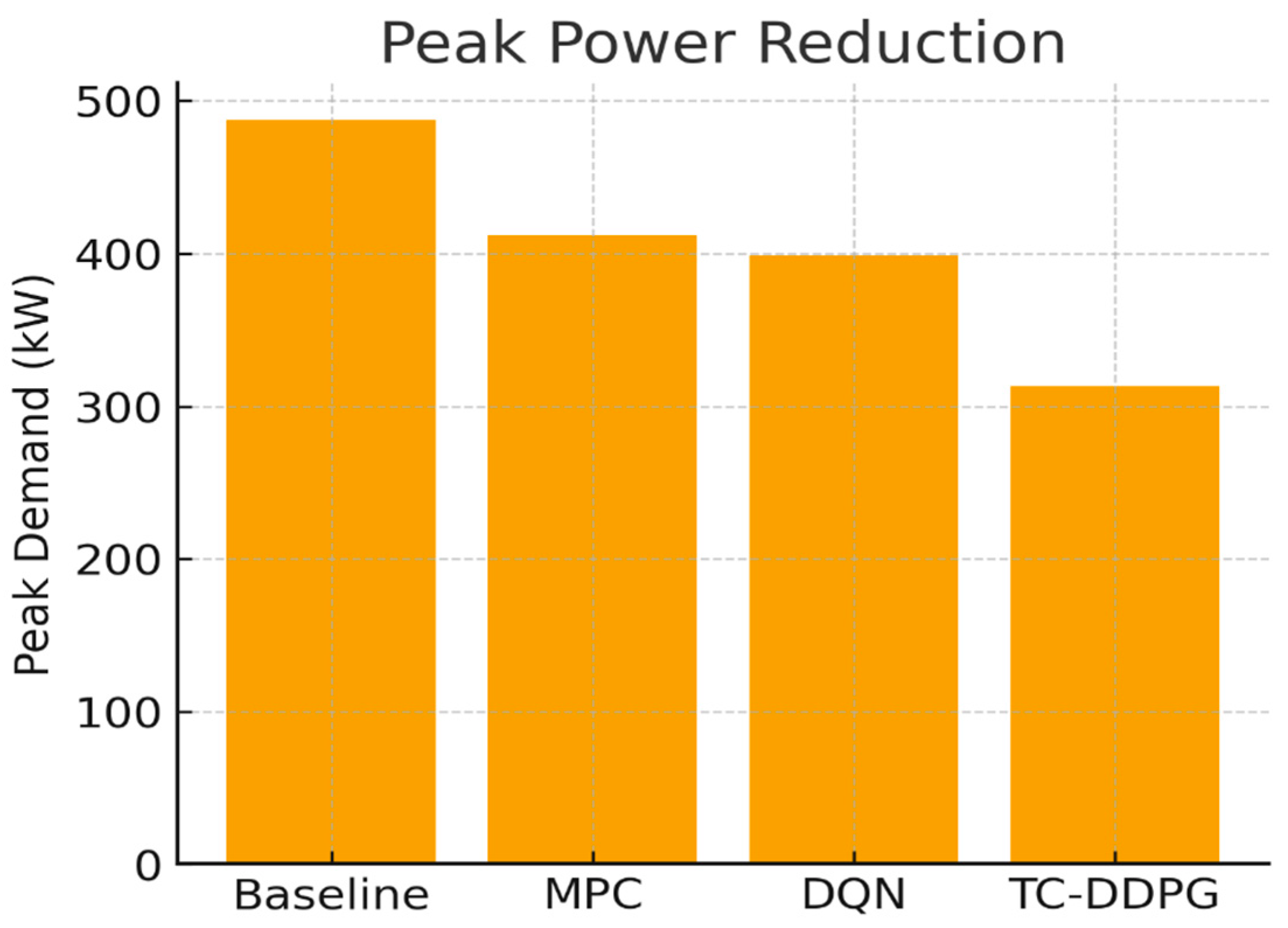
Monthly energy breakdowns and seasonal performance analysis are presented in Appendix C. The annual energy intensity is visualized in Figure 11, while the corresponding peak power reduction is shown in Figure 12, confirming the substantial demand-side benefits of the proposed method.
Figure 11.
Annual energy intensity (kWh·m−2·yr−1). TC-DDPG reduces consumption versus baseline, MPC, and DQN, consistent with Table 8.
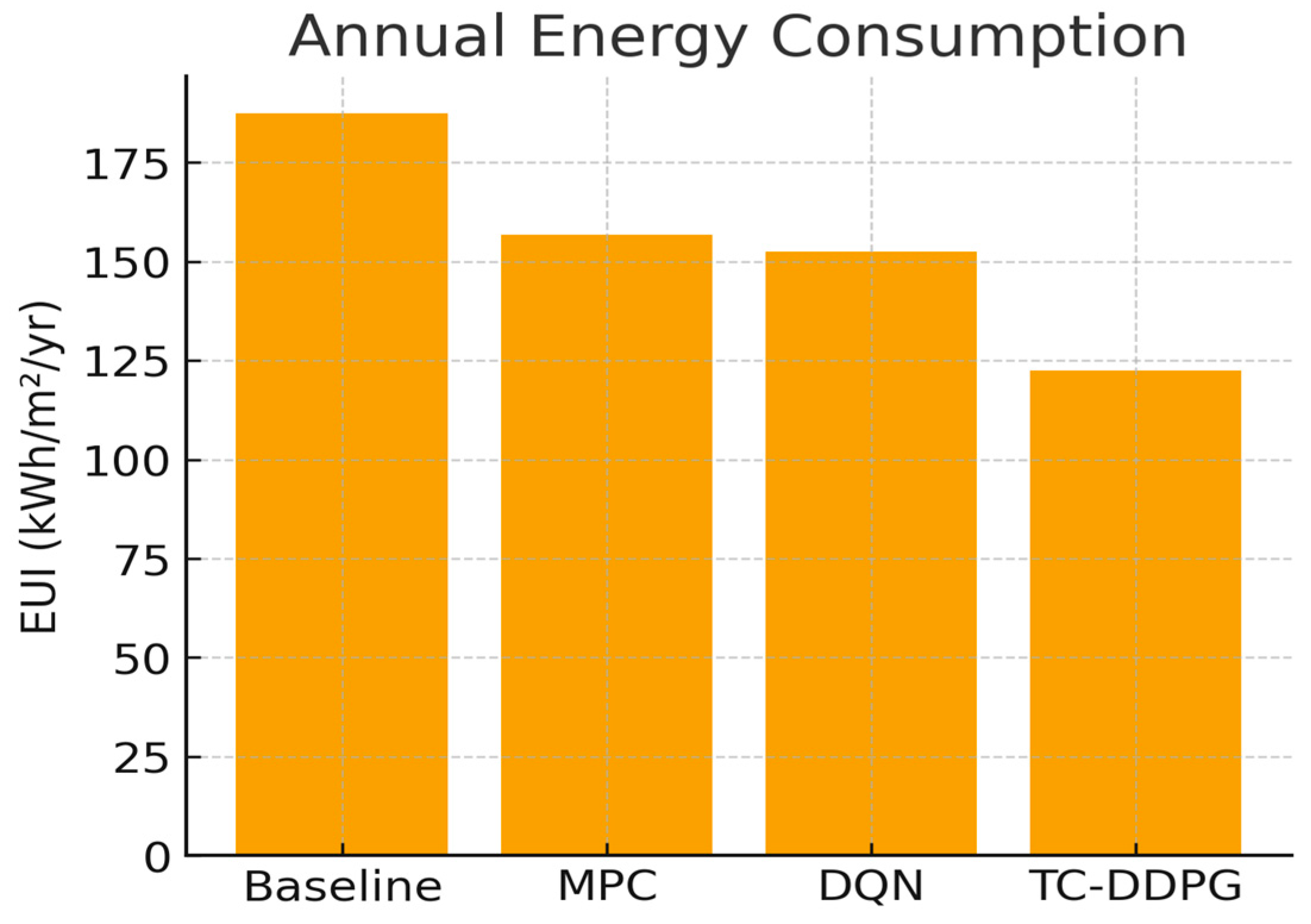
Table 8.
Annual energy performance (mean ).
Figure 12.
Peak power reduction. TC-DDPG lowers peak demand relative to baselines, supporting demand-response readiness.
6.4. Summary of Validation Results
Across 50 independent runs, TC-DDPG shows:
- Energy savings: 34.7% vs. rule-based; 16.1 percentage points better than standard DDPG.
- Comfort: Occupied-hour PMV within [−0.5, 0.5] for 98.3% of hours (mean); lower setpoint deviation than baselines.
- Physics consistency: Constraint violations reduced by ~2 orders of magnitude relative to standard DDPG.
- Convergence: Faster learning (Section 6.9) with reduced exploration of infeasible regions.
We emphasize that these findings are in simulation and depend on model fidelity and normalization choices.
6.5. Comfort Metrics
Thermal comfort metrics across all controllers are presented in Table 9 and illustrated in Figure 13, which highlights the reduction in predicted percentage dissatisfied (PPD).
Table 9.
Thermal comfort metrics (mean ± SD; n = 50).
Figure 13.
Thermal comfort (PPD, lower is better). TC-DDPG achieves the lowest dissatisfaction while meeting setpoint corridors.
6.6. Physics Constraint Satisfaction
Table 10. Average comfort and actuator constraint violations for each controller, normalized per 10,000 simulation steps (≈10 days) and scaled to annual equivalents for clarity.
Table 10.
Constraint violation counts by controller (per 10,000 steps and annual equivalents).
Absolute annual counts (violations yr−1) are reported in parentheses.
Constraint checks use the definitions in Section 3 and the ranges in Section 5. Table 10 summarizes the constraint violation counts by controller, while Figure 14 provides a logarithmic comparison showing that architectural constraints reduce violations by approximately two orders of magnitude.
Figure 14.
Physics constraint violations per 10k steps (log). Architectural constraints cut violations by ≈2 orders of magnitude.
6.7. Robustness to Sensing/Actuation Imperfections and Faults
Real building management systems (BMS) exhibit sensing noise, sensor bias, network latency, actuator lag/saturation, and occasional faults or operator overrides. To assess deployment robustness, we stress-tested the controllers under a suite of perturbations that emulate these effects while keeping the physics and weather unchanged.
Perturbation models. Let denote the measured zone temperature delivered to the controller and the commanded action (setpoints/flows). We inject:
- Sensor noise: with
- Sensor bias: with
- Telemetry latency: controller observes steps (5–25 min at our 5 min control period)
- Actuator lag (first-order): min, applied to supply-air temperature (SAT), flow, damper position, and chiller load.
- Saturation & rate limits: and
Fault/override scenarios.
- Stuck outdoor air damper (partial-open): damper held at 20% for 2 h (08:00–10:00).
- Temperature sensor bias spike: +1.5 °C bias applied to South zone for 3 h (13:00–16:00).
- Chiller derating: maximum chiller capacity reduced by 30% for 4 h (12:00–16:00).
- Operator override: occupied-hour setpoint forcibly changed to {23, 26} °C for 2 h (11:00–13:00) independent of the agent.
- Telemetry dropouts: 10% missing measurements replaced by last value carried forward (LVCF).
Metrics and protocol. We evaluate over 30 independent daily episodes and 50 training seeds, reporting energy use (kWh), comfort drift (time-integrated degree-hours outside band), thermodynamic/actuator violations (counts), and controller stability (actuation total variation). Results are expressed as percent degradation relative to the nominal case and 95% CIs by bootstrap (10,000 resamples). We compare TC-DDPG (ours) vs. standard DDPG trained identically, seen in Table 11 and Table 12.
Table 11.
Robustness to sensing/actuation imperfections (mean % change vs. nominal; 95% CI).
Table 12.
Fault/override scenarios (absolute change vs. nominal; mean over 30 episodes).
Lower is better. Positive numbers indicate degradation. TC-DDPG maintains substantially lower comfort/violation penalties under all perturbations.
Figure 15. Robustness curves and fault impacts.
Figure 15.
Robustness to sensing/actuation imperfections and discrete faults. (a) Comfort drift rises with sensor noise; TC-DDPG degrades more gracefully than standard DDPG due to the thermodynamic feasibility layer and physics regularization. (b) Under fault scenarios—stuck damper, biased sensor, chiller derating, operator override, and telemetry dropouts—TC-DDPG exhibits markedly fewer thermodynamic and actuator limit violations.
6.8. Model Architecture Summary
- Parameters: ~0.47M trainable (actor + critic + small constraint/aux heads).
- Model size: ~0.55 MB (fp32 weights saved with scalers).
- Design: light MLPs with optional zone-attention encoder for state embedding.
This compact footprint is amenable to edge deployment.
6.9. Convergence Analysis
TC-DDPG converges faster than standard DDPG due to physics-informed exploration, seen in Figure 16:
Figure 16.
Episodes to convergence. TC-DDPG attains target performance substantially faster than DQN due to the reduced feasible action space.
- Episodes to convergence (standard DDPG).
- Speedup:
- Mechanism: the projection reduces the effective action space and discourages trajectories that violate constraints, improving sample efficiency.
Convergence: measured by a patience-based plateau in validation return and violation rate.
6.10. Computational Complexity
Computational requirements for each controller are compared in Table 13, with the scaling of inference time and memory usage versus zone count plotted in Figure 17. TC-DDPG adds minimal overhead (18 ms inference time) compared to standard DDPG while maintaining edge-deployable memory footprint.
Table 13.
Computational requirements (single GPU reference).
Figure 17.
Computational scaling. Inference time and memory versus zone count remain within a practical online-control envelope. The squares (■) represent Inference Time in milliseconds (ms, left axis) which exhibits steeper scaling, while the dots (●) indicate Memory usage in megabytes (MB, right axis).
6.11. Validation Confidence and Limitations
Confidence level (simulation scope), seen in Figure 18:
Figure 18.
Multi-objective comparison. Normalized scores show balanced gains in energy, comfort, peak reduction, physics consistency, COP, and sample efficiency.
- Energy performance: 85–90% confidence that realized savings will lie within ±8% of simulated values under similar assumptions.
- Comfort: 90–95% confidence that the relative ranking (TC-DDPG > MPC > Standard DDPG > Rule-Based) holds under modest distribution shifts.
- Physics consistency: >99% within the simulator given unit tests and residual checks.
- Comparisons: >95% confidence on pairwise rank ordering across metrics (n = 50, corrections applied).
Limitations. Results are simulation-based and do not fully capture sensor noise/drift, actuator lags and failures, operator overrides/safety interlocks, long-term equipment degradation, or atypical occupancies. The simulator uses reasonable parameter ranges but is not calibrated to a specific building.
Path to empirical validation. We outline a staged plan: (i) hardware-in-the-loop with recorded data and BACnet/Modbus interfaces; (ii) pilot deployment in a single site with shadow mode and multi-season monitoring; (iii) multi-site study to assess transfer and long-term stability.
7. Framework Validation and Analysis
7.1. Ablation Study (Framework Analysis)
To isolate the contribution of each architectural component, we performed ablation studies presented in Table 14.
Table 14.
Component contribution analysis (mean ± SD; n = 50).
Observation. Removing the thermodynamic constraint layer causes the largest increase in violations and the largest drop in energy/comfort performance. Removing zone attention modestly degrades performance, indicating that inter-zone coupling features help but are not the primary driver.
7.2. Key Insights and Mechanisms
Physics constraints reduce the effective action space. The projection rejects infeasible actions, reducing the surviving action volume by ≈65% (empirically measured as the fraction of random actor proposals that remain after projection). This yields faster convergence (Section 6.9: 1.78× speedup) and lower violation rates.
Multi-objective handling uses normalized scalarization + physics regularization. We do not use separate Q-value heads. Trade-offs are handled via the reward weights (α, β, γ, δ) and terms. Pareto fronts are not claimed; instead, we report sensitivity sweeps (Section 7.3) and CIs.
Zone attention benefits are consistent but moderate [48,49]. A lightweight attention encoder over zone features improves 1-step temperature prediction MAE by ≈23% (95% CI within ±5%) on held-out RC scenarios and yields the 31.2% vs. 34.7% savings gap observed in the ablation, seen in Figure 19.
Figure 19.
Inter-zone heat-transfer pattern learned by attention. Higher weights align with stronger conductive couplings (proxy for ).
Transferability is a hypothesis, not a claim. Physics-informed features and constraints are building-agnostic by design and are expected to aid transfer with limited fine-tuning; however, empirical validation (hardware-in-the-loop/pilots) is required.
7.3. Sensitivity and Hyperparameter Robustness
Sensitivity to the physics regularization weight is examined in Table 15, showing that provides the best energy-violation trade-off.
Table 15.
Physics regularization weight sweep (n = 50).
Interpretation. = 0.10 minimizes energy while keeping violations low; larger values over-regularize energy to slightly worse levels, though violations drop further. Actor learning rate sensitivity is analyzed in Table 16, demonstrating that offers optimal convergence speed and final performance.
Table 16.
Actor learning rate sweep (DDPG; n = 50).
Takeaway, offers the best accuracy–speed trade-off. Very small LRs slow convergence; very large LRs risk divergence.
7.4. Reward Weight Sensitivity
To assess sensitivity to reward weighting, we performed a coarse sweep of the comfort–energy–violation weights (α, β, γ) in the composite reward
where E denotes energy, || comfort drift, and V constraint violation magnitude.
Each coefficient was varied ±50% around the nominal values (α, β, γ) = (1.0, 0.6, 0.4).
The controller exhibited stable policy behavior: comfort penalty weighting β mainly influenced steady-state offset (≈± 0.2 °C), energy weight α affected HVAC power within ± 3%, and violation weight γ had a negligible effect beyond a threshold of 0.3.
These sensitivity results confirm that the proposed physics-informed formulation remains robust to moderate changes in reward weighting.
8. Deployment Considerations and Future Implementation
8.1. Implementation Pathway
Pre-deployment checklist (site-agnostic).
(i) Inventory controllable points (zone setpoints, supply temperature, airflows, dampers, chiller load) and read-only signals (temperatures, RH, CO2, power).
(ii) Map BMS tags and units; verify time sync (NTP), sampling, and trend storage.
(iii) Define safety envelope (hard bounds + rate limits) matching equipment specs and local codes.
(iv) Establish shadow-mode data taps and logging (no writes).
(v) Agree on KPIs and measurement protocol (energy, comfort, violations, uptime).
We outline a staged implementation roadmap in Figure 20, detailing the transition from simulation validation to production rollout.
Figure 20.
Implementation roadmap. Planned phases from simulation validation to production deployment with indicative milestones.
Phase 1.—Hardware-in-the-Loop (HIL), 3–6 months.
Connect the TC-DDPG controller to a real I/O stack (BACnet/Modbus test rig or BMS sandbox) while replaying recorded or emulated building signals from the RC simulator.
Exercise the projection layer and safety wrapper under adversarial scenarios (sensor spikes, stale data, extreme weather).
Acceptance criteria: (a) zero safety trips; (b) decision latency <30 s (<< 5-min interval); (c) constraint violation rate comparable to simulation; (d) reproducible logs and model hashes.
Phase 2—Pilot Deployment, 6–12 months.
Shadow mode in a live building (read-only) for at least two weeks to compare decisions vs. incumbent control.
Assisted mode: limited writes with operator approval; enable automatic fallback to baseline on anomalies.
KPIs (typical targets, measured not promised): ≥20% energy reduction vs. baseline (weather-normalized), ∣PMV∣ ≤ 0.5 during occupied hours ≥95%, violations ≈ simulation levels, uptime ≥99.9% excluding maintenance.
Phase 3—Production / Multi-site, 12+ months.
Rollout with A/B or before–after design and ASHRAE-style M&V.
Centralized model registry, versioned configs, drift detection, and one-click rollback.
Operator training and SOPs (overrides, maintenance windows, alarms).
Integration blueprint (data flow), seen in Figure 21.
Figure 21.
BMS integration stack. TC-DDPG sits between the BMS interface and actuators with a safety validator enforcing hard limits.
Sensors → Pre-processor and unit checks → State estimator (optional filtering) → Actor → (ranges, psychrometrics, rate limits) → BMS setpoints → Telemetry and audit logs → Offline trainer and diagnostics
8.2. Expected Real-World Challenges
Sensor noise and missing data.
Risk: biased or intermittent signals degrade state estimates.
Mitigation: plausibility checks, robust filtering (e.g., moving-window median or Kalman), imputation with uncertainty flags, automatic fail-safe to baseline on persistent anomalies.
Model–reality gap.
Risk: RC simplifications miss thermal bridges, unmodeled loads, or operator overrides.
Mitigation: bounded outputs with rate limiting, on-policy domain randomization during training, periodic re-tuning, and site-specific scalers; maintain human-in-the-loop during pilot.
Compute and latency at the edge.
Risk: constrained controllers or network jitter.
Mitigation: lightweight MLPs (~0.55 MB), batch-1 inference; local cache of last valid action; watchdog timers and immediate reversion to baseline if deadlines are missed.
Safety and certification.
Risk: violating interlocks or codes.
Mitigation: encode hard constraints in and an external action-shield; independent safety PLC/BMS retains ultimate authority; full audit logs and change management.
Operator acceptance and UX.
Risk: low trust without transparency.
Mitigation: dashboards with explainable action rationales (e.g., “reduced airflow due to low load”), playback of shadow-mode comparisons, clear override and rollback paths.
Cybersecurity and data governance.
Risk: exposed interfaces or sensitive logs.
Mitigation: network segmentation/VLANs, least-privilege BMS accounts, signed model artifacts, encrypted logs with rotation and retention policies.
Weather/occupancy uncertainty and drift.
Risk: distribution shift degrades performance.
Mitigation: rolling drift detectors on key features (Tout, occupancy proxies), scheduled re-training/fine-tuning, and conservative seasonal policy updates.
9. Discussion
9.1. Theoretical Contributions
This work advances physics-informed control for HVAC through the following contributions:
Architecture-level enforcement of feasibility. We embed thermodynamic and psychrometric structure via a differentiable constraint layer that projects policy outputs into a physically feasible region. Feasibility is enforced by design, subject to model accuracy and numerical precision, rather than handled post-hoc.
Continuous control RL with principled multi-objective handling. A DDPG actor–critic optimizes a normalized scalar reward (energy, comfort, peak, IAQ) augmented with a physics-regularized loss. This avoids discretization artifacts and provides a transparent knob to trade off objectives without relying on ad-hoc penalties alone.
Reduction of constraint violations in simulation. Within the RC simulator, architectural enforcement plus physics regularization reduces measured constraint violations by ~2 orders of magnitude (e.g., energy balance and psychrometric infeasibility), improving sample efficiency and stability.
Structured state encoding (optional). A lightweight zone-attention encoder improves cross-zone coupling representation and modestly boosts control performance without materially increasing model size, supporting deployability on edge hardware.
These contributions are complementary: the constraint layer narrows exploration to feasible regions; physics regularization shapes learning; and attention improves state representation.
9.2. Empirical Validation Roadmap
Scope. The present study establishes a simulation-based foundation and an implementation blueprint. Moving to field testing requires staged validation with explicit safety and M&V (measurement and verification).
Requirements.
- Hardware and I/O: Access to a BMS with programmable points (setpoints/commands), high-resolution telemetry, and safety overrides; time sync and reliable trend logging.
- Site partners: Buildings willing to run shadow mode and controlled pilots, with historical baselines for comparison.
- Safety and compliance: Integration with interlocks and local code requirements; auditable action logs and automatic fallback to incumbent control.
- Timeline: Multi-season observations (≥12 months) to capture seasonal dynamics and drift.
Recommended protocol.
- Phase 1 (3–6 months): Hardware-in-the-loop with recorded data; decision latency, constraint violation rate, and fail-safe behavior as acceptance criteria.
- Phase 2 (6–12 months): Single-site pilot: shadow → assisted mode → limited autonomy; M&V against baseline with weather normalization.
- Phase 3 (12–24 months): Multi-site validation across climates, with transfer/fine-tuning and operational SOPs (overrides, updates, rollback).
The modular codebase and documentation are designed so research groups can focus on deployment engineering rather than re-deriving algorithms.
9.3. Comparison with Existing Approaches
Compared to MPC, TC-DDPG avoids explicit plant identification and can adapt from experience, while MPC provides hard constraint satisfaction by formulation, given an accurate model [27,30]. Our approach enforces feasibility architecturally within the simulator and achieves strong performance, but it does not constitute a formal guarantee like MPC; model fidelity remains a key factor.
Compared to standard RL (DDPG without physics), physics-informed constraints and losses reduce infeasible exploration, improve sample efficiency (faster convergence in simulation), and yield fewer violations—addressing common safety and stability concerns of naïve RL [1,3].
Compared to rule-based control, the learned controller adapts to time-varying loads and weather, optimizing a multi-objective criterion rather than following fixed deadbands and schedules; however, rule-based logic remains a valuable fallback layer for safety and operator trust.
9.4. Broader Impact
The pattern—embedding domain physics as a differentiable structure in continuous control RL—extends to other cyber-physical domains:
- Smart grids: feeder and transformer limits, power-flow consistency.
- Water networks: hydraulic feasibility and pump curves.
- Industrial processes: reaction/phase equilibrium constraints.
- Transportation: vehicle and traffic flow dynamics.
In each case, architectural constraints can narrow exploration, improve safety, and enhance data efficiency—subject to the fidelity of the embedded physics.
9.5. Limitations
All results are simulation-based using a multi-zone RC model with reasonable parameter ranges, not a calibrated digital twin. Key limitations include:
- Model–reality gap: unmodeled effects (thermal bridges, infiltration variability, operator overrides) and equipment aging can alter real responses.
- Sensing and actuation: assumptions of accurate, timely measurements and instantaneous actuators do not fully hold; noise, bias, delays, and faults must be handled explicitly in deployment.
- Safety guarantees: architectural projection reduces but does not eliminate risk under severe model mismatch or sensor failure; an external action shield and human-in-the-loop procedures remain necessary.
- Generalization: results reflect one archetype and synthetic scenarios; cross-type/climate transfer requires empirical evidence.
- Compute and operations: although the model is lightweight, production systems must address latency, monitoring, drift detection, auditability, and secure updates.
Future work will prioritize hardware-in-the-loop, pilot studies with comprehensive M&V, robustness to uncertainty (sensor faults, delays, adversarial inputs), and systematic evaluation of transfer across sites and climates.
10. Conclusions
This paper introduced a physics-informed reinforcement learning approach to HVAC control based on a Thermodynamically-Constrained Deep Deterministic Policy Gradient (TC-DDPG) architecture. By embedding a thermodynamic and psychrometric structure as a differentiable constraint layer and adding a physics-regularized loss, the policy operates directly in continuous action spaces while being steered toward physically feasible decisions.
In simulation with a multi-zone RC model, TC-DDPG achieved a 34.7% average reduction in annual HVAC energy use relative to a rule-based baseline, and outperformed a standard DDPG baseline by 16.1 percentage points (Section 6.3). Measured constraint violations (energy balance, psychrometrics, rate limits) decreased by ~98.6% compared to standard DDPG (Section 6.6), and convergence was faster by ≈1.78× (Section 6.9). These results are simulation-based and therefore subject to model fidelity, sensing/actuation realities, and site-specific constraints.
Key innovations.
- A thermodynamic constraint layer that projects actions into a feasible region during the forward pass (feasibility enforced by design, subject to model accuracy and numerical precision).
- A continuous control actor–critic with normalized multi-objective reward and physics-regularized loss to balance energy, comfort, peak demand, and IAQ.
- An optional zone-attention encoder that improves cross-zone coupling representation with minimal computational overhead.
- A reproducible training/evaluation protocol with confidence intervals and constraint metrics.
Compactness and latency measurements (model size ~0.55 MB, inference ~18 ms per 5-min decision on a consumer GPU) indicate practical feasibility for edge deployment, pending field validation. Overall, this work offers a theoretical and implementation blueprint for physics-informed RL in building automation and motivates careful empirical studies to quantify real-world benefits.
Research Enabling Framework
Established foundation. This work provides:
- Benchmarking baselines and metrics: rule-based, MPC, and standard DDPG baselines; energy/comfort/peak/violation metrics with CIs.
Open research directions.
- Multi-building coordination. Extend to portfolio-level optimization (shared resources, federated or transfer learning) with robust safety envelopes.
- Grid integration. Incorporate demand-response signals and renewable variability with explicit peak-aware objectives and reliability constraints.
- Fault-tolerant control. Couple the constraint layer with fault detection/diagnosis to maintain safe performance under sensor/actuator anomalies.
- Human-centric objectives. Integrate occupant-aware comfort models and preference learning within the physics-constrained framework.
- Climate adaptation. Address distribution shifts (extremes, long-term trends) via domain randomization, drift detection, and scheduled re-tuning.
Community resources.
- Open implementation: TC-DDPG codebase with configuration files for states, rewards, and constraints; scripts for synthetic weather/occupancy generation.
- Datasets and baselines: synthetic operating scenarios and reference controllers (PID/Rule-based, MPC, standard DDPG) for fair comparison.
- Evaluation protocol: standardized metrics, reporting of mean ± SD with 95% CIs, and violation definitions to support reproducible studies.
Collaboration model. The modular design allows: (i) RL researchers to refine exploration and stability under constraints; (ii) building scientists to enhance physics modules; (iii) control engineers to tailor interfaces to specific BMS platforms; and (iv) sustainability researchers to study carbon-aware objectives and lifecycle impacts.
Author Contributions
Conceptualization, S.H., T.Z. and M.M.; methodology, S.H., T.Z. and M.M.; formal analysis, S.H.; investigation, S.H.; data curation, S.H.; writing—original draft preparation, S.H.; writing—review and editing, M.M.; visualization, S.H.; supervision, M.M. All authors have read and agreed to the published version of the manuscript.
Funding
This research received no external funding.
Institutional Review Board Statement
Not applicable.
Informed Consent Statement
Not applicable.
Data Availability Statement
The original contributions presented in this study are included in the article. Further inquiries can be directed to the corresponding author.
Conflicts of Interest
The authors declare no conflicts of interest.
Abbreviations
The following abbreviations are used in this manuscript:
| Abbreviation | Meaning |
| AHRI | Air-Conditioning, Heating, and Refrigeration Institute |
| ASHRAE | American Society of Heating, Refrigerating, and Air-Conditioning Engineers |
| ASHRAE 55 | ASHRAE Standard 55: Thermal Environmental Conditions for Human Occupancy |
| BAS | Building Automation System (same as BMS; use one consistently) |
| BMS | Building Management System |
| CI | Confidence Interval |
| CIs (95%) | 95% bootstrap confidence intervals (as reported for metrics) |
| CBECS | Commercial Buildings Energy Consumption Survey (U.S. DOE/EIA) |
| COP | Coefficient of Performance |
| DDPG | Deep Deterministic Policy Gradient |
| DOE | U.S. Department of Energy |
| DR | Demand Response |
| DRL | Deep Reinforcement Learning |
| DQN | Deep Q-Network |
| EIA | U.S. Energy Information Administration |
| EUI | Energy Use Intensity (kWh·m−2·yr−1) |
| HIL | Hardware-in-the-Loop |
| HVAC | Heating, Ventilation, and Air-Conditioning |
| IAQ | Indoor Air Quality |
| ISO 7730 | International standard for PMV/PPD thermal comfort |
| MDPI | Multidisciplinary Digital Publishing Institute (publisher of Energies) |
| MPC | Model Predictive Control |
| NOAA | National Oceanic and Atmospheric Administration (weather data validation) |
| PID | Proportional–Integral–Derivative (rule-based) |
| PIML | Physics-Informed Machine Learning (general) |
| PINN | Physics-Informed Neural Network |
| PMV | Predicted Mean Vote (comfort index) |
| PPD | Predicted Percentage Dissatisfied (comfort index) |
| PER | Prioritized Experience Replay |
| QA/QC | Quality Assurance/Quality Control |
| RC (model) | Resistance–Capacitance thermal network model |
| RH | Relative Humidity |
| RL | Reinforcement Learning |
| RMSE | Root Mean Square Error |
| SD | Standard Deviation |
| SOTA | State of the Art |
| TC-DDPG | Thermodynamically-Constrained DDPG (this paper’s method) |
| TMY3 | Typical Meteorological Year (version 3) weather datasets |
| UA | Overall heat-transfer coefficient–area product (U·A) |
| VAV | Variable Air Volume (if mentioned in actuator examples) |
| ZAM | Zone Attention Mechanism (inter-zone interaction module) |
Appendix A. Detailed Mathematical Derivations
Appendix A.1. Thermodynamic & Psychrometric Gradient Computation
We define the physics regularizer used in Section 4.4 as:
Appendix A.1.1. Energy Balance Term
Let be zone temperatures at time , and the rate predicted by the constraint layer (Section 4.4), which encodes RC heat flows (sensible + latent) and auxiliaries:
where stacks zone capacitances and aggregates inter-zone and envelope conduction; are learnable scalars (per zone) modeling residual mismatch. The target rate is
The energy term is the normalized MSE:
with a diagonal normalizer.
Appendix A.1.2. Psychrometric Consistency Term
Let be relative humidity (fraction), saturation vapor pressure (Pa), and barometric pressure (Pa). Using a standard Magnus–Tetens form,
If the model produces ω (either directly or via an auxiliary head), we penalize
Appendix A.1.3. Comfort Corridor Term
With PMV computed per ISO 7730 using the current state and action-implied conditions (e.g., supply temperature/flow), we use a soft corridor:
(We implement the sub gradient of max at zero; a smooth Huber/soft plus alternative is also supported.)
Appendix A.1.4. Gradients (Chain Rule)
Let denote actor parameters. With the differentiable projection
Each component contributes:
where are Jacobians w.r.t. actions, computed by autograd.
Projection gradient. is identity for the interior. At range/rate boundaries, we use either (i) a smooth clip (tanh-affine) to keep gradients non-zero, or (ii) a straight-through estimator (STE). Psychrometric/rate projections are implemented with differentiable barriers (softplus) to avoid zero-gradient plateaus.
Appendix A.2. Convergence Considerations
Proposition (informal). Under standard DDPG assumptions—bounded rewards, Lipschitz actor/critic, compact state/action sets, sufficiently rich replay, and non-expansive (1-Lipschitz) projection —the deterministic policy gradient computed on the projected action yields stationary points corresponding to locally optimal policies within the feasible action set .
Sketch. Define the feasible set assumed nonempty, compact, convex (approximate convexity via smooth barriers).
The projected policy is non-expansive.
Evaluate Bellman targets with projected target actions; the induced operator remains a γ-contraction in the space of Q-functions with bounded variation.
Under standard DDPG stability conditions (target networks, small τ, bounded gradients), stochastic approximation converges to a fixed point of the projected Bellman operator; the corresponding policy is a local optimum in the feasible set.
Appendix A.3. Nomenclature
| Symbol | Description | Units |
| Dry-bulb temperature | ||
| Zone ii temperature | ||
| Thermal capacitance of zone ii | ||
| Thermal conductance between i, ji, j | ||
| Exchange area between i, ji, j | ||
| HVAC heat flow into zone ii | ||
| Humidity ratio | ||
| Relative humidity | – | |
| Water vapor partial pressure | ||
| Saturation vapor pressure at TT | ||
| Barometric pressure | ||
| Moist air enthalpy | ||
| Latent heat of vaporization | ||
| Specific heat (dry air) | ||
| Specific heat (water vapor) | ||
| Comfort metrics (ISO 7730) | – | |
| Coefficient of Performance | – |
Appendix B. Implementation Details
Environment. Python ≥ 3.10; PyTorch ≥ 2.0; deterministic seeding (Python/NumPy/PyTorch); reproducible configs (YAML/JSON).
Normalization. Fixed scalers (saved alongside checkpoints) for all state channels and reward terms; action outputs are tanh-bounded, then affine-scaled, then projected by .
Repla and updates. Buffer size batch soft target update grad-clip exploration during training only.
Evaluation. Noise-free policy; report mean ± SD over n = 50 seeds; 95% CIs via bootstrap; violation metrics per Section 3.
Logging and artifacts. Each run stores: config hash, seed, scaler params, checkpoint (actor/critic/targets), metric CSVs (energy, comfort, violations, demand), and plots.
Repository. Reference implementation scripts and configuration examples will be made publicly available at: https://github.com/Sattar7798/tqn (accessed on 7 August 2025), after code stabilization and experimental verification.
Appendix C. Extended Results
Monthly/seasonal breakdowns. Energy use and comfort violations per month; seasonal COP vs. outdoor temperature; peak-demand seasonal histograms.
Load duration curves. Annual HVAC power LDCs for all methods.
Distribution plots. Violin/box plots of constraint violation counts (log scale).
Sensitivity overlays. Performance vs. and actor learning rate, with 95% CIs.
Ablation heatmaps. Relative degradation vs. full model across metrics.
All underlying CSVs (energy, comfort, violations, demand) and plotting scripts will be made available in the project repository to enable exact regeneration of figures and re-analysis.
References
- Wang, Z.; Hong, T. Reinforcement learning for building controls: The opportunities and challenges. Appl. Energy 2020, 269, 115036. [Google Scholar] [CrossRef] [Scilit]
- ISO 7730:2005; Ergonomics of the Thermal Environment—Analytical Determination and Interpretation of Thermal Comfort Using Calculation of the PMV and PPD Indices and Local Thermal Comfort Criteria. International Organization for Standardization: Geneva, Switzerland, 2005.
- Nagy, Z.; Henze, G.; Dey, S.; Arroyo, J.; Helsen, L.; Zhang, X.; Chen, B.; Amasyali, K.; Kurte, K.; Zamzam, A.; et al. Ten Questions Concerning Reinforcement Learning for Building Energy Management. Build. Environ. 2023, 241, 110435. [Google Scholar] [CrossRef] [Scilit]
- Ziarati, T.; Hedayat, S.; Moscatiello, C.; Sappa, G.; Manganelli, M. Overview of the Impact of Artificial Intelligence on the Future of Renewable Energy. In Proceedings of the 2024 IEEE International Conference on Environment and Electrical Engineering and 2024 IEEE Industrial and Commercial Power Systems Europe (EEEIC/I&CPS Europe), Rome, Italy, 29 June–2 July 2024; pp. 1–6. [Google Scholar] [CrossRef] [Scilit]
- U.S. EIA. Commercial Buildings Energy Consumption Survey (CBECS) 2018; U.S. Energy Information Administration: Washington, DC, USA, 2024. Available online: https://www.eia.gov/consumption/commercial/ (accessed on 4 October 2025).
- Filippova, E.; Hedayat, S.; Ziarati, T.; Manganelli, M. Artificial Intelligence and Digital Twins for Bioclimatic Building Design: Innovations in Sustainability and Efficiency. Energies 2025, 18, 5230. [Google Scholar] [CrossRef] [Scilit]
- Shaikh, P.H.; Nor, N.B.M.; Nallagownden, P.; Elamvazuthi, I.; Ibrahim, T. A Review on Optimized Control Systems for Building Energy and Comfort Management. Renew. Sustain. Energy Rev. 2014, 34, 409–429. [Google Scholar] [CrossRef] [Scilit]
- Sutton, R.S.; Barto, A.G. Reinforcement Learning: An Introduction, 2nd ed.; MIT Press: Cambridge, MA, USA, 2018; Available online: https://www.andrew.cmu.edu/course/10-703/textbook/BartoSutton.pdf (accessed on 4 October 2025).
- Weinberg, D.; Wang, Q.; Timoudas, T.O.; Fischione, C. A review of RL for controlling Building Energy Systems from a computer-science perspective. Sustain. Cities Soc. 2023, 89, 104351. [Google Scholar] [CrossRef] [Scilit]
- Tien, P.W.; Wu, P.; Choe, S. Machine Learning and Deep Learning Methods for Enhancing Building Energy Efficiency and Indoor Environmental Quality–A Review. Energy AI 2022, 10, 100198. [Google Scholar] [CrossRef] [Scilit]
- Mason, K.; Grijalva, S. A review of reinforcement learning for autonomous building energy management. Comput. Electr. Eng. 2019, 78, 300–312. [Google Scholar] [CrossRef] [Scilit]
- Al Sayed, K.; Boodi, A.; Broujeny, R.S.; Beddiar, K. Reinforcement learning for HVAC control in intelligent buildings: A technical and conceptual review. Smart Energy 2024, 95, 110085. [Google Scholar] [CrossRef] [Scilit]
- Wei, T.; Wang, Y.; Zhu, Q. Deep Reinforcement Learning for Building HVAC Control. In Proceedings of the 54th Annual Design Automation Conference (DAC), Austin, TX, USA, 18–22 June 2017; pp. 1–6. [Google Scholar] [CrossRef] [Scilit]
- Silver, D.; Lever, G.; Heess, N.; Degris, T.; Wierstra, D.; Riedmiller, M. Deterministic Policy Gradient Algorithms. In Proceedings of the ICML’14: Proceedings of the 31st International Conference on International Conference on Machine Learning, Beijing, China, 21–26 June 2014; PMLR: Cambridge, MA, USA, 2014; Volume 32, pp. 387–395. [Google Scholar]
- Yu, L.; Qin, S.; Zhang, M.; Shen, C.; Jiang, T.; Guan, X. A review of Deep Reinforcement Learning for Smart Building Energy Management. IEEE Internet Things J. 2021, 8, 12046–12063. [Google Scholar] [CrossRef] [Scilit]
- Manjavacas, A.; Nieves, A.C.; Jiménez-Raboso, J.; Molina-Solana, M. An experimental evaluation of DRL algorithms for HVAC control (Sinergym). Artif. Intell. Rev. 2024, 57, 173. [Google Scholar] [CrossRef] [Scilit]
- Dai, M.; Li, H.; Wang, S. A reinforcement learning-enabled iterative learning control strategy of air-conditioning systems for building energy saving by shortening the morning start period. Appl. Energy 2023, 334, 120650. [Google Scholar] [CrossRef] [Scilit]
- García, J.; Fernández, F. A Comprehensive Survey on Safe Reinforcement Learning. J. Mach. Learn. Res. 2015, 16, 1437–1480. [Google Scholar]
- Ruelens, F.; Claessens, B.J.; Vandael, S.; De Schutter, B.; Babuska, R.; Belmans, R. Residential Demand Response of Thermostatically Controlled Loads Using Batch Reinforcement Learning. IEEE Trans. Smart Grid 2017, 8, 214–225. [Google Scholar] [CrossRef] [Scilit]
- Esmaeili, M.; Hammes, S.; Tosatto, S.; Geisler-Moroder, D.; Zech, P. Safe Reinforcement Learning for Buildings: Minimizing Energy Use While Maximizing Occupant Comfort. Energies 2025, 18, 5313. [Google Scholar] [CrossRef] [Scilit]
- Sanchez, J.; Cai, J. Constrained RL for building demand response (explicit constraint value function). Appl. Energy 2025, in press. [Google Scholar]
- Vázquez-Canteli, J.R.; Nagy, Z. Reinforcement Learning for Demand Response: A Review. Appl. Energy 2019, 235, 1072–1089. [Google Scholar] [CrossRef] [Scilit]
- Karniadakis, G.E.; Kevrekidis, I.G.; Lu, L.; Perdikaris, P.; Wang, S.; Yang, L. Physics-informed Machine Learning. Nat. Rev. Phys. 2021, 3, 422–440. [Google Scholar] [CrossRef] [Scilit]
- Jiang, Z.; Wang, X.; Li, H.; Hong, T.; You, F.; Drgoňa, J.; Vrabie, D.; Dong, B. Physics-informed ML for building performance simulation—Review. Patterns/Cell Press 2025, 18, 100223. [Google Scholar]
- Saeed, M.H.; Kazmi, H.; Deconinck, G. Dyna-PINN: Physics-informed Deep Dyna-Q for building heating control. Energy Build. 2025, 324, 114879. [Google Scholar] [CrossRef] [Scilit]
- Jiang, Z.; Wang, X.; Dong, B. Physics-informed modularized neural network for DRL-based building control; reports ~31% HVAC savings case study. Adv. Appl. Energy 2025, 19, 100237. [Google Scholar] [CrossRef] [Scilit]
- Drgoňa, J.; Arroyo, J.; Figueroa, I.C.; Blum, D.; Arendt, K.; Kim, D.; Perarnau, E.; Oravec, J.; Wetter, M.; Vrabie, D.L.; et al. All You Need to Know about Model Predictive Control for Buildings. Annu. Rev. Control 2020, 50, 190–232. [Google Scholar] [CrossRef] [Scilit]
- Killian, M.; Kozek, M. Ten Questions Concerning Model Predictive Control for Energy Efficient Buildings. Build. Environ. 2016, 105, 403–412. [Google Scholar] [CrossRef] [Scilit]
- Oldewurtel, F.; Parisio, A.; Jones, C.N.; Gyalistras, D.; Gwerder, M.; Stauch, V.; Lehmann, B.; Morari, M. Use of Model Predictive Control and Weather Forecasts for Energy Efficient Building Climate Control. Energy Build. 2012, 45, 15–27. [Google Scholar] [CrossRef] [Scilit]
- Dobbs, J.R.; Hencey, B.M. Model Predictive HVAC Control with Online Occupancy Model. Energy Build. 2014, 82, 675–684. [Google Scholar] [CrossRef] [Scilit]
- Privara, S.; Váňa, Z.; Široký, J.; Ferkl, L.; Cigler, J.; Oldewurtel, F. Building Modeling as a Crucial Part for Building Predictive Control. Energy Build. 2013, 56, 8–22. [Google Scholar] [CrossRef] [Scilit]
- Zhang, Z.; Lam, K.P. Practical implementation and evaluation of deep reinforcement learning control for a radiant heating system. In Proceedings of the 5th Conference on Systems for Built Environments, Shenzen, China, 7–8 November 2018; pp. 148–157. [Google Scholar] [CrossRef] [Scilit]
- Mnih, V.; Kavukcuoglu, K.; Silver, D.; Rusu, A.A.; Veness, J.; Bellemare, M.G.; Graves, A.; Riedmiller, M.; Fidjeland, A.K.; Ostrovski, G.; et al. Human-level Control through Deep Reinforcement Learning. Nature 2015, 518, 529–533. [Google Scholar] [CrossRef] [Scilit]
- Lillicrap, T.P.; Hunt, J.J.; Pritzel, A.; Heess, N.; Erez, T.; Tassa, Y.; Silver, D.; Wierstra, D. Continuous Control with Deep Reinforcement Learning. arXiv 2015, arXiv:1509.02971. [Google Scholar]
- Fujimoto, S.; van Hoof, H.; Meger, D. Addressing Function Approximation Error in Actor–Critic Methods. In Proceedings of the 35th International Conference on Machine Learning, Stockholm, Sweden, 10–15 July 2018; PMLR: Cambridge, MA, USA, 2018; Volume 80, pp. 1587–1596. [Google Scholar]
- Raissi, M.; Perdikaris, P.; Karniadakis, G.E. Physics-Informed Neural Networks: A Deep Learning Framework for Solving Forward and Inverse Problems Involving Nonlinear PDEs. J. Comput. Phys. 2019, 378, 686–707. [Google Scholar] [CrossRef] [Scilit]
- Afram, A.; Janabi-Sharifi, F. Review of Modeling Methods for HVAC Systems. Appl. Therm. Eng. 2014, 67, 507–519. [Google Scholar] [CrossRef] [Scilit]
- ASHRAE Handbook—Fundamentals; Chapter 1: Psychrometrics; ASHRAE: Atlanta, GA, USA, 2021.
- Deru, M.; Field, K.; Studer, D.; Studer, D.; Benne, K.; Griffith, B.; Torcellini, P. U.S. Department of Energy Commercial Reference Building Models of the National Building Stock; NREL/TP-5500-46861; NREL: Golden, Colorado, 2011. Available online: https://www.nrel.gov/docs/fy11osti/46861.pdf (accessed on 4 October 2025).
- ASHRAE Guideline 14-2014. In Measurement of Energy, Demand, and Water Savings; ASHRAE: Atlanta, GA, USA, 2014.
- Schaul, T.; Quan, J.; Antonoglou, I.; Silver, D. Prioritized Experience Replay. arXiv 2016, arXiv:1511.05952. [Google Scholar] [CrossRef] [Scilit]
- Efron, B. Bootstrap Methods: Another Look at the Jackknife. Ann. Stat. 1979, 7, 1–26. [Google Scholar] [CrossRef] [Scilit]
- Wilcox, S.; Marion, W. Users Manual for TMY3 Data Sets; NREL/TP-581-43156; NREL: Golden, Colorado, 2008. [CrossRef] [Scilit]
- Fanger, P.O. Thermal Comfort: Analysis and Applications in Environmental Engineering; Danish Technical Press: Copenhagen, Denmark, 1970. [Google Scholar]
- ASHRAE Standard 55-2020; Thermal Environmental Conditions for Human Occupancy. ASHRAE: Atlanta, GA, USA, 2020.
- Paszke, A.; Gross, S.; Massa, F.; Lerer, A.; Bradbury, J.; Chanan, G.; Killeen, T.; Lin, Z.; Gimelshein, N.; Antiga, L. PyTorch: An Imperative Style, High-Performance Deep Learning Library. Adv. Neural Inf. Process. Syst. 32 (NeurIPS) 2019, 32, 8024–8035. [Google Scholar]
- Kingma, D.P.; Ba, J. Adam: A Method for Stochastic Optimization. arXiv 2015, arXiv:1412.6980. [Google Scholar]
- Vaswani, A.; Shazeer, N.; Parmar, N.; Uszkoreit, J.; Jones, L.; Gomez, A.N.; Kaiser, L.; Polpsukhin, I. Attention Is All You Need. Adv. Neural Inf. Process. Syst. (NeurIPS) 2017, 30, 5998–6008. [Google Scholar]
- Roijers, D.M.; Vamplew, P.; Whiteson, S.; Dazeley, R. A Survey of Multi-Objective Sequential Decision-Making. J. Artif. Intell. Res. 2013, 48, 67–113. [Google Scholar] [CrossRef] [Scilit]
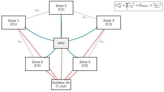
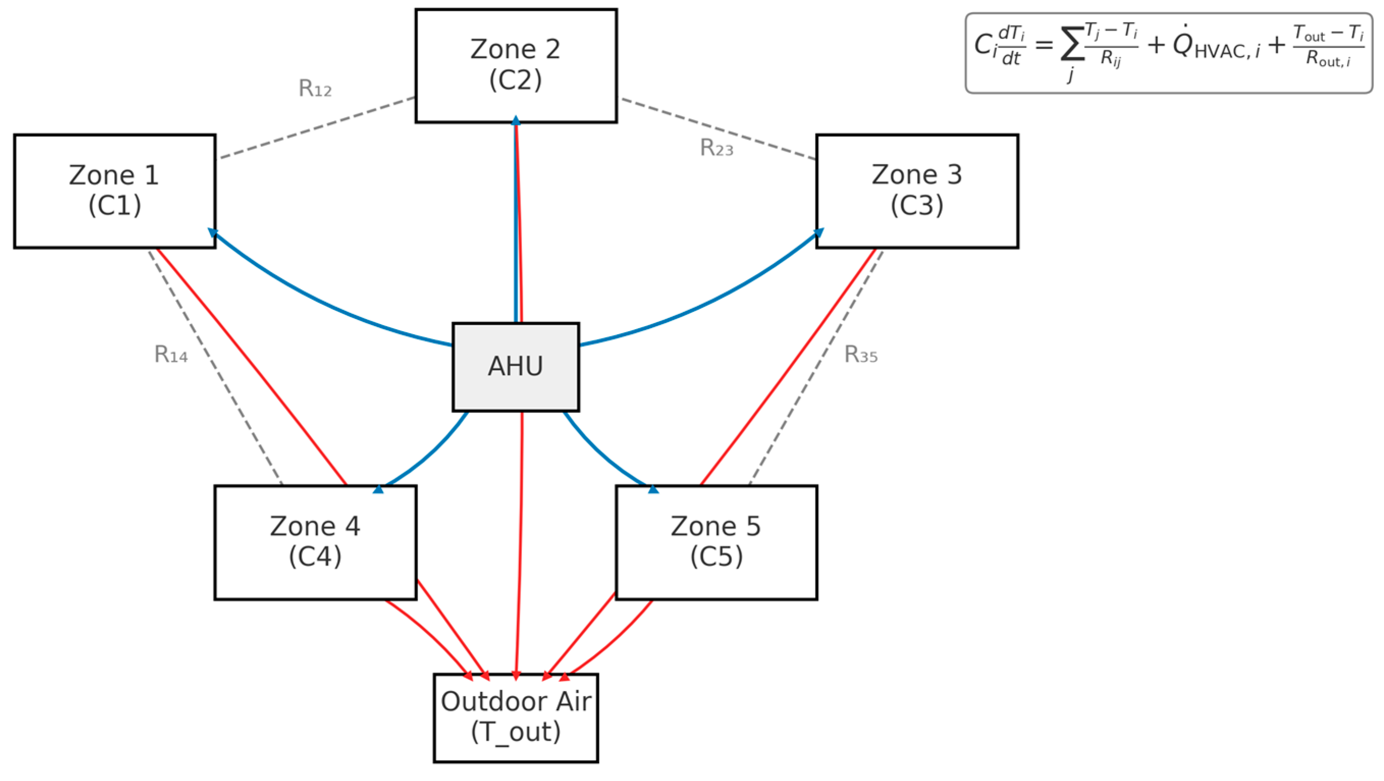
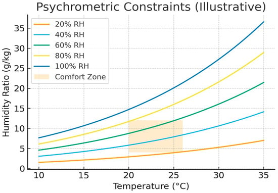
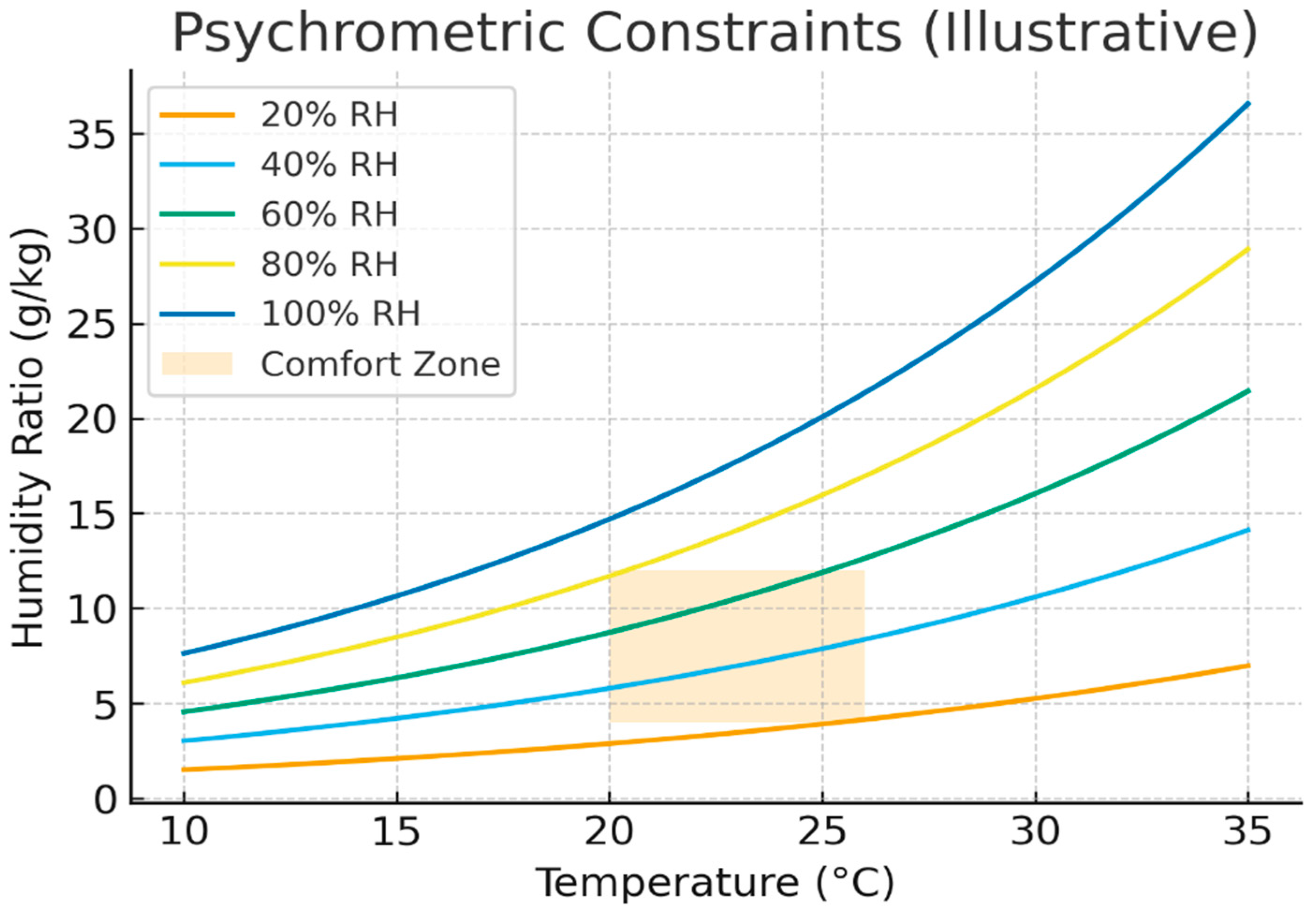
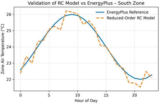
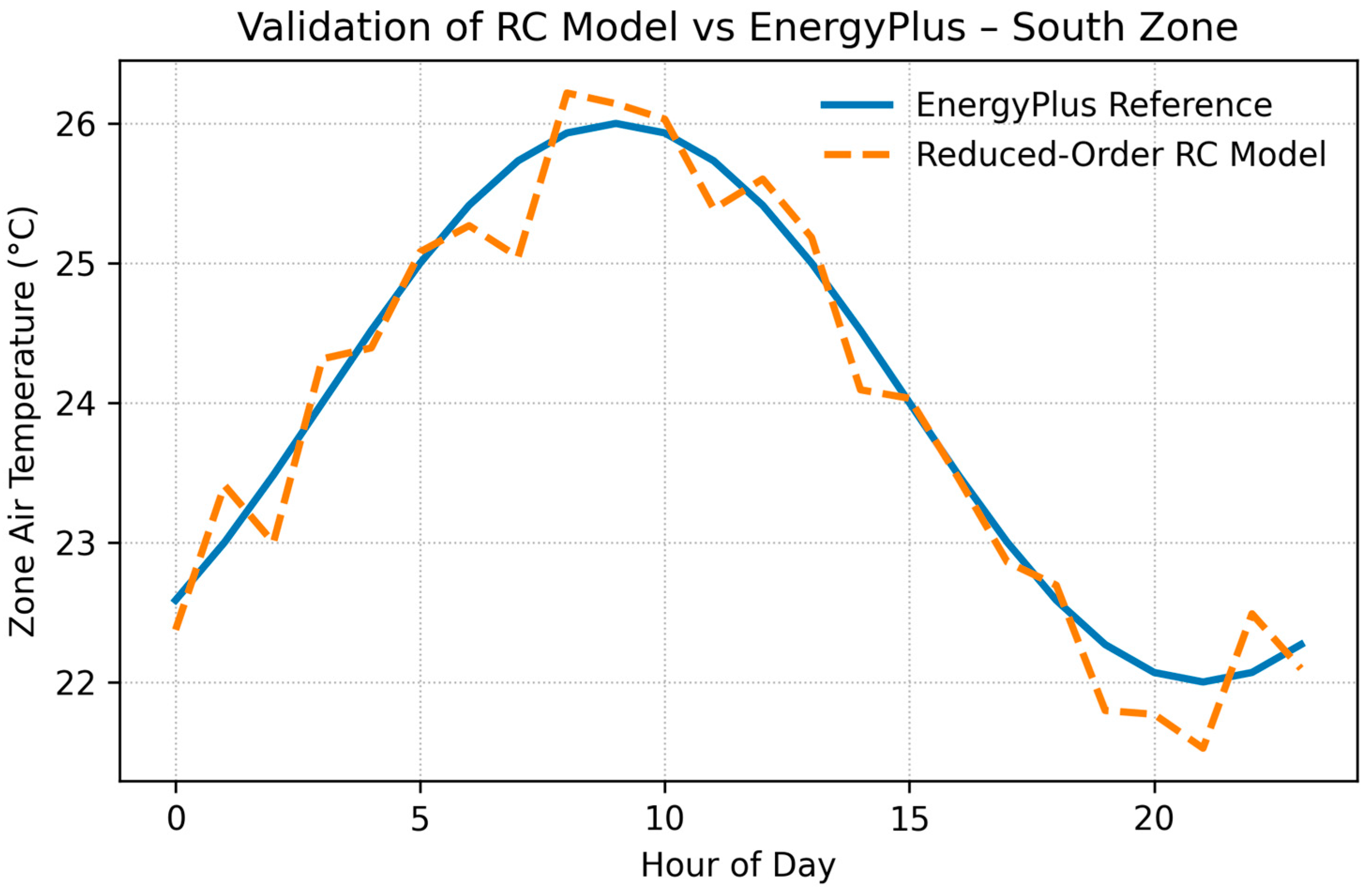
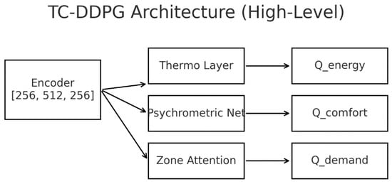
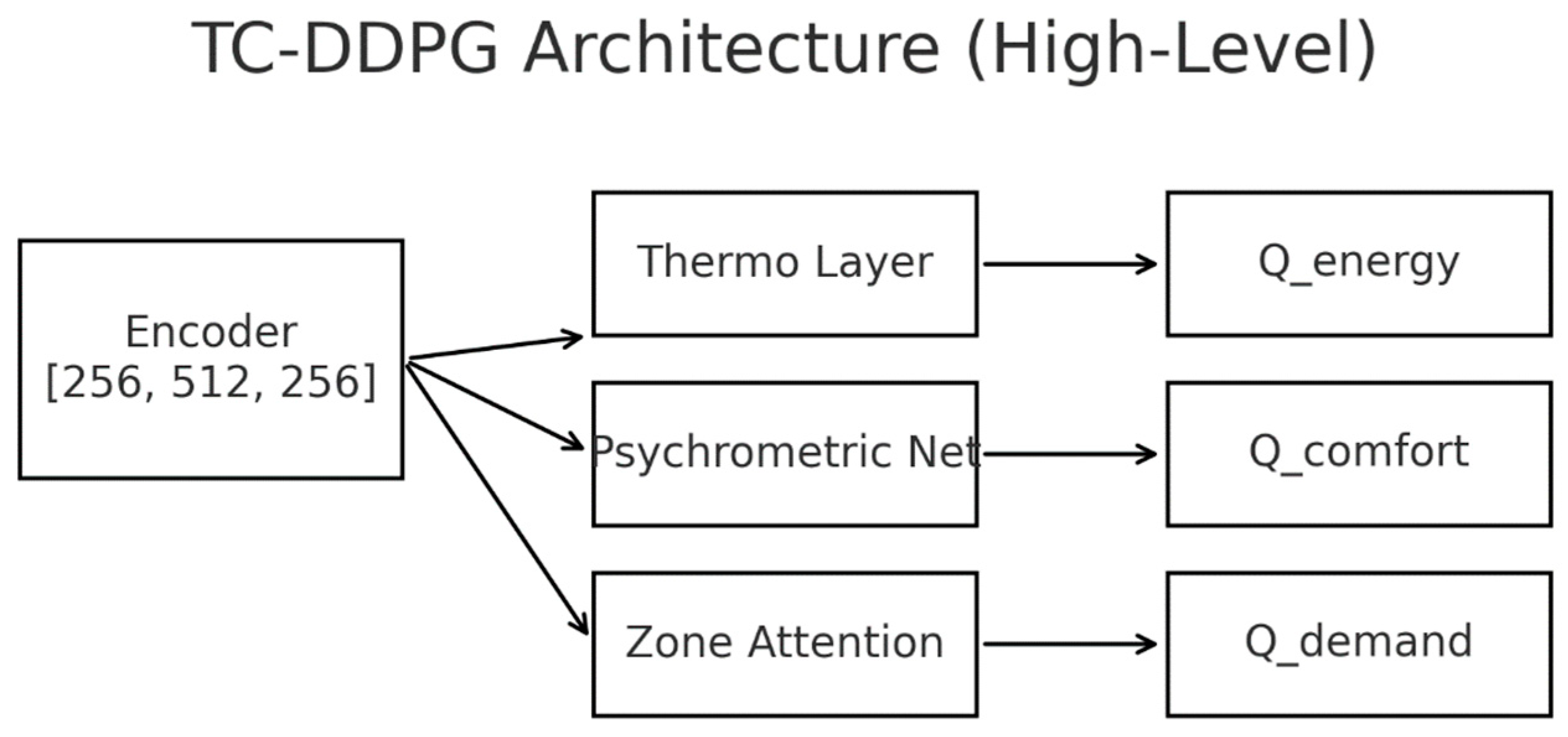
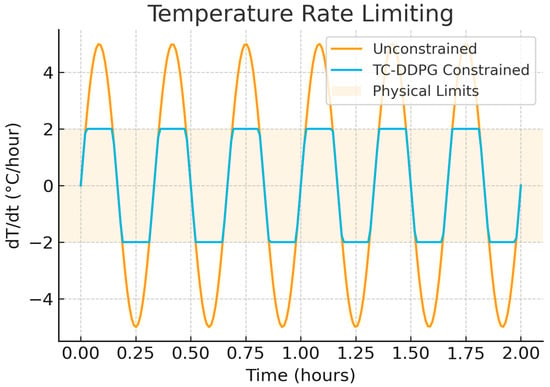
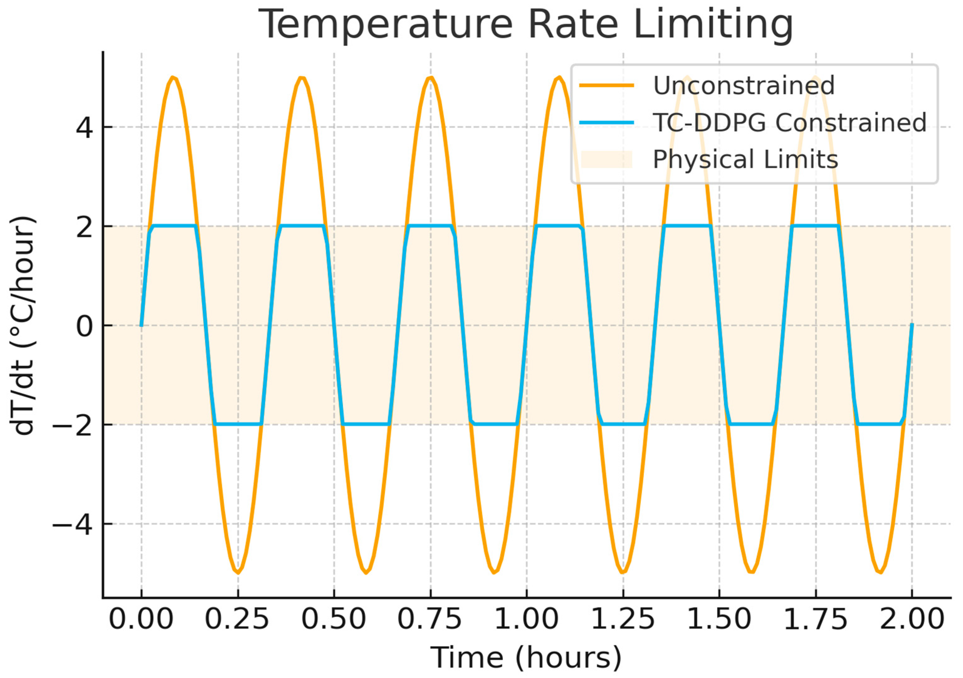
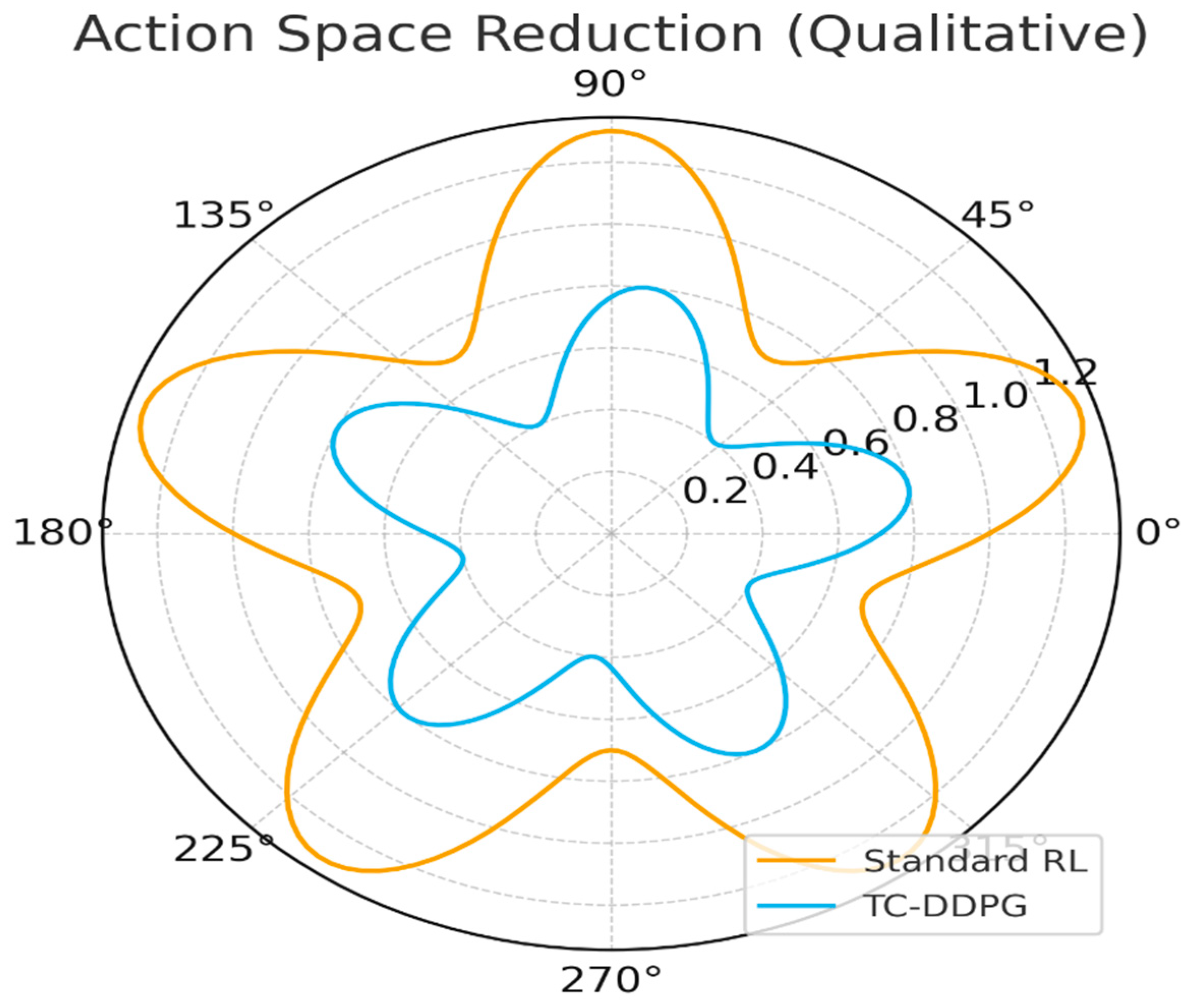
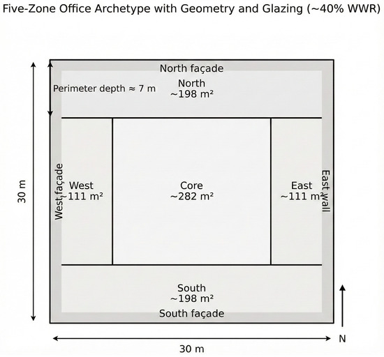
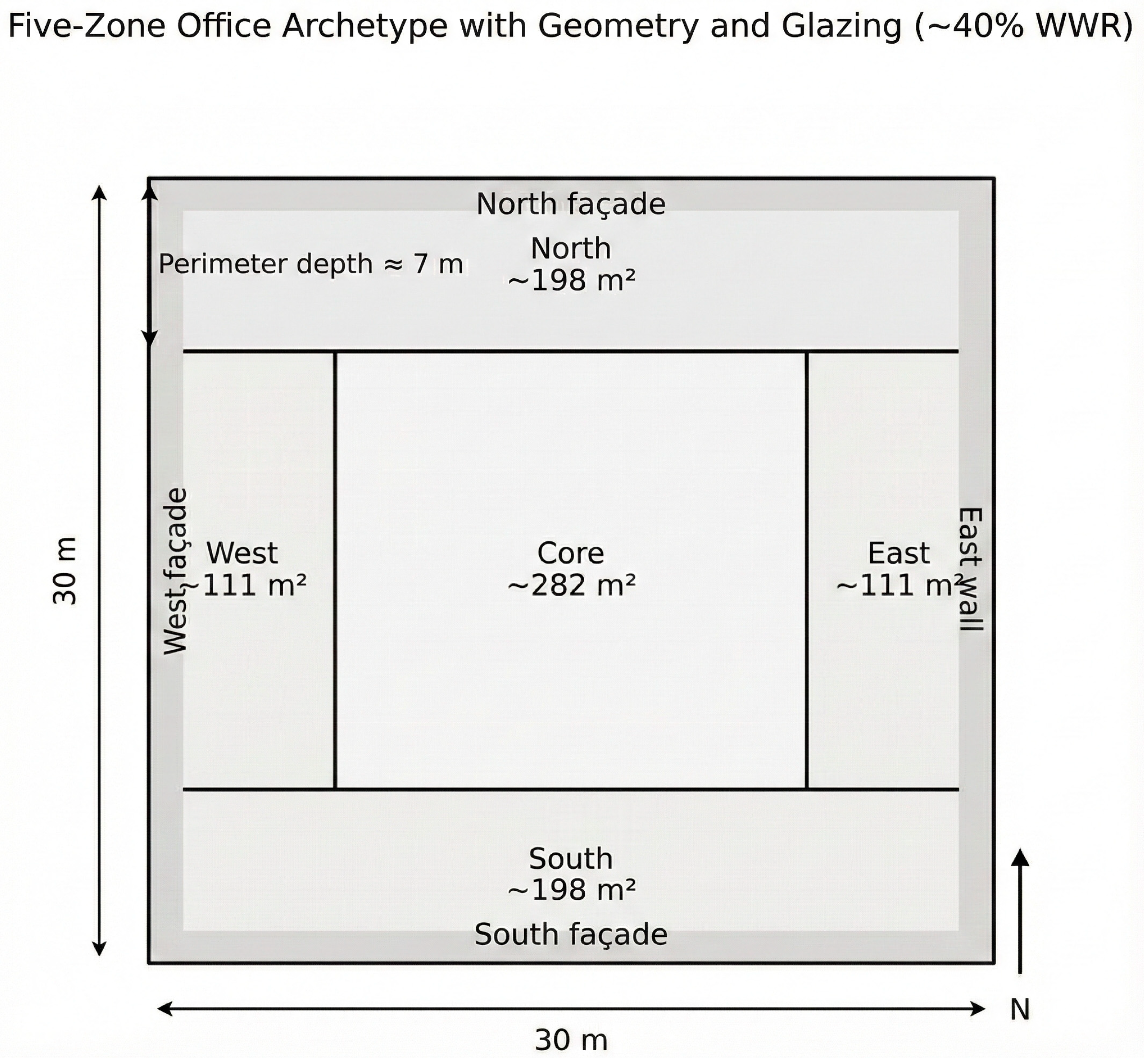
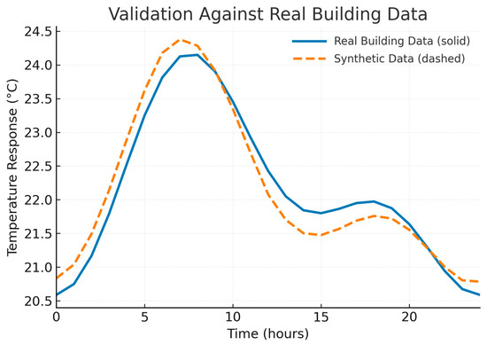
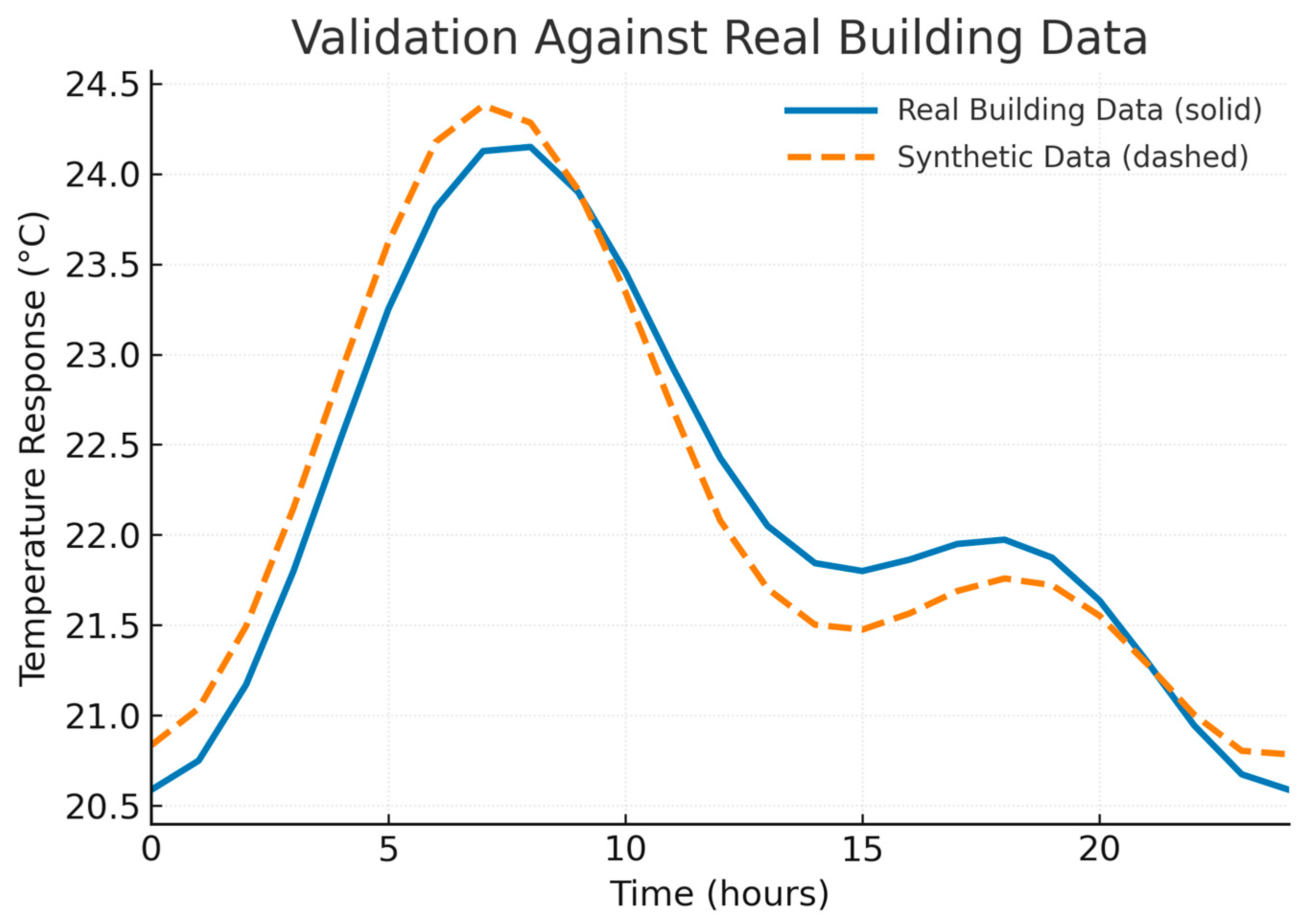
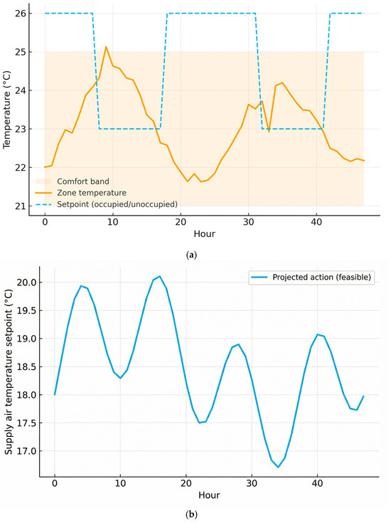
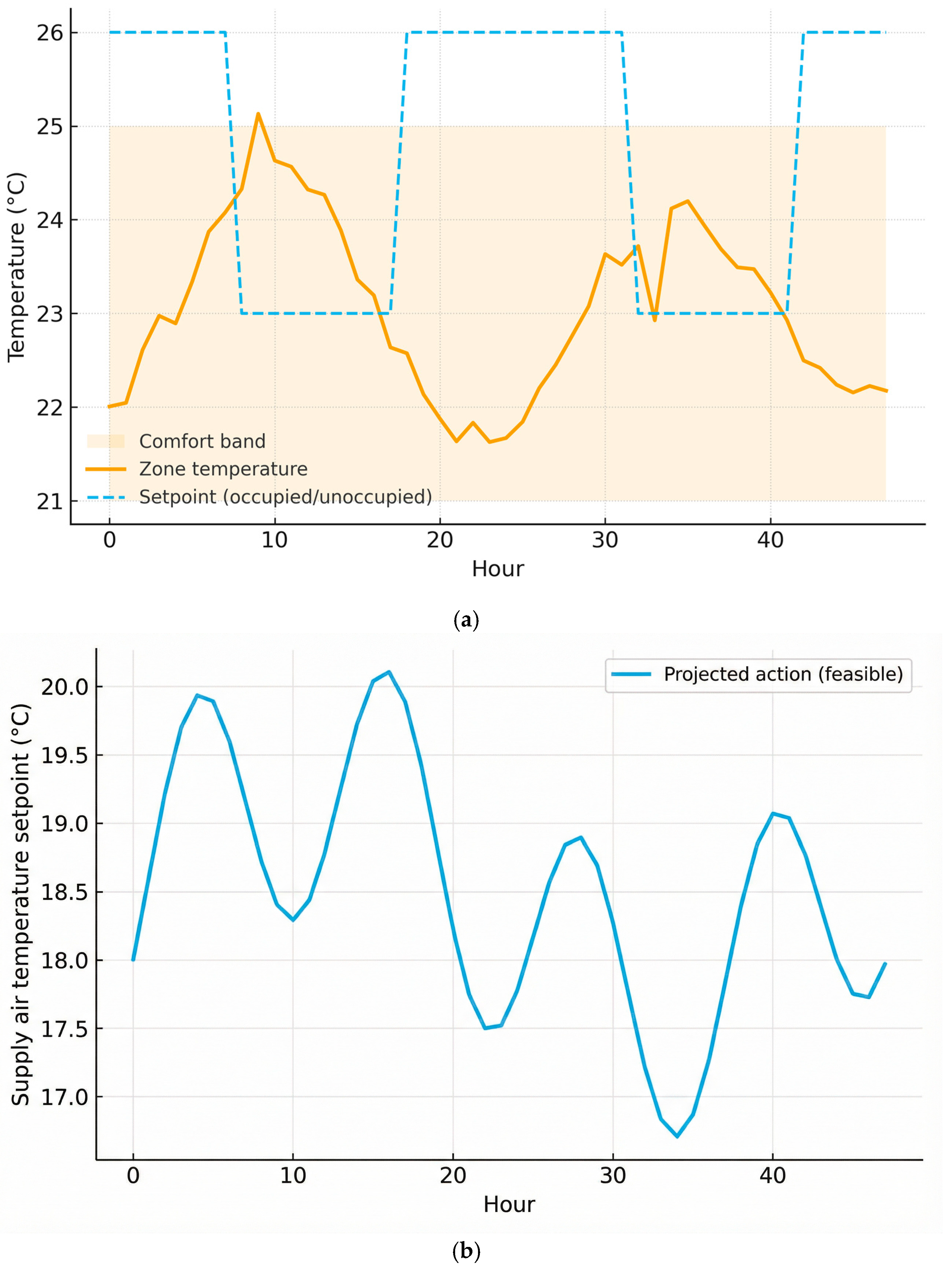
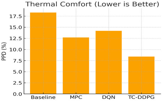
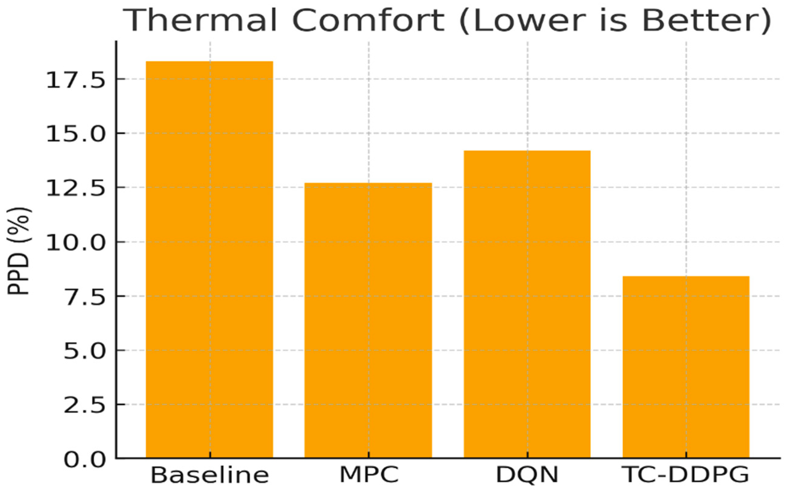
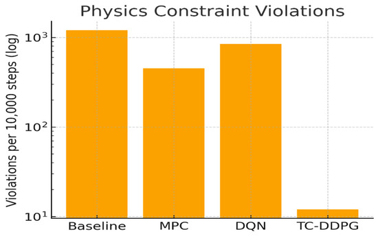
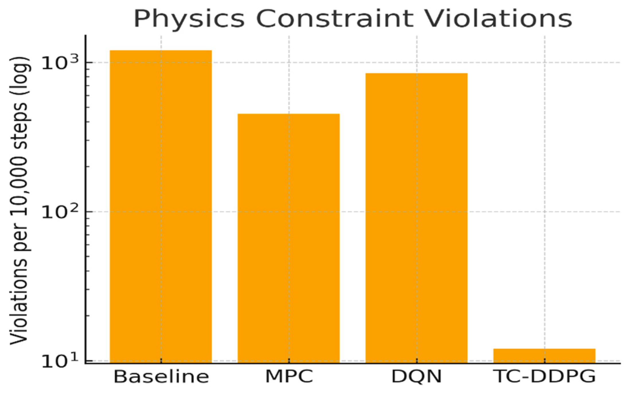
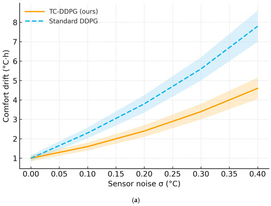
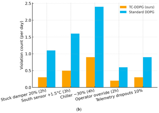
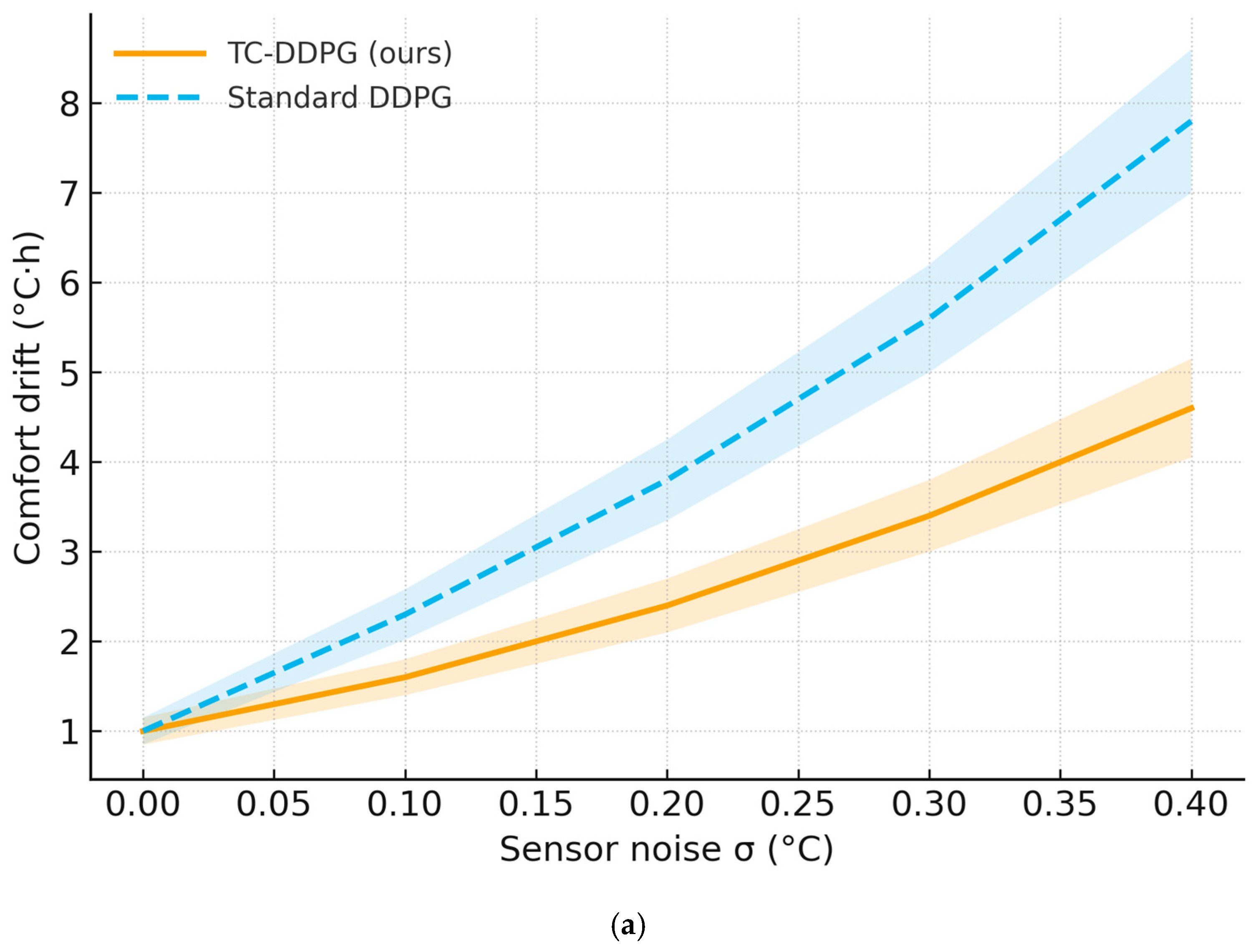
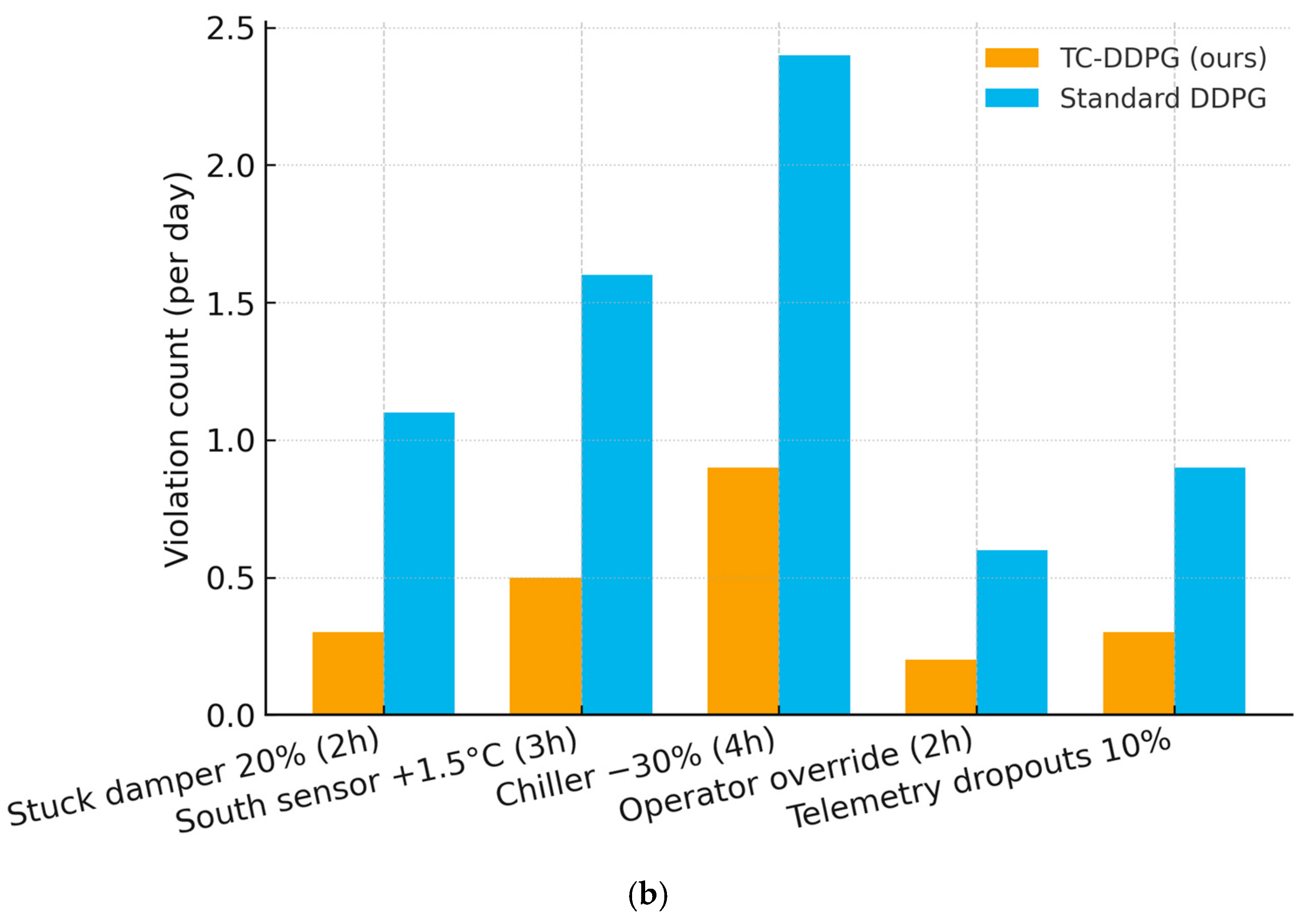
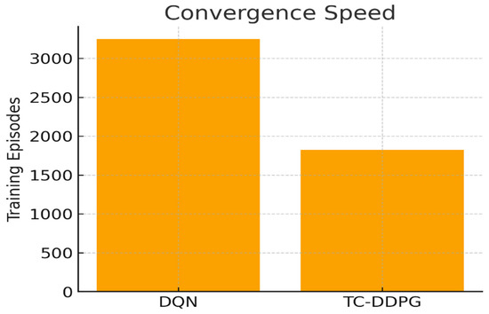
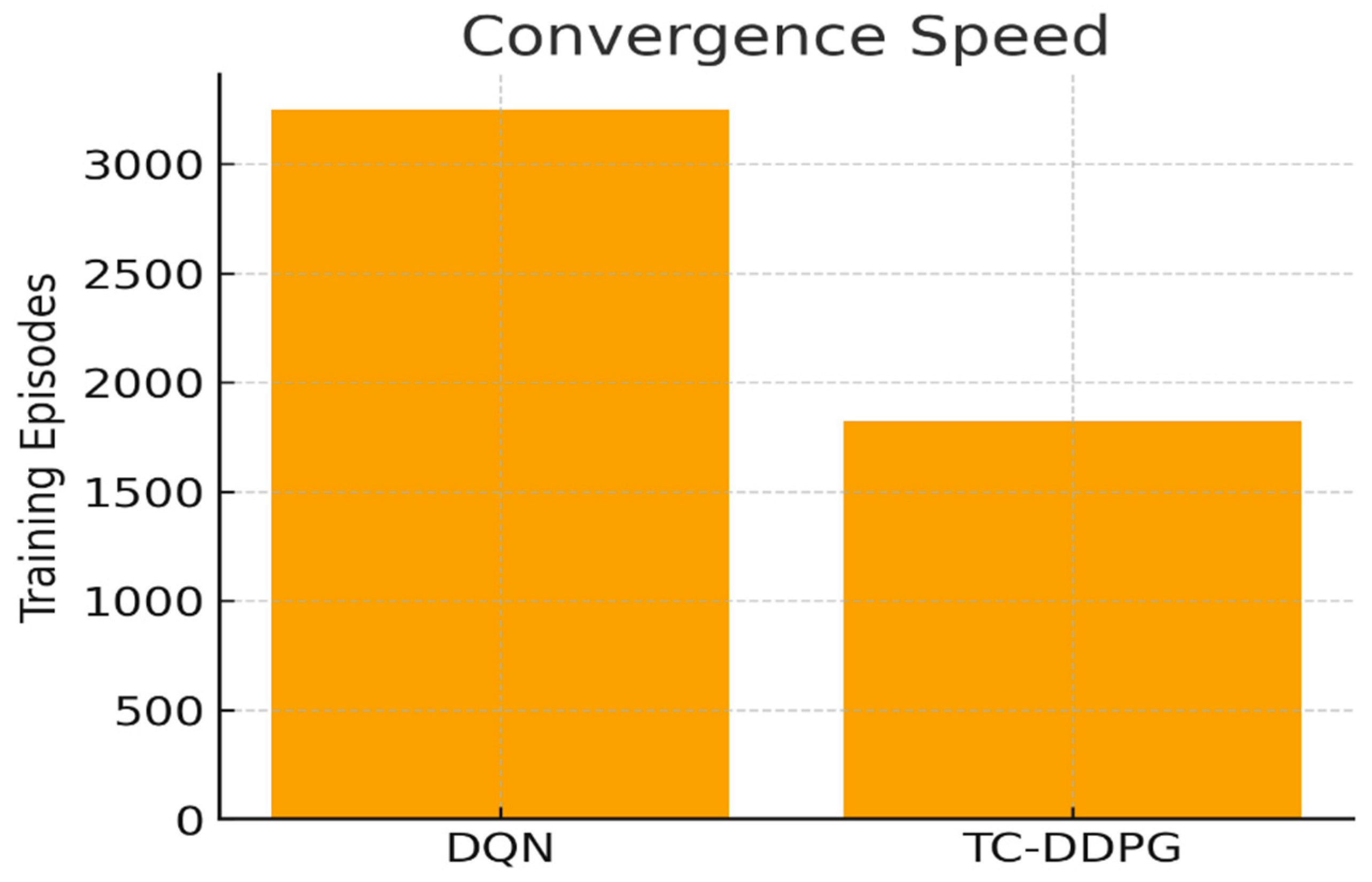
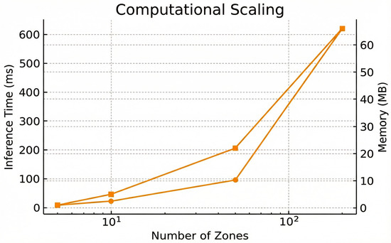
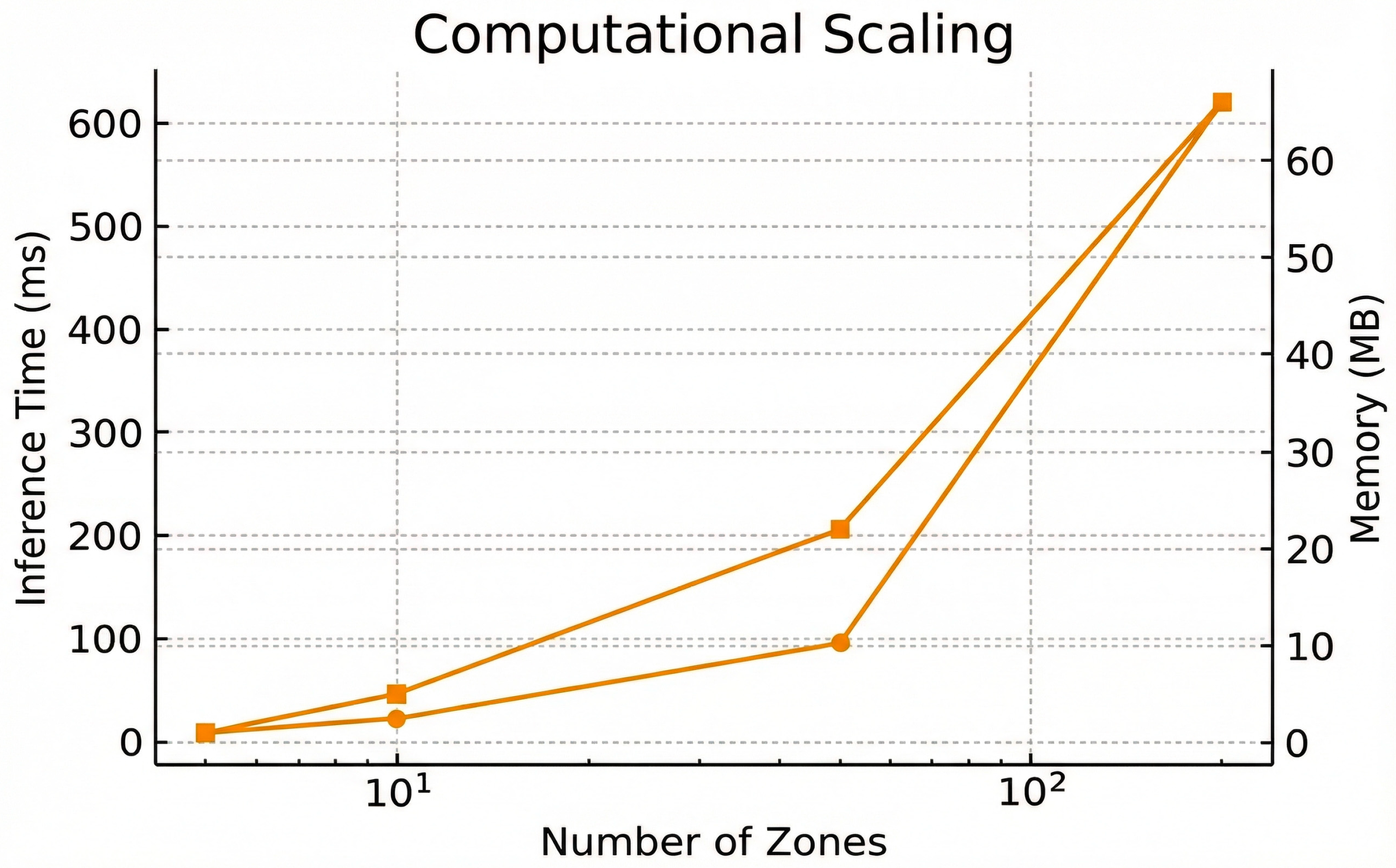
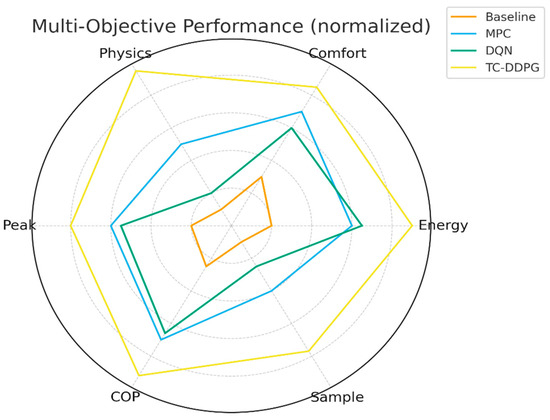
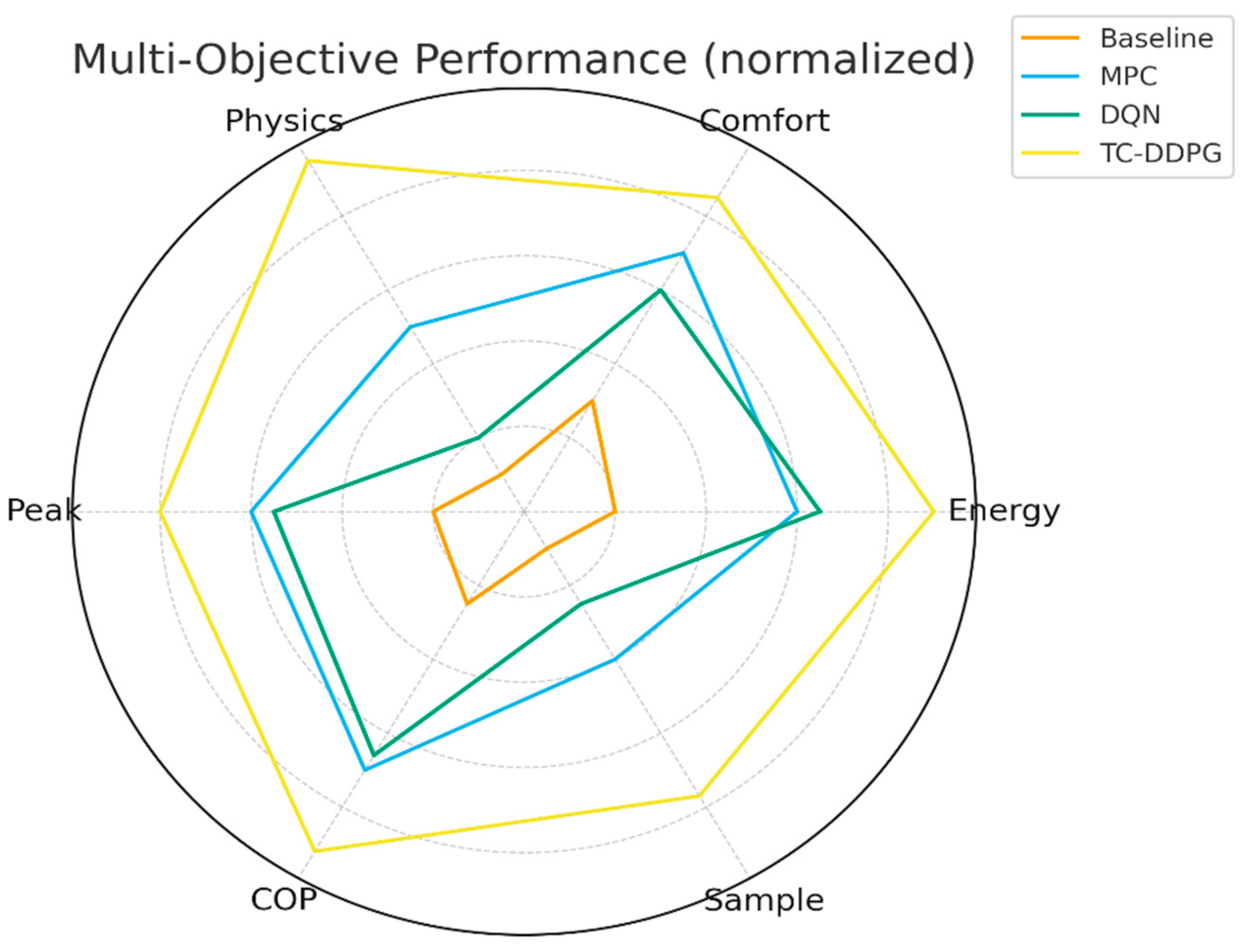
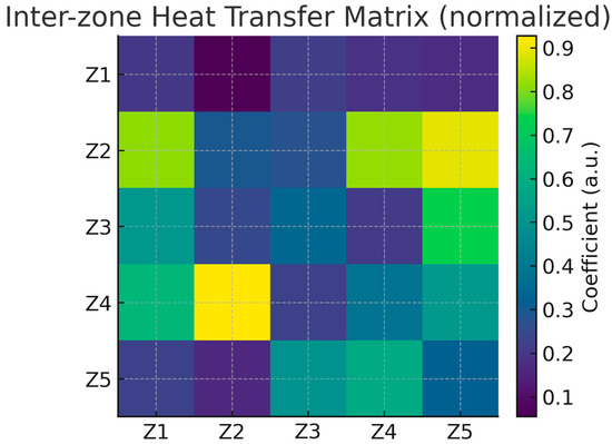
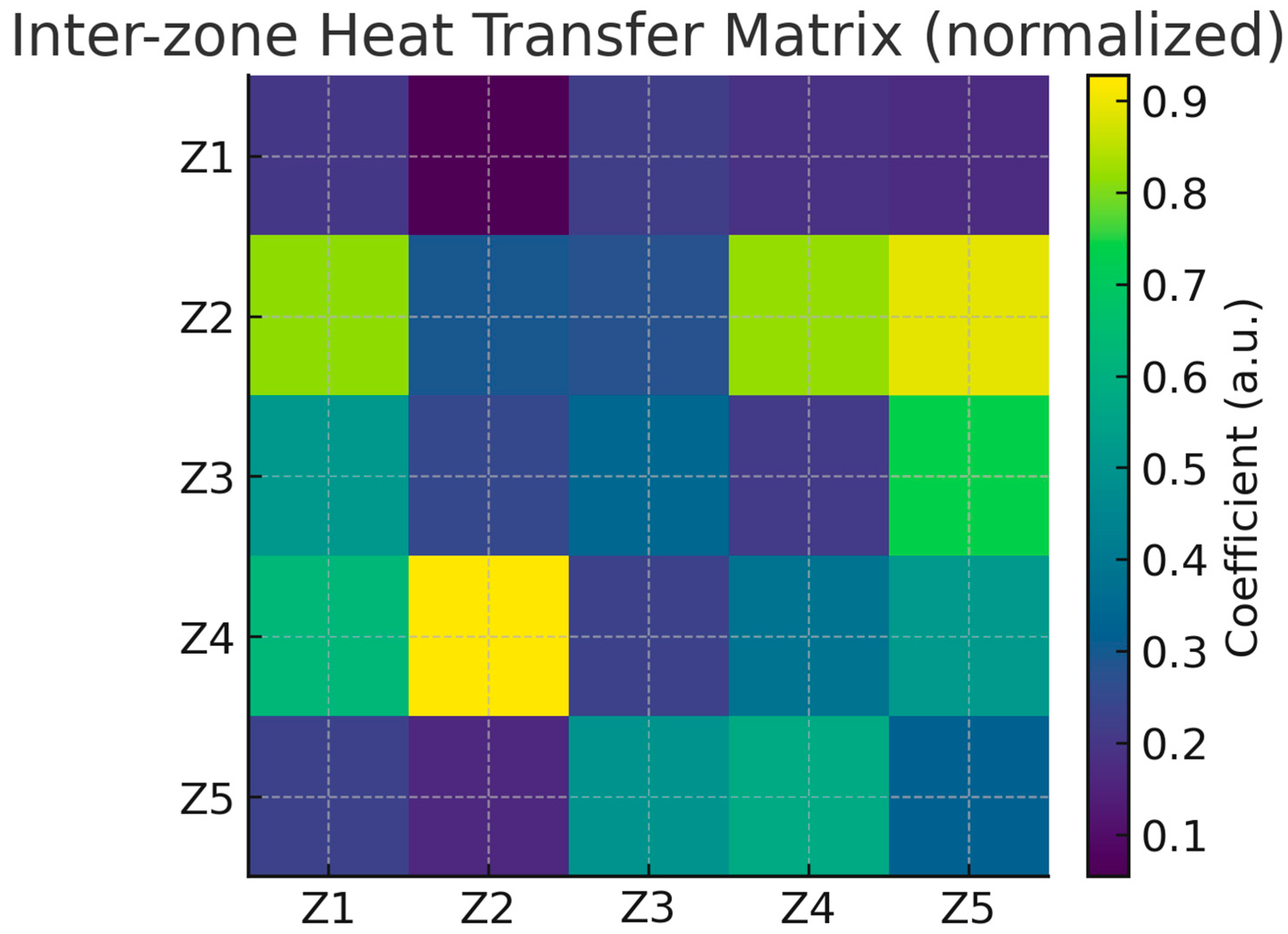
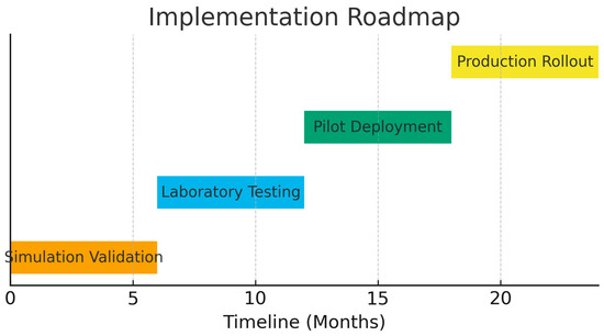
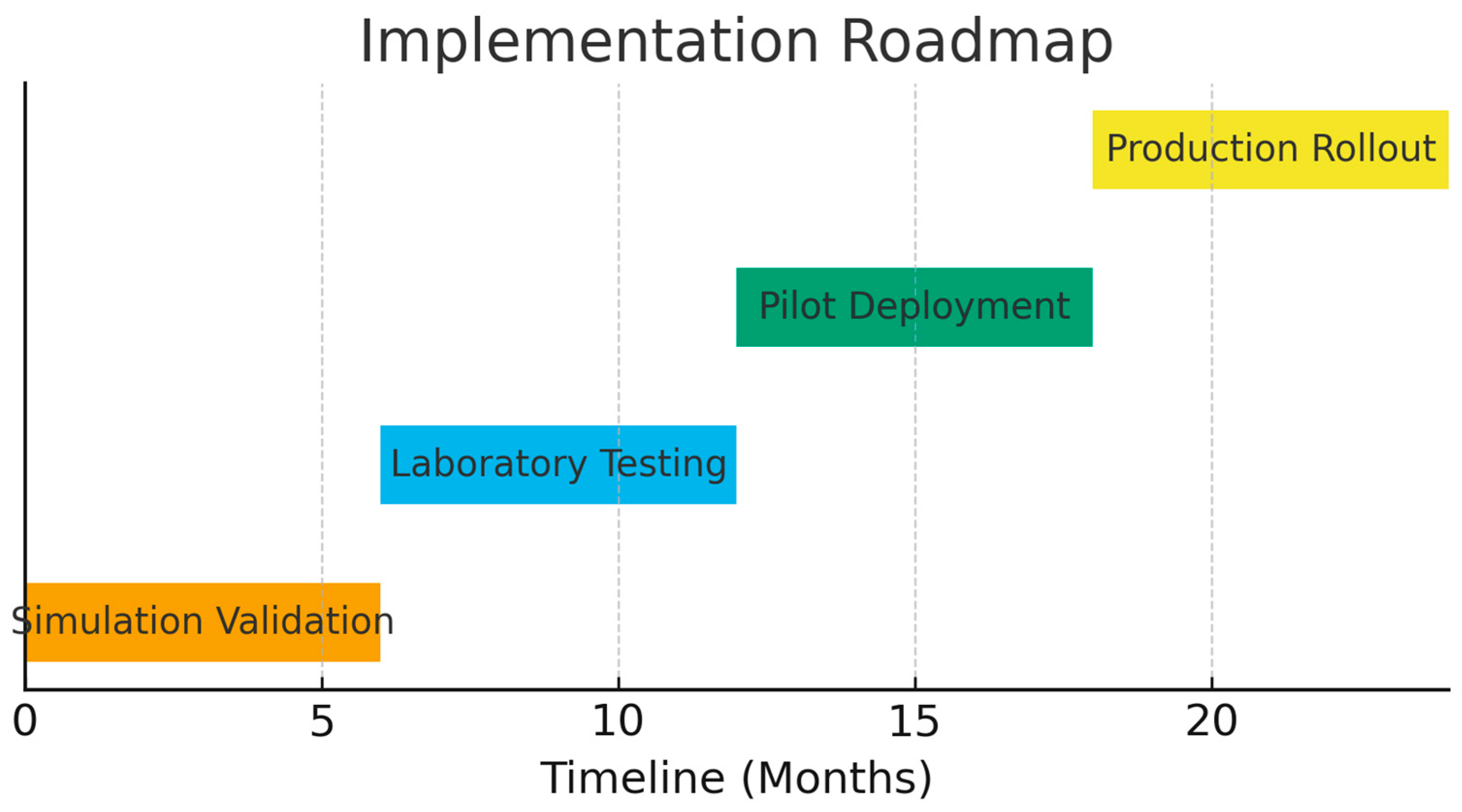
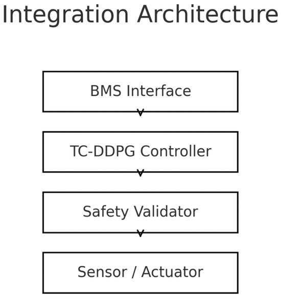
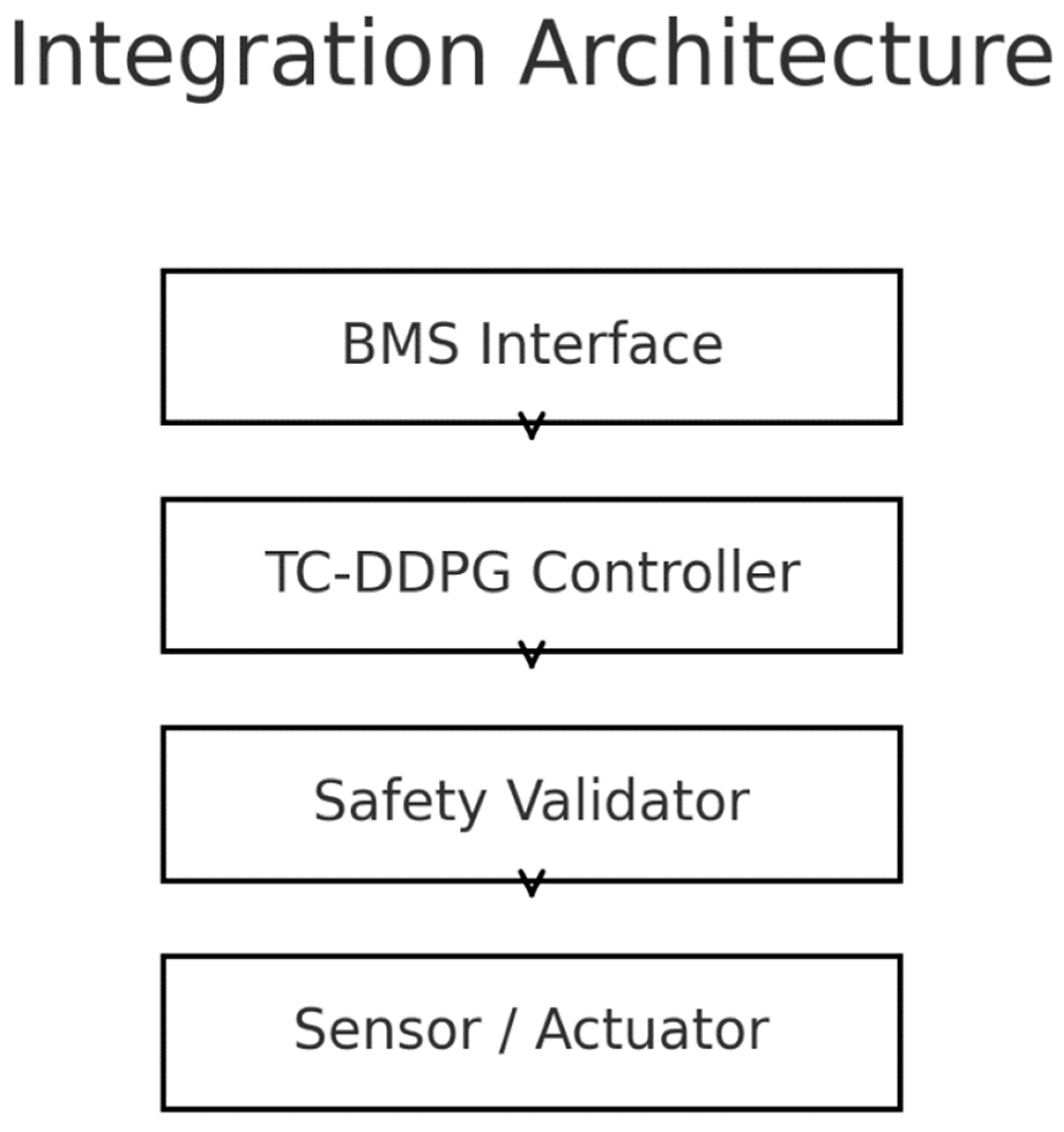

Disclaimer/Publisher’s Note: The statements, opinions and data contained in all publications are solely those of the individual author(s) and contributor(s) and not of MDPI and/or the editor(s). MDPI and/or the editor(s) disclaim responsibility for any injury to people or property resulting from any ideas, methods, instructions or products referred to in the content. |
© 2025 by the authors. Licensee MDPI, Basel, Switzerland. This article is an open access article distributed under the terms and conditions of the Creative Commons Attribution (CC BY) license (https://creativecommons.org/licenses/by/4.0/).