Article

Performance Prediction of a Vertical Downward Supply Direct Expansion Cooling System for Large Spaces Through Field Experiments

1
Department of Energy System Engineering, Graduate School, Seoul National University of Science and Technology, Seoul 01811, Republic of Korea
2
School of Architecture, Seoul National University of Science and Technology, Seoul 01811, Republic of Korea
*
Author to whom correspondence should be addressed.
Energies 2025, 18(23), 6160; https://doi.org/10.3390/en18236160
Submission received: 8 October 2025 / Revised: 8 November 2025 / Accepted: 19 November 2025 / Published: 24 November 2025
(This article belongs to the Section G: Energy and Buildings)

Abstract

Performance prediction of an air-cooled direct expansion (DX) vertical downward-supply cooling system applied to large spaces is a key element for achieving efficient control and energy savings. Recent studies have predominantly relied on complex artificial intelligence (AI)-based or high-dimensional models that require a large number of input variables to achieve high predictive accuracy. In contrast, limited research has focused on developing simple, interpretable, and practically applicable models based on field-measured data. To address this gap, the present study proposes a physically grounded multiple linear regression model with a minimal number of variables, which can be implemented in practice using only three standard sensors: indoor air temperature, outdoor air temperature, and airflow rate. Field data were refined through physical criteria derived from ASHRAE standards (steady-state operation and removal of outliers) and by identifying steady-state ranges using the Kernel Density Estimation (KDE) method. A total of 133,718 valid samples were used for analysis. The proposed model achieved a coefficient of determination (R2) of 0.93, a root mean square error (RMSE) of 2.86 kW, and mean absolute error (MAE) of 2.31 kW, corresponding to approximately ±6% deviation from measured cooling capacity. These results satisfy the typical accuracy criteria in the HVAC field (R2 > 0.9, error < 10%) and confirm high predictive reliability despite the model’s simplicity. The achieved accuracy implies that the proposed model can be extended to field-level performance prediction and energy-efficient operation. Comparison with second-order polynomial and nonlinear (1/Tout) models showed only marginal improvement in accuracy. Consequently, the proposed three-variable regression model introduces a practical framework for performance prediction and control of DX-type cooling systems that integrates simplicity, physical interpretability, and field applicability.

1. Introduction

1.1. Background

Conventional cooling systems for large-space buildings have traditionally relied on centralized air-conditioning systems, in which large-scale equipment regulates the thermal conditions of the entire space. However, facilities such as factories, gymnasiums, and atriums exhibit highly non-uniform thermal environments due to their high ceilings and uneven internal heat generation [1,2]. These characteristics often lead to vertical thermal stratification and localized thermal discomfort, posing significant challenges for efficient cooling design and control [3,4]. Moreover, recent studies have reported that non-uniform temperature distributions in such spaces can increase cooling energy consumption and reduce indoor thermal stability, underscoring the need for optimized thermal environment management and predictive control strategies [1,2,5].
To address these challenges, the HVAC industry has developed part-load-responsive control technologies that have evolved from conventional centralized systems. The Variable Air Volume (VAV) system improved energy efficiency by modulating airflow rates according to real-time cooling loads. More recently, Variable Refrigerant Flow (VRF) systems—based on direct expansion (DX) cooling—have been widely adopted in commercial buildings. By expanding the refrigerant directly within each indoor unit, VRF systems enable zone-level load responsiveness, providing operational flexibility and enhanced energy performance under part-load conditions. Comparative studies have demonstrated that VRF systems achieve greater energy savings than VAV systems [6] and that DX-based VRF configurations outperform conventional air-handling unit (AHU) systems in overall cooling energy efficiency [7].
The equipment investigated in this study follows the same technological lineage, adopting a DX-based vertical downward-supply modular cooling configuration. Each system consists of an indoor and an outdoor module, and multiple units can be installed in parallel to flexibly respond to varying cooling demands. If the cooling capacity of each unit can be reliably predicted, the system can dynamically adjust airflow rates and compressor capacities, thereby minimizing overcooling, avoiding excessive fan power consumption, and reducing overall energy use. This approach aligns with previous findings that system configuration directly influences energy performance and control responsiveness, reinforcing the advantages of distributed and modular system architectures [6,7].
Accordingly, this study defines the equipment as a Modular Direct Expansion (DX) Cooling System, comprising multiple vertical DX units that operate independently while collectively cooling a large indoor space. As a decentralized counterpart to conventional centralized systems, the modular DX configuration combines unit-level simplicity with scalable flexibility, making it particularly suitable for large industrial and semi-industrial applications. Its enhanced controllability and potential for energy savings contribute to both energy-efficient operation and improved thermal comfort in large-space environments.
In parallel, recent research has focused on data-driven characterization of cooling demand across large building portfolios [8] and on time-series load prediction for central air-conditioning systems in industrial facilities to support integrated production and facility management [9]. These developments underscore the growing need for predictive models that are not only accurate but also readily implementable within real-world control frameworks.
Therefore, this study proposes a minimal-variable regression model for predicting the cooling capacity of a modular DX system using a small number of sensors. The objective is to develop a model that ensures physical interpretability and practical applicability while maintaining computational simplicity. If adequate predictive accuracy and reproducibility are achieved, the model can be extended to support staging control, inter-unit airflow distribution, and optimal system operation, ultimately, contributing to energy-efficient, building-level control strategies.
Building upon this background, the following Section 1.2 reviews recent studies on prediction methodologies.

1.2. Literature Review

Recent research on building energy and cooling load prediction has explored a wide range of data-driven approaches. Deep learning-based methods have demonstrated very high accuracy in short-term cooling load forecasting [10], while hybrid models combined with time-series preprocessing have shown effectiveness in complex environments such as large airport terminals [11]. Neural network structures that combine multiple features have attempted to balance stability and accuracy [12], and prediction-control frameworks tailored for Dedicated Outdoor Air Systems (DOAS) have illustrated direct applicability to operation [13]. Studies predicting key state variables of DX units such as evaporating temperature with Long Short-Term Memory (LSTM) models have supported the feasibility of data-driven approaches for DX equipment [14], and in the cooling tower domain, Artificial Neural Network (ANN) models have shown advantages over conventional physical models such as the Poppe model [15]. Further extensions of ANN to include building envelope parameters and climate stress indices have emphasized the importance of modeling climate variability [16].
Beyond deep learning, various machine learning approaches have been proposed. In the residential building sector, ANN-based models have proven effective [17], while kernel-based models such as Gaussian Process Regression (GPR) have been applied to high-resolution load prediction [18]. Improved hybrid models, such as Particle Swarm Optimization–Least Squares Support Vector Machine (PSO-LSSVM), have further enhanced prediction accuracy [19]. Recent developments also include transfer learning, data integrity assessment, clustering-based feature extraction, and modified deep learning structures [8,9,20,21,22,23,24]. Hybrid models for VRF systems [25] and ANN-based performance prediction frameworks for DX and heat pump systems [26] have also been reported.
In addition, studies have increasingly sought to apply prediction results directly to control. For example, factory Heating, Ventilation, and Air Conditioning (HVAC) systems have demonstrated improved control performance through the application of Model Predictive Control (MPC), and follow-up studies by the same research group have confirmed similar results [27]. Large commercial buildings have adopted learning-based predictive control to balance energy savings and thermal comfort [28], and simplified adaptive models combined with genetic algorithms have been applied to supervisory and optimal control in central chiller plants [29]. These studies show that relatively simple and interpretable models, such as regression, adaptive models, and state-space models, can be effective for control applications, even without complex black-box neural networks.
While deep learning and hybrid models offer high predictive accuracy and scalability, their complexity, data requirements, and limited interpretability constrain their practical application to real-time control. In contrast, regression-based approaches allow physical interpretability of input-output relationships while maintaining structural simplicity and accuracy. Many regression-based studies have demonstrated the ability to empirically explain building-level energy performance [30], and feature engineering combined with regression has highlighted the importance of input variable design [31]. Regression-based predictions of office building performance have been systematically conducted since the early stages of energy modeling research [32], and nonlinear regression models have also been tested to link cooling load predictions to optimal operation strategies [33]. Furthermore, in hybrid hydronic systems, multivariate nonlinear regression has been used to stably predict operational performance, confirming the general applicability and validity of regression approaches [34].
Recent studies have also employed ensemble and regression-based learning to address the limitations of purely black-box approaches. For instance, a random-forest-based regression model has achieved high prediction accuracy even under nonlinear and noisy experimental conditions, demonstrating robust adaptability to fluctuating environments [35].
To systematically evaluate existing prediction models, this study conducted a quantitative comparison of representative works. Appendix A Table A1 summarizes references [10,11,12,13,14,15,16,17,18,19,20,21,22,23,24,25,26,27,28,29,30,31,32,33,34,35] in terms of model type, target system, number of input variables, and reported accuracy metrics (R2, RMSE, MAPE).
The comparison shows that machine- and deep-learning approaches, such as ANN, LSTM, CNN-Transformer, GPR, and LSSVM, generally achieved very high accuracy (typically R2 > 0.95 and MAPE < 3%) while using 3 to 14 input variables. These models effectively capture nonlinear relationships among multiple environmental parameters but tend to rely on extensive data preprocessing and complex training structures.
In contrast, regression-based approaches show a broader range of model complexity, employing roughly 4 to 27 variables. Their predictive accuracy often improves with the inclusion of nonlinear terms, and several multivariate models reported R2 values around 0.96. Notably, some studies demonstrated competitive performance with only a few input variables. For example, a four-variable linear regression achieved MARE < 8% [24], and a four-variable nonlinear regression reached R2 = 0.963 [34]. These results indicate that compact, physically meaningful formulations can still yield high accuracy.
Within the machine-learning category, Mohanraj et al. [26] applied an ANN with only two input parameters (solar intensity and ambient temperature) to predict the performance of a solar-assisted heat-pump system, obtaining R2 ≈ 0.999 for multiple outputs. This illustrates that a small number of inputs is not exclusive to regression methods. In addition, Hu et al. [35] demonstrated that a random-forest model maintained strong robustness (R2 = 0.916) under environmental noise, highlighting its partial interpretability through feature-importance analysis.
Overall, the evidence from Table A1 indicates that recent prediction studies have primarily focused on improving accuracy by increasing model complexity, either through the use of deep or hybrid machine-learning frameworks or by expanding the number of input variables and nonlinear terms within regression models.
Hybridized approaches combining AI and statistical techniques have become increasingly common, while regression-based methods have also incorporated feature engineering or optimization algorithms to enhance performance.
However, few studies have explored whether a simple, physically interpretable regression formulation with a minimal number of measurable variables could achieve comparable predictive accuracy.
This observation highlights the need for a more accessible and transparent modeling strategy that can balance accuracy, interpretability, and practical applicability in real-world HVAC systems.
These insights form the basis for identifying the research gap and defining the objectives presented in Section 1.3.

1.3. Research Gap and Objectives

Despite the remarkable progress of data-driven prediction in HVAC systems, most recent studies have relied on increasingly complex structures such as deep neural networks, hybrid learning frameworks, or regression models with many variables to pursue marginal gains in predictive accuracy.
As a result, interpretability and practical applicability have often been compromised.
To date, little attention has been given to determining whether a simple regression-based approach, built upon a few physically meaningful variables, can deliver comparable performance while retaining transparency and ease of implementation for control purposes.
This study addresses this gap by developing and validating a physically interpretable, minimal-variable regression model for a large-space DX cooling system using field-measured data.
In contrast, regression-based approaches offer transparent and computationally efficient formulations. Yet, many of these models were developed under simplified or laboratory-scale conditions and have not been validated for large-space DX systems, which exhibit strong spatial temperature gradients and variable airflow patterns.
Moreover, few previous studies have critically integrated the strengths and limitations of both approaches. Most prior works have focused either on improving prediction accuracy or on simplifying model structure, while the balance between accuracy, interpretability, and control applicability has rarely been addressed.
In particular, there is a lack of regression models that can directly express the physical sensitivity of cooling performance to key measurable variables (e.g., indoor temperature, outdoor temperature, and airflow rate), and that can be readily implemented into control frameworks for large-scale field operation.
Therefore, the objective of this study is to develop and validate a physically interpretable regression model for a large-space direct expansion (DX) cooling system, derived from field-measured data. The proposed model aims to achieve high predictive accuracy with a minimal number of input variables, while preserving physical interpretability and direct control applicability. Ultimately, this study seeks to bridge the gap between data-driven prediction and practical control-oriented modeling, providing a foundation for optimal and energy-efficient operation of large-space DX cooling systems.
In summary, this study introduces an innovative regression-based prediction framework that bridges the gap between black-box deep-learning models and traditional physically interpretable regression approaches. The proposed framework aims to achieve high predictive accuracy with a minimal set of input variables, while maintaining transparency and direct applicability to control strategies for large-space DX systems.
The remainder of this paper is organized as follows.
Section 2 presents the experimental setup, data preprocessing, regression methodology, and validation procedures. Section 3 discusses the regression results, focusing on predictive accuracy and the sensitivity of key parameters. Section 4 interprets the physical implications and control applicability of the proposed model. Finally, Section 5 concludes the paper with the main findings and future research directions.
Overall, this integrated framework emphasizes both the methodological innovation and the systematic organization of the study.

2. Materials and Methods

2.1. Overview

The methodology of this study was designed to bridge the conceptual framework and the practical technical route in a coherent and traceable manner. This research stemmed from the recognition that most data-driven prediction models for HVAC systems—particularly AI-based approaches—tend to prioritize accuracy at the expense of interpretability. To address this limitation, the study was initiated with the hypothesis that the cooling capacity ( Q ˙ c) of a modular DX heat pump system can be accurately predicted using a minimal set of physically meaningful variables. Specifically, indoor air temperature (Tin), outdoor air temperature (Tout), and airflow rate ( V ˙ ) were identified as the core variables that collectively represent the thermal load, environmental stress, and controllable operational state of the system. This conceptual foundation emphasized simplicity, physical interpretability, and direct applicability to control.
Building on this conceptual premise, the research was technically implemented through a systematic sequence of field measurement, data refinement, regression modeling, and validation. Field experiments were conducted on a modular DX heat pump installed in a factory testbed, and cooling capacity was calculated using the air-side enthalpy method under diverse operating conditions. Multi-stage data filtering was applied to remove unstable or physically implausible states, followed by regression modeling using combinations of the identified core variables. The resulting models were evaluated through multiple statistical indicators (R2, Adj R2, RMSE, MAE) and physical consistency checks. Finally, the applicability of the proposed model was assessed for potential integration into airflow-based control strategies and modular operation.
Figure 1 illustrates this integrated research roadmap, demonstrating how the conceptual logic of the study (thought path) was translated into a technical implementation route from hypothesis formation to field execution, modeling, and validation.
Stage 1 defines the conceptual framework based on physical reasoning, Stage 2 implements field measurement and regression analysis, and Stage 3 validates the model for control-oriented applications.

2.2. Experimental Setup and Data Measurement

This section introduces the target equipment and the test site, and presents the operating conditions under which the experiments were conducted. It then describes the measured variables, the specifications and installation of the measuring instruments, and the procedures for acquiring key parameters such as temperature, humidity, pressure, refrigerant mass flow rate, and power consumption that are necessary for calculating cooling capacity. Finally, the data logging interval and synchronization procedures are briefly mentioned to provide an overview of the dataset used for subsequent analysis.

2.2.1. Experimental Equipment and Test Site

While ASHRAE Standard 37 specifies laboratory-rated conditions [36], this study was conducted under actual field operating environments to reflect diverse load fluctuations. Therefore, instead of being limited to a single standardized condition, data were collected under varying indoor and outdoor temperatures and airflow rates, representing the variability of real large-space cooling systems. This approach enhances the practical applicability of the proposed model. The fundamental principles of measurement and calculation, including the enthalpy-difference method and stability considerations for data reliability, followed the guidelines of ASHRAE 37.
The experiment was conducted in a real lightweight sandwich-panel factory building equipped with a single modular vertical downward-supply DX cooling unit. The detailed specifications of the test site, equipment, and operating conditions are summarized in Table 1.
Although this study investigated only one DX cooling unit in a single factory-type building, this configuration was intentionally selected to establish a clear, unit-level performance model under controlled yet realistic field conditions. By isolating a single unit, the analysis enabled precise quantification of the fundamental relationships among indoor air temperature, outdoor air temperature, and supply airflow rate, free from the confounding effects of inter-unit load sharing or complex control interactions. The chosen test site—a lightweight sandwich-panel factory with low thermal mass and high load variability—represents a typical industrial or warehouse building in Korea, where modular DX systems are widely employed. Consequently, the findings can be regarded as representative of general large-space environments. Future work will extend this approach to multi-unit and multi-zone configurations to verify scalability and system-level applicability.

2.2.2. Measuring Instrument and Uncertainty Estimation

In this study, calibrated sensors were installed to measure both air-side and refrigerant-side state variables as well as the system power consumption. Indoor and outdoor air temperatures and relative humidity were monitored using temperature–humidity sensors, while additional T-type thermocouples were used to record air and refrigerant temperatures at key locations. The refrigerant-side pressures and mass flow rate were measured using pressure transducers and a Coriolis-type mass flow meter, respectively, and the total power input was recorded through a digital sampling power meter.
Detailed specifications and measurement ranges for all instruments are summarized in Table A2 of the Appendix A.
The measurement uncertainties were evaluated based on the instrument specifications summarized in Appendix A Table A2, and the overall uncertainty of the cooling-capacity calculation was derived using the standard propagation-of-error approach. The uncertainty of the calculated cooling capacity ( u Q ˙ c ) was determined from the combined effects of the airflow measurement and the temperature-difference measurement according to the following representative Equation (1).
u Q ˙ c Q ˙ c = u V ˙ a i r V ˙ a i r 2 + u T T 2
In this expression, u V ˙ a i r is the standard uncertainty of the measured air volume flow rate and u T is the standard uncertainty of the measured air temperature difference between the inlet and outlet of the indoor unit. The air volume flow rate was determined using a Pitot-tube method with a differential-pressure transducer following ASHRAE 111 [37] and ISO 3966 [38]. A five-point traverse was performed for each fan-speed step. The combined relative uncertainty of the airflow measurement, which accounts for the transducer accuracy, Pitot-coefficient calibration, partial traverse sampling, and duct-area measurement, was estimated to be approximately ±3 to ±4% under field conditions.
The temperature difference uncertainty was obtained from two independent temperature sensors (±0.5 °C each), resulting in a combined uncertainty of u T = 0.707 °C. Considering the measured range of ΔT in the dataset (from the smallest 9.3 °C to the largest 22.7 °C), the propagated relative uncertainty of the cooling capacity was calculated to vary from approximately ±8 percent at ΔT = 9.3 °C to about ±5 percent at ΔT = 22.7 °C. Because the regression model was developed using steady-state averaged data, which represent 30 min mean values under stable compressor and fan operation, the statistical uncertainty of the averaged measurements further decreases with the number of samples. As a result, the effective overall uncertainty converges to approximately ±3 to ±5 percent. This range satisfies the ASHRAE 37 recommendation that total calorimetric measurement uncertainty remain within ±5 percent. The refrigerant mass-flow meter (RHM 08 GNT, Rheonik Messgeräte GmbH, Odelzhausen, Germany) was recorded only for diagnostic and filtering purposes (for instance, to identify EEV-closure conditions) and was not used in the air-side capacity calculation.
For example, assuming airflow uncertainty of ±1% and temperature sensor accuracy of ±0.707 °C, the propagated uncertainty can be calculated as follows:
u Q ˙ c Q ˙ c = 0.01 2 + 0.707 9.3 2 = 0.0001 + 0.00578 = 0.0767 ( 7.7 % )

2.2.3. Installation of Measuring Instruments

The measuring instruments were installed to monitor both air-side and refrigerant-side parameters for comprehensive performance evaluation under various operating conditions.
Temperature and humidity sensors (Testo 6621, Testo SE & Co. KGaA, LenzKirch, Germany) were installed at the inlet and outlet of the indoor unit to measure the supply air conditions and the air state after passing through the evaporator. Dry-bulb temperature sensors were placed at the condenser inlet and outlet of the outdoor unit to monitor the condenser-side conditions, while temperature (T-type Sensor, Dongyang Tech, Bucheon, Republic of Korea) and pressure (Setra Systems, Inc., Boxoborough, MA, USA) sensors were installed at the refrigerant inlet and outlet to enable enthalpy-based performance calculations.
All sensors were connected to a data logger (GL-820, Graphtec Corporation, Yokohama, Japan) and recorded at 1 s intervals. Power consumption data were measured separately using a power meter (CW-240, Yokogawa Electric Corporation, Tokyo, Japan) and synchronized based on time stamps. This configuration was designed to correspond directly to the variables required for calculating sensible, latent, and total cooling capacity.
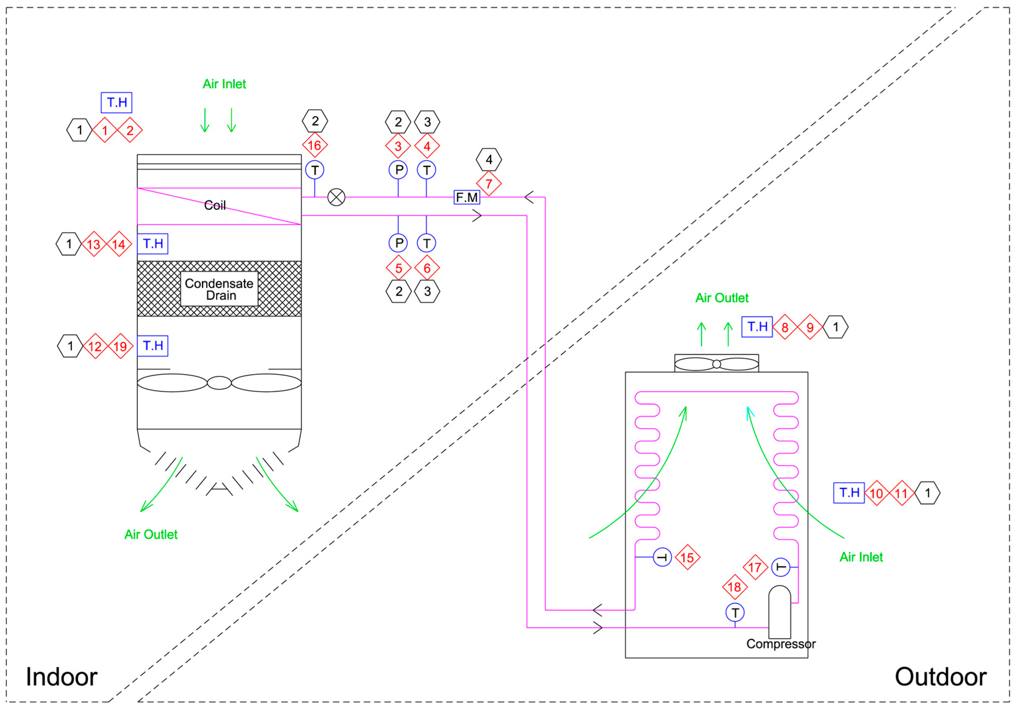
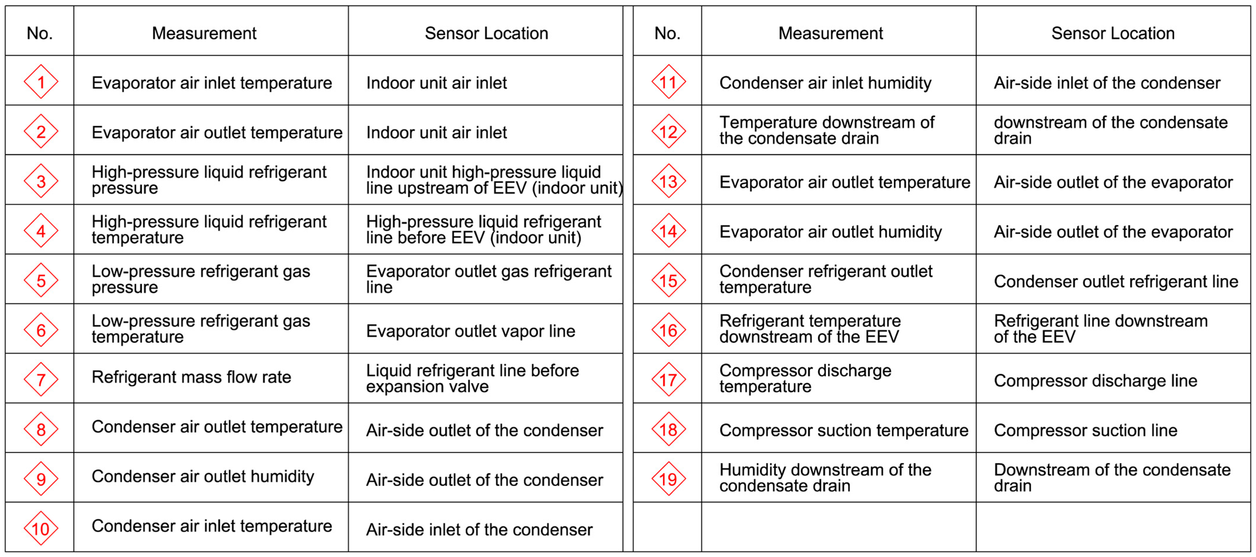
Detailed schematics, sensor layouts, and installation photographs are provided in Appendix A Figure A1, Figure A2, Figure A3 and Figure A4, which include the system diagram and sensor locations (Figure A1), detailed measurement layouts (Figure A2), the symbol index used in the analysis (Figure A3), and photographs of the experimental setup (Figure A4).
The airflow rate was determined using the Pitot tube differential pressure method, following the velocity–area method procedures specified in ASHRAE Standard 111 [37] and ISO 3966 [38]. Instead of conducting a full cross-sectional traverse, airflow measurements were taken at five representative points across the duct cross-section for each fan speed step (20, 40, 50, 60, 80, 100%). The average velocity was calculated using Equation (2), and the airflow rate was obtained by multiplying the cross-sectional area by the average velocity as shown in Equation (3).
v = 2 P ρ
V ˙ = A v
The representative airflow rate obtained for each fan speed step was applied to all datasets collected under the same fan speed condition. Although this procedure simplified the full traverse, it maintained the concept of multi-point averaging and complied with standard field measurement methodologies. In this study, fan speed (%) and airflow rate (m3/s) were used together depending on the context. Since the equipment was operated with stepwise fan speed control (20, 40, 50, 60, 80, 100%), representative airflow values were pre-measured for each step and used as reference values. While the control method may differ for other equipment, in this study the values listed in Table 2 were consistently applied to all data under the same operating conditions.

2.2.4. Data Measurement and Acquisition

The measurements were conducted on non-operating days of the factory, so internal heat gains from occupants and equipment could be neglected. The cooling load was therefore primarily determined by external conditions such as solar radiation and heat transfer through the building envelope [32]. As a limitation, envelope U-values and infiltration air rates were not quantified. In some tests, the entrance doors were intentionally opened under high outdoor temperature conditions to secure diverse operating scenarios. The measurements were performed during the cooling season in Korea (June to September), and the dataset included a wide range of operating conditions, from approximately 40% partial load up to above rated load.
Although the building height was 7.35 m and vertical stratification could potentially occur, multi-point temperature sensors were not installed. Instead, the indoor unit inlet temperature was used as the representative indoor air temperature. This approach has also been employed in previous large space studies [39,40], which showed that single-point measurements can be representative. Nevertheless, the uncertainty associated with stratification in large spaces has been reported [41], and was considered a limitation in this study.
Data were collected through the measuring instruments described earlier, with all sensor signals recorded at 1 s intervals using a GL-820 data logger. Power consumption was measured separately with a digital power meter and synchronized based on time stamps. This configuration ensured a stable dataset for calculating sensible, latent, and total cooling capacities, as well as for securing reliable input variables for regression analysis.
Unlike laboratory-based rated condition tests in the ASHRAE Standard 37 [36], this study was carried out under diverse outdoor conditions reflecting actual field operation. As a result, load fluctuations and system responses that are difficult to capture in laboratory environments were included in the dataset. At the same time, reproducibility was ensured through clearly defined measurement and data processing procedures.

2.3. Data Processing and Filtering

2.3.1. Cooling Capacity Calculation

The cooling capacity in this study was calculated using the enthalpy-difference method specified in ASHRAE Standard 37 [36]. This method separates cooling capacity into sensible and latent components, which are calculated individually and then summed to obtain the total cooling capacity.
First, the air mass flow rate was calculated from the volumetric airflow rate derived earlier in Equation (2), multiplied by the air density, as expressed in Equation (4).
m ˙ a i r = ρ V ˙
The sensible cooling capacity ( Q ˙ s e n s ) was calculated using the air mass flow rate, the specific heat of air at constant pressure, and the dry-bulb temperature difference between the indoor unit inlet and outlet, as shown in Equation (5).
Q ˙ s e n s = m ˙ a i r c p ( T i n T o u t )
The latent cooling capacity ( Q ˙ l a t ) was obtained by multiplying the air mass flow rate by the change in latent heat of vaporization associated with the difference in humidity ratio, as defined in Equation (6).
Q ˙ l a t = m ˙ a i r h f g ( w i n w o u t )
Here, the humidity ratio ( w ) was calculated from the measured dry-bulb temperature and relative humidity, together with standard atmospheric pressure, by applying psychrometric relations provided in the ASHRAE Handbook Fundamentals (2009) [42]. The actual implementation used the built-in functions of Engineering Equation Solver (EES, F-Chart Software, Madison, WI, USA).
In these equations, m ˙ a i r is the supply air mass flow rate, c p is the constant pressure specific heat of air, h f g is the latent heat of vaporization of water vapor, and w is the humidity ratio. The total cooling capacity ( Q ˙ t o t ) was obtained as the sum of sensible and latent capacities, as expressed in Equation (7).
Q ˙ t o t = Q ˙ s e n s + Q ˙ l a t
This enthalpy-based method reflects both sensible heat removal by temperature reduction and latent heat removal by moisture extraction. It is widely used in cooling performance evaluation and is consistent with the guidelines of the ASHRAE Standard 37 [36].
Finally, the calculated cooling capacity data were integrated with the collected time-series measurements to construct a unified dataset. The total number of data samples obtained was 133,718.

2.3.2. Data Filtering

A multi-stage data filtering procedure was performed to ensure the physical validity and reliability of the experimental dataset. Since the raw data were collected at 1 s intervals, transient disturbances such as compressor start-up and shutdown, fan operation fluctuations, and door openings in the test space could significantly affect the measured cooling capacity. Therefore, before developing regression-based performance prediction models, it was essential to select only the data representing steady-state operating conditions. Table 3 summarizes the filtering criteria and their rationales.
1.
Step 1. Compressor outlet temperature threshold (≥70 °C)
ASHRAE Standard 37 [36] requires a minimum of 30 min of steady-state operation during performance evaluation. In this study, compressor discharge temperature was used as an indicator of stability. Measurements showed that after approximately 30 min of operation, the discharge temperature stabilized above 70 °C, fluctuating within a limited range depending on load conditions. In contrast, during start-up the discharge temperature remained below 70 °C due to unstable compression and superheating. Therefore, only data with compressor discharge temperatures above 70 °C were retained, ensuring consistency with ASHRAE guidelines.
2.
Step 2. Refrigerant flow validation (expansion valve closure removal)
ASHRAE Standard 41.9 [43] emphasizes that valid flow conditions must be maintained when measuring refrigerant mass flow. In this study, it was observed that when the electronic expansion valve (EEV) was fully closed, refrigerant mass flow dropped to zero. These cases corresponded to compressor off-cycles or protective control operations, which are not representative of normal cooling operation. Such data were therefore removed.
3.
Step 3. Outdoor air inlet temperature threshold (≤40 °C)
AHRI Standard 210/240 [44] specifies 35 °C (95 °F) outdoor dry-bulb temperature as a standard test condition. However, since this study was based on field measurements, a wider range of outdoor conditions was included. According to local meteorological data, maximum summer temperatures in Seoul during the past five years did not exceed 37 °C, although rare extreme cases such as the 41 °C record in Hongcheon in 2018 have been reported. Accordingly, an upper threshold of 40 °C was adopted. Data exceeding this threshold were regarded as outliers or sensor errors and were removed. This criterion maintained consistency with rating standards while reflecting realistic climate conditions.
4.
Step 4. Outdoor unit ΔT stability (≥5.5 °C)
ASHRAE Standard 41.2 [45] requires stable and uniform airflow across heat exchangers to ensure reliable performance testing. Analysis of the experimental data indicated that when the outdoor fan was off or in early operation stages, the condenser inlet–outlet temperature difference (ΔT) was below 5.5 °C. Under such conditions, heat rejection was insufficient, and steady-state operation could not be assumed. Therefore, data with ΔT less than 5.5 °C were excluded as non-representative.
5.
Step 5. Indoor unit ΔT stability (±2 °C from KDE mode)
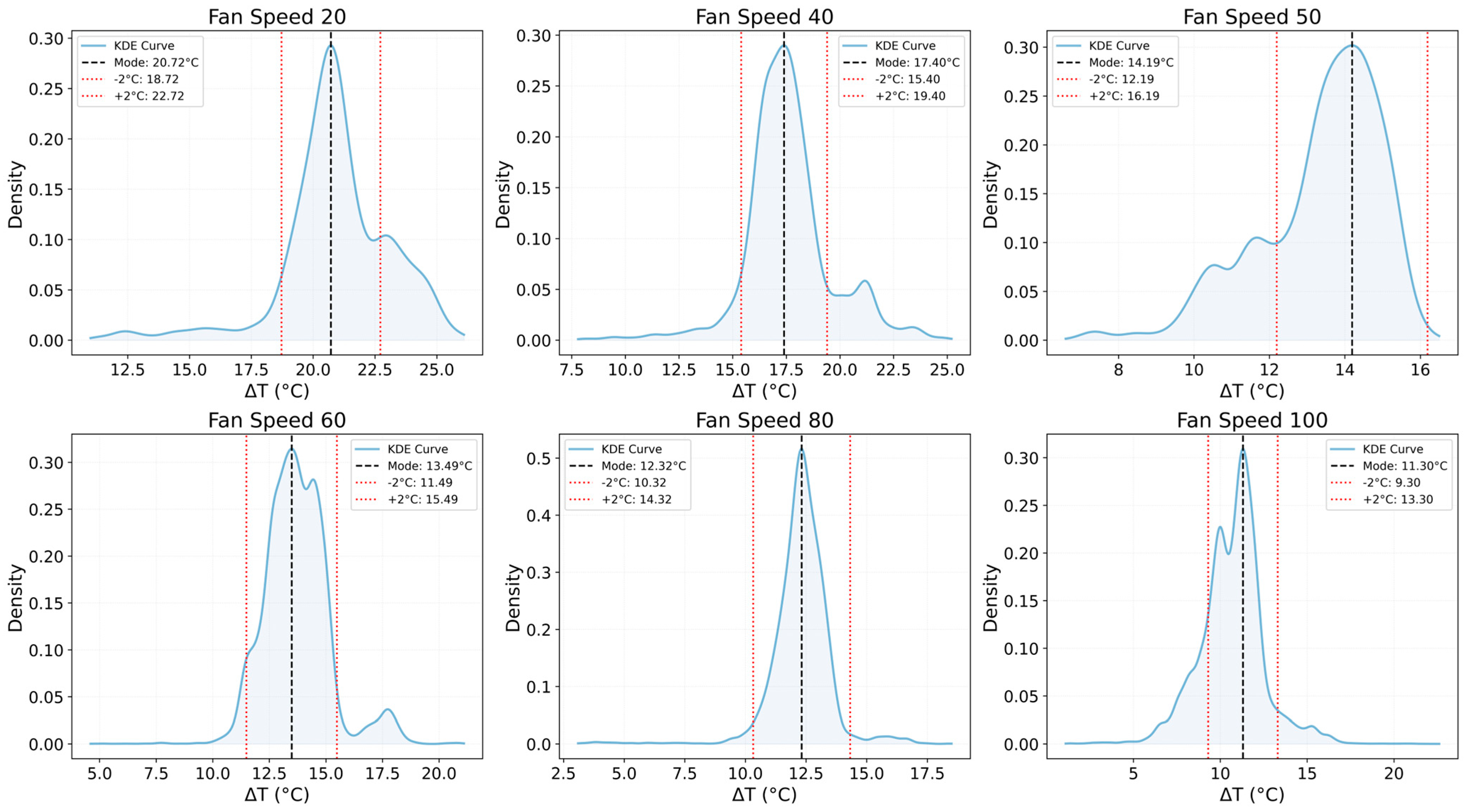
To ensure that only stable operation periods were used for model development, a Kernel Density Estimation (KDE)–based steady-state identification method was applied to the indoor air temperature difference (ΔT) at each fan-speed level. For every airflow condition, the air-side temperature difference between the inlet and outlet exhibited a relatively stable range during continuous operation, typically within a 4 °C span. Within this range, ΔT gradually fluctuated with minor variations due to small load changes or sensor noise, but the overall distribution consistently concentrated around a single dominant peak. This peak represents the most frequent ΔT value, corresponding to the period of prolonged steady-state operation in which both the compressor and the indoor fan maintained stable thermodynamic behavior.
Based on this observation, the mode of the KDE distribution was identified as the representative ΔT for each fan-speed condition, and a stability band of ±2 °C around the mode was defined. This band reflects the empirical finding that the difference between the maximum and minimum ΔT during stable operation seldom exceeded 4 °C. Data falling outside the ±2 °C range were regarded as transient or non-steady conditions, typically caused by events such as door openings, sudden airflow changes, or short-term control adjustments. Consequently, the KDE-based approach effectively isolates the most statistically dominant and physically stable data region, ensuring that only steady-state measurements, representative of sustained system behavior, are retained for regression analysis.
Figure 2 presents the KDE distributions of ΔT for each fan-speed level. The shaded areas denote the ±2 °C stability bands around the KDE modes, confirming that steady-state operation corresponds to the high-density region, whereas the tails of the distribution represent transient deviations.
6.
Step 6. Stable cooling capacities (≤115% of rated value)
ASHRAE Standard 37 [36] stipulates that reported cooling capacities must remain within the rated design envelope. In practice, however, many DX cooling systems are designed to exceed their rated capacities under certain conditions or for short durations. Manufacturer submittal data and independent experimental studies have confirmed this phenomenon. For instance, Mitsubishi, Daikin, and LG single-split systems have been reported to deliver 115–125% of their rated capacities [46,47,48]. Field and laboratory studies on variable-capacity heat pumps have also shown extended operating ranges down to 40% part load and peak capacities of 118–120% of rated [49,50].
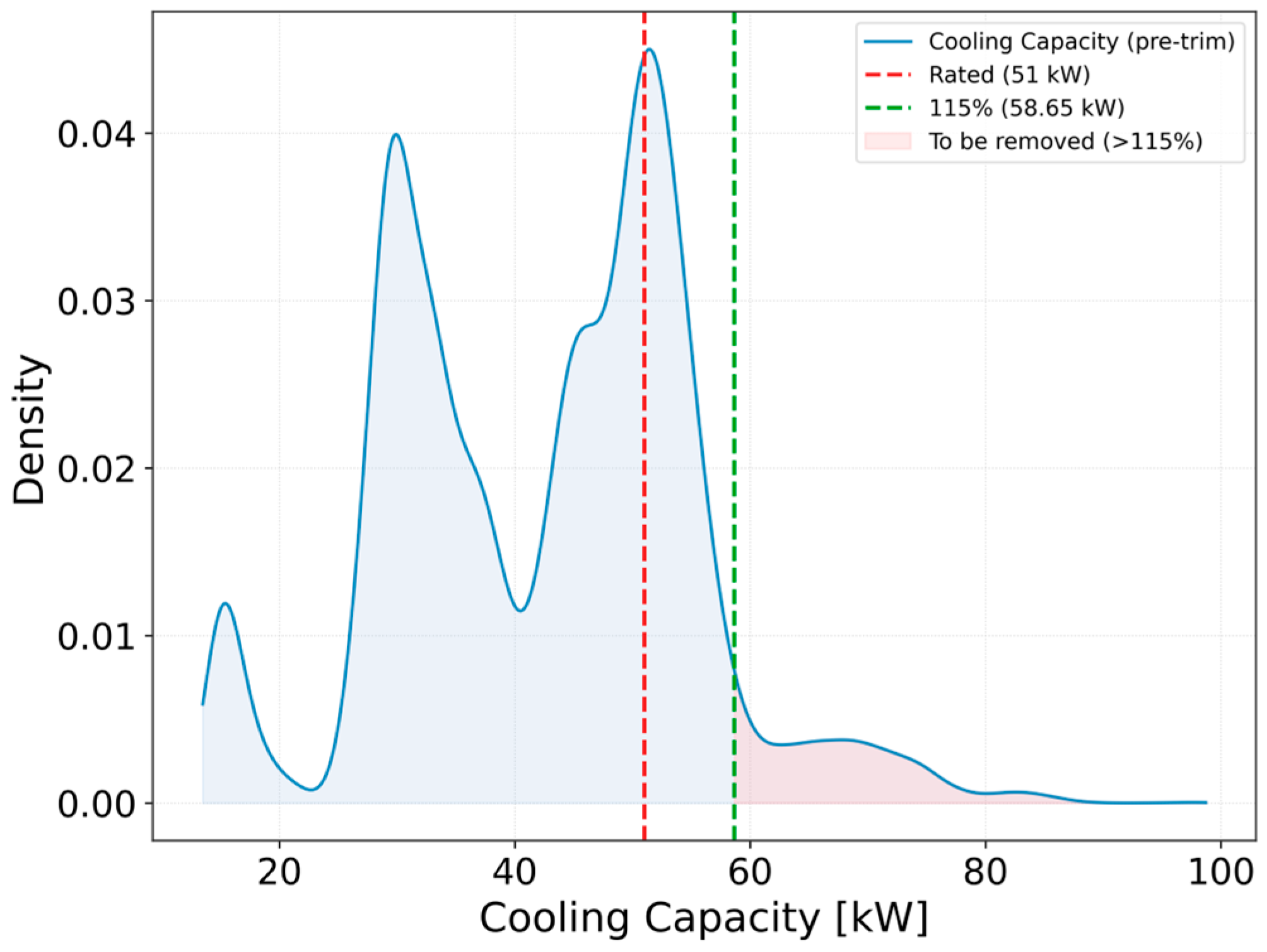
In this study, 115% of rated cooling capacity was conservatively adopted as a universal threshold across equipment types. Data exceeding this limit were considered to represent sensor errors, unstable conditions, or extreme outliers, and were excluded. For reproducibility, it is recommended that if a manufacturer’s catalog specifies a maximum capacity, that value should be used instead of the conventional 115% threshold. This dual approach allows for broad applicability to various DX systems while maintaining consistency with manufacturer-certified performance envelopes. Figure 3 presents the measured cooling capacity distribution with the rated value and the 115% threshold, clearly showing the range and pattern of excluded data. This demonstrates that physically implausible operating points were removed, and the dataset retained only valid steady-state conditions.
Figure 3 illustrates the baseline lines for rated cooling capacity and maximum cooling capacity, along with the data points identified for exclusion.

2.4. Data Splitting for Training and Validation

In this study, the entire dataset was divided into training and validation sets to evaluate the generalization performance of the regression models. Following the common practice adopted in previous studies [51,52], the dataset was split into 80% for training and 20% for validation. A total of 80% of the data was used to derive the regression equations, while the remaining 20% was used for model validation.
Random sampling was applied for data partitioning, while ensuring that samples were evenly extracted within the same operating condition ranges to maintain representativeness. This procedure helped prevent overfitting of the regression models and allowed for a reliable assessment of predictive performance under diverse operating conditions.
Figure 4 presents the distributions of the major independent variables for the training and validation datasets, confirming that both subsets maintained similar distributions.

2.5. Selection of Variables

This section reviews the definitions and physical validity of the main independent variables used in the regression analysis and presents their distributions and combinations. In doing so, it provides the rationale for selecting variables that are not only statistically meaningful but also practically applicable to the operation and control of large-space cooling systems.

2.5.1. Selection and Rationale of Variables

The variables employed in the dataset were defined as follows. The evaporator air-side inlet temperature was defined as indoor temperature (Tin), and the evaporator air-side inlet humidity ratio was defined as indoor humidity ratio (win). The condenser air-side inlet temperature was defined as outdoor temperature (Tout), while the supply airflow rate ( V ˙ ) represented the airflow determined by the indoor unit’s fan speed control. The dependent variable was cooling capacity ( Q ˙ c), calculated based on the air-side enthalpy difference.
The selection criteria for candidate predictors of cooling capacity were based on thermal environmental conditions observable during the actual operation of large-space cooling systems and controllable input parameters. Accordingly, indoor air temperature, outdoor air temperature, indoor humidity, and airflow rate were adopted as independent variables.
Indoor and outdoor temperatures are key factors determining the thermal load of large spaces, and numerous previous studies have repeatedly reported that outdoor temperature and the temperature difference between indoor and outdoor air are primary predictors of cooling demand and energy consumption [25,30].
Indoor humidity was also considered a valid predictor since it reflects the contribution of latent loads and is inherently included in the overall calculation of cooling capacity. Between relative humidity and humidity ratio, the latter was selected, as relative humidity is influenced by temperature and thus provides limited prediction accuracy as an independent variable. Therefore, the humidity ratio was adopted, as it directly represents the moisture content of air independent of temperature.
Airflow rate was included as a controllable input variable. Comparative studies between VAV and VRF systems have demonstrated that differences in control strategies (e.g., airflow modulation and capacity control) exert significant influence on cooling energy performance [6,7]. Furthermore, airflow rate is expected to play a critical role as a future control variable, supporting its inclusion as a predictor.
Although refrigerant mass flow rate and power consumption are strongly correlated with cooling capacity, they were excluded from the input variables because they represent outcome variables rather than operating conditions. Their inclusion would introduce dependency with the target variable, which contradicts the objective of developing a simple and physically interpretable regression model in this study.

2.5.2. Key Independent Variables

In this section, the distribution characteristics of the main input variables adopted in this study were examined.
1.
Indoor temperature (Tin, °C)
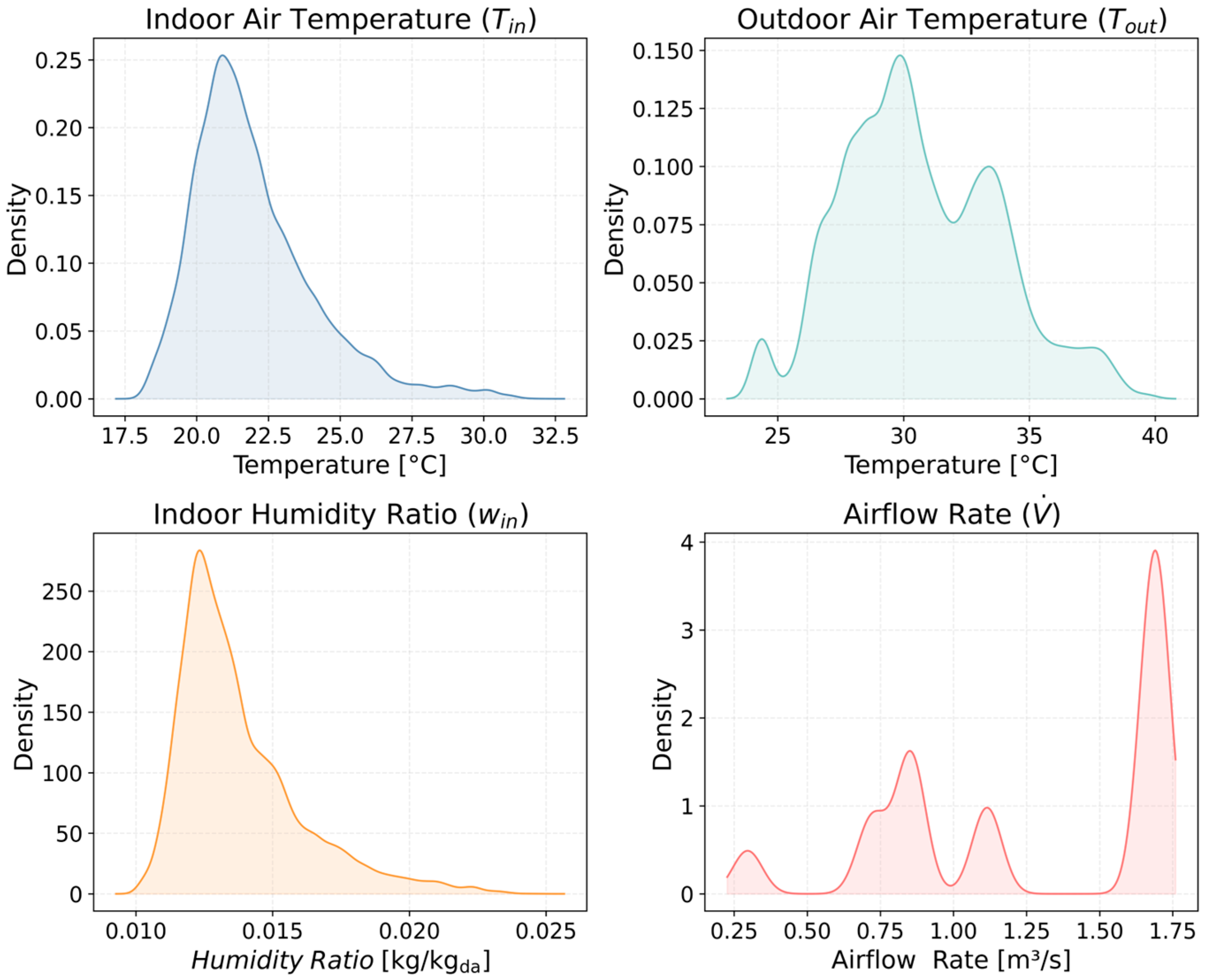
The indoor temperature ranged from 18 to 32 °C, with concentrations observed between 20 and 25 °C and a distinct peak near 21 °C. This corresponds well to the control temperature range of large-space cooling equipment and reflects the fact that the indoor temperature rapidly decreased to the target range and was stably maintained during operation. Such a distribution characteristic indicates that the dataset in this study adequately represents practical cooling operation conditions.
2.
Outdoor temperature (Tout, °C)
The outdoor temperature ranged from 23 to 42 °C, with a concentrated distribution between 28 and 34 °C and a distinct peak near 30 °C. This corresponds to typical summer peak cooling load conditions, suggesting that the dataset is well-suited for performance prediction under varying outdoor environments.
3.
Indoor humidity ratio (win, kg/kgda)
The distribution of the indoor humidity ratio exhibited a pronounced peak in the range of approximately 0.010–0.015 kg/kgda, reflecting the significant moisture content of the indoor air under summer conditions. This feature highlights the importance of considering latent loads in predicting the performance of large-space cooling systems. Unlike relative humidity, the humidity ratio directly quantifies the absolute water vapor content in the air, thereby providing a more consistent and physically interpretable variable. The skewed distribution indicates the influence of the hot and humid summer climate in Korea as well as the experimental conditions, where complete dehumidification was not achieved due to prolonged operation and additional outdoor air infiltration caused by open doors. Accordingly, employing humidity ratio as a predictor strengthens the physical interpretability of the regression model, particularly in capturing latent effects beyond sensible-only models.
4.
Airflow rate ( V ˙ , m3/s)
Airflow distribution was not uniform, showing distinct peaks near 0.5 m3/s and 1.6 m3/s. This reflects the discrete fan speed control characteristic of the system, demonstrating that the unit operates in segmented modes rather than continuous modulation. Airflow thus functions as an important variable representing both control strategy and performance characteristics.
Figure 5 presents the distribution characteristics of the four main variables described above.

2.5.3. Variable Combinations

In this study, regression models were developed using various combinations of the four selected variables. The combinations ranged from single-variable to multivariable models, allowing systematic comparison between simple minimal-variable models and higher-dimensional multivariate models. Table 4 summarizes the variable combinations considered.
As summarized above, this study ultimately selected indoor temperature, outdoor temperature, indoor humidity, and airflow rate as the key independent variables to construct regression models that are both physically interpretable and parsimonious. This selection not only ensures statistical adequacy but also provides practical applicability for future control strategies and energy-saving measures. Among the candidate models, the focus was placed on deriving minimal-variable regression equations that can effectively support performance analysis, control applications, and energy conservation.

2.6. Regression Analysis and Validation Method

In this study, regression analysis techniques were applied to predict the cooling capacity of the system. To derive the most suitable regression equations, a range of approaches was examined, including linear, polynomial, and nonlinear regression (e.g., rational function-based models). All regression analyses were implemented in the Python 3.13 (Python Software Foundation, Wilmington, DE, USA) nvironment. Linear and polynomial regressions were performed using scikit-learn library, whereas nonlinear regression was conducted with the SciPy packages (curve_fit, least_squares). Data handling and numerical operations employed NumPy and Pandas, and the results were organized with OpenPyXL (open-source community) and python-docx (open-source community).

2.6.1. Regression Models Considered

To quantitatively predict the cooling capacity of the modular vertical DX cooling system, various regression methods were applied in a stepwise manner. First, simple linear regression (SLR) was performed to identify the primary relationships between each independent variable and the dependent variable, thereby clarifying the individual effects of input variables. Subsequently, multiple linear regression (MLR) was used to evaluate the combined influence of indoor temperature, outdoor temperature, airflow rate, and indoor humidity on cooling capacity.
Polynomial regression was introduced to account for nonlinear effects and interaction terms between variables. Second-order terms and cross-terms were included to enhance prediction accuracy, while higher-order terms were avoided to maintain model simplicity and reduce the risk of overfitting.
In addition, since the thermodynamic behavior of air-conditioning systems is often not adequately described by simple linear relationships, nonlinear regression models were tested. Specifically, functional forms such as 1/Tout and ln (Tout) were employed to reflect the refrigerant cycle characteristics and condenser heat transfer behavior, thereby capturing the diminishing performance trend under rising outdoor temperatures more realistically.
Table 5 summarizes the regression models considered in this study, including their mathematical forms and key features.

2.6.2. Evaluation Metrics

To evaluate the performance of the regression models, four major metrics were selected: the coefficient of determination (R2), the adjusted coefficient of determination (Adj R2), the root mean square error (RMSE), and the mean absolute error (MAE). These indicators have been widely applied in previous studies on building energy performance prediction. For instance, Sadeghi et al. evaluated the performance of residential buildings using R2, RMSE, and MAE [17], while Wefki et al. employed R2 and RMSE to quantitatively validate model accuracy [53]. The adjusted R2 was additionally introduced to correct the upward bias of R2 when the number of independent variables increases.
First, the coefficient of determination (R2) indicates how much of the variance in the dependent variable is accounted for by the model. The value ranges from 0 to 1, and values closer to 1 represent stronger predictive capability. It is calculated according to Equation (8). In this expression, y i denotes the observed value, y ^ i is the predicted value, y ¯ is the mean of observed values, and n is the number of samples.
R 2 = 1 i = 1 n ( y i y ^ i ) 2 i = 1 n ( y i y ¯ ) 2
Second, the adjusted coefficient of determination (Adj R2) accounts for the tendency of R2 to increase as more independent variables are added, even when they provide little contribution to the model. It provides a more reliable measure of model generalization, particularly against overfitting. The formula is given in Equation (9), where n is the sample size and p is the number of independent variables.
A d j   R 2 = 1 ( 1 R 2 ) n 1 n p 1
Third, the root mean square error (RMSE) quantifies the overall magnitude of the prediction error. It is obtained by squaring the differences between observed and predicted values, averaging them, and then taking the square root. Smaller RMSE values indicate higher predictive accuracy. The calculation is shown in Equation (10).
R M S E = 1 n i = 1 n ( y i y ^ i ) 2
Fourth, the mean absolute error (MAE) represents the average absolute difference between predicted and observed values. This metric is more straightforward to interpret and less sensitive to outliers than RMSE. It is defined in Equation (11).
M A E = 1 n i = 1 n | y i y ^ i |
Together, these metrics provided a comprehensive framework for evaluating model performance. R2 and Adj R2 were used to assess prediction accuracy, RMSE quantified the absolute magnitude of prediction errors, and MAE offered complementary insight by indicating the stability of the dataset and the effect of outliers. Through this multi-faceted validation, the performance of the proposed regression models was comprehensively assessed.

2.6.3. Validation of Regression Models

The regression models that were finally considered suitable were validated using the 20% test dataset separated in advance. Predicted values were compared with observed values in order to examine potential overfitting and to verify whether predictive performance was maintained under actual operating conditions.
The evaluation metrics applied were the R2 and the RMSE, which were primarily used in the regression analysis. In addition, the MAE was employed to assess model stability and sensitivity to outliers.
To visually examine the agreement between predicted and observed values, three graphical methods were used. First, scatter plots of predicted versus observed values were drawn, where data points closer to the y = x line indicated better model fit. Second, residual plots were examined. When the residuals were evenly distributed around zero, the assumption of homoscedasticity was met, indicating that the regression model was statistically valid. Third, quantile–quantile (QQ) plots of residuals were analyzed. If the residuals followed a normal distribution, the points aligned along the diagonal line, thereby confirming the normality assumption of regression analysis.
Through the combined use of numerical metrics and graphical diagnostics, the generalization capability and reliability of the proposed regression models were comprehensively evaluated.

3. Results

A total of 46 regression models were derived by systematically expanding the selected variable combinations, as shown in Appendix A Table A3. In the main text, the results are presented with a focus on representative models that satisfy both statistical significance and physical interpretability. The analytical flow proceeds from an initial review of univariate models, followed by a comparison of multivariate models with higher accuracy, and concludes with validation of the final regression equation. Univariate regression is particularly useful as a starting point for assessing the individual contribution of each variable, but in practice, most results showed low accuracy, confirming the necessity of multivariate analysis. The final model was selected based on a balance between simplicity, physical consistency, and predictive performance, and detailed interpretations are presented in this chapter, while the overall evaluation and research implications are synthesized in the Discussion.

3.1. Influence of Individual Variables

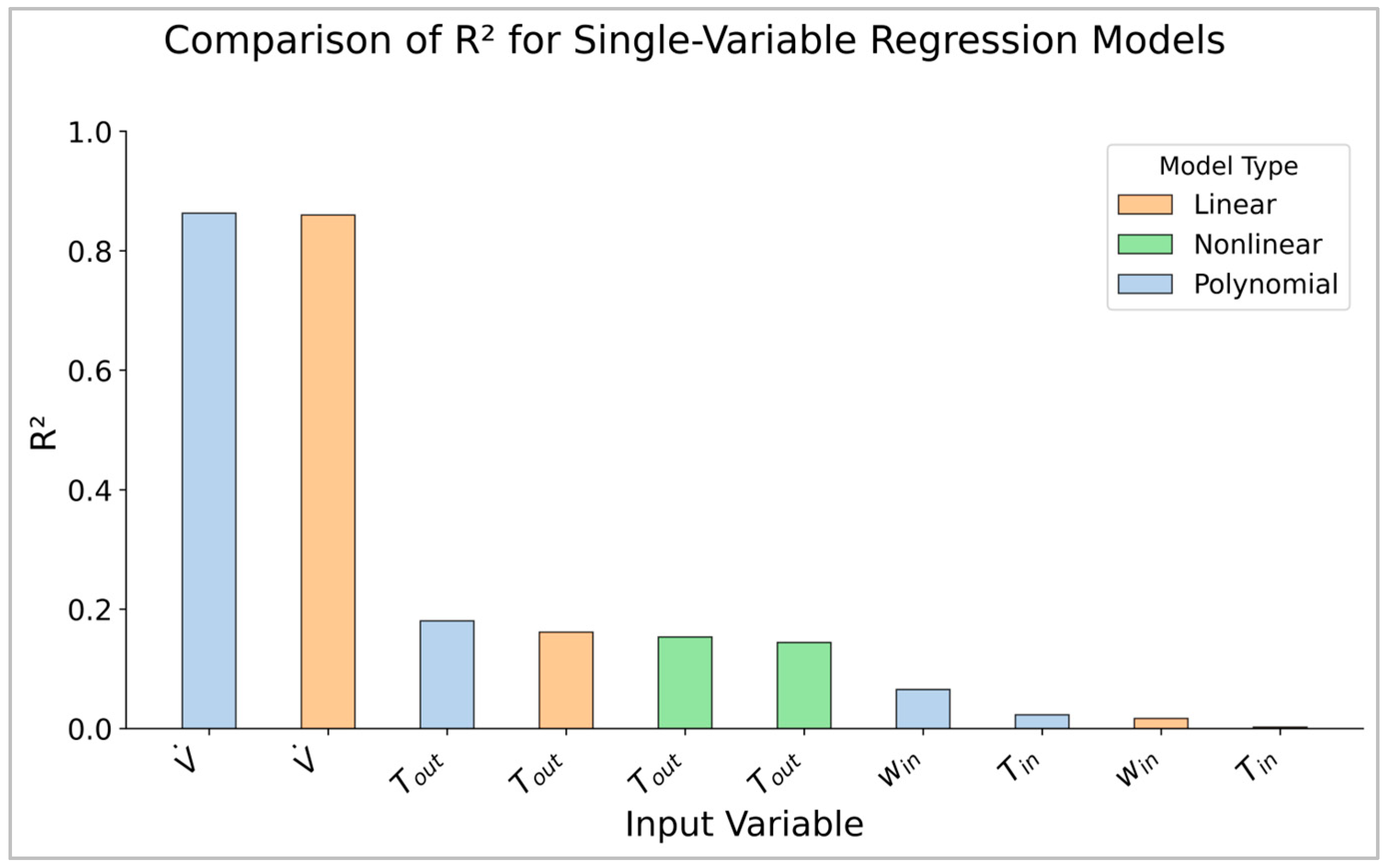
Figure 6 compares the prediction accuracy (R2) of single-variable regressions. Among all candidates, airflow rate ( V ˙ ) shows a clearly dominant, near-linear relationship with cooling capacity, reaching R2 ≈ 0.86. The polynomial form only marginally improves R2 over the linear fit, which corroborates the physical expectation that Q ˙ c m ˙ Δh and that m ˙ scales with V ˙ on the air side; thus, the capacity increase with airflow is essentially linear within the observed envelope.
By contrast, outdoor temperature (Tout) alone offers limited prediction accuracy (R2 ≤ 0.18), and even yields a positive linear coefficient in the single-variable fit. This pattern reflects control compensation, in example, inverter-driven compressor speed and EEV modulation, which partially offsets condenser-side degradation as Tout rises; the net effect weakens the apparent marginal influence of Tout in a purely univariate view. Nonlinear forms (ln Tout, 1/Tout) bring only slight R2 gains, consistent with a gentle curvature of performance with outdoor conditions rather than a strong nonlinearity.
Indoor humidity ratio (win) and indoor temperature (Tin) show very low univariate R2 (≈0.017 and ≈0.023, respectively). For win, incomplete dehumidification and door-opening infiltration during field operation likely reduced variance, limiting its standalone predictive value. For Tin, covariance with other drivers (e.g., Tout, V ˙ ) obscures its isolated effect; accordingly, its role should be reassessed in multivariate contexts rather than judged only by single-variable fits.
Physical interpretation and implications:
(1)
The air-side mass-flow term governs capacity most strongly in our dataset, so V ˙ is the principal control-oriented predictor. This aligns with the enthalpy-difference formulation and the observed near-linearity of V ˙ Q ˙ c relations.
(2)
The outdoor-temperature effect exists physically (capacity tends to decline with higher Tout), but on-board compensation flattens the univariate trend; hence Tout contributes more as a moderating/interaction variable than as a lone predictor.
(3)
Although the univariate R2 of Tin is small, it remains operationally critical: it reflects the current indoor state and serves as the primary control target/setpoint for capacity delivery. Thus, Tin must be retained in minimal practical models and in any control discussion, even if its isolated statistical contribution appears small in a univariate screen.
(4)
win can be treated as supplementary: it helps interpret latent-load conditions and tail behaviors, but is not essential for a compact, control-ready baseline.

3.2. Review of Models with High Prediction Accuracy (R2 > 0.90)

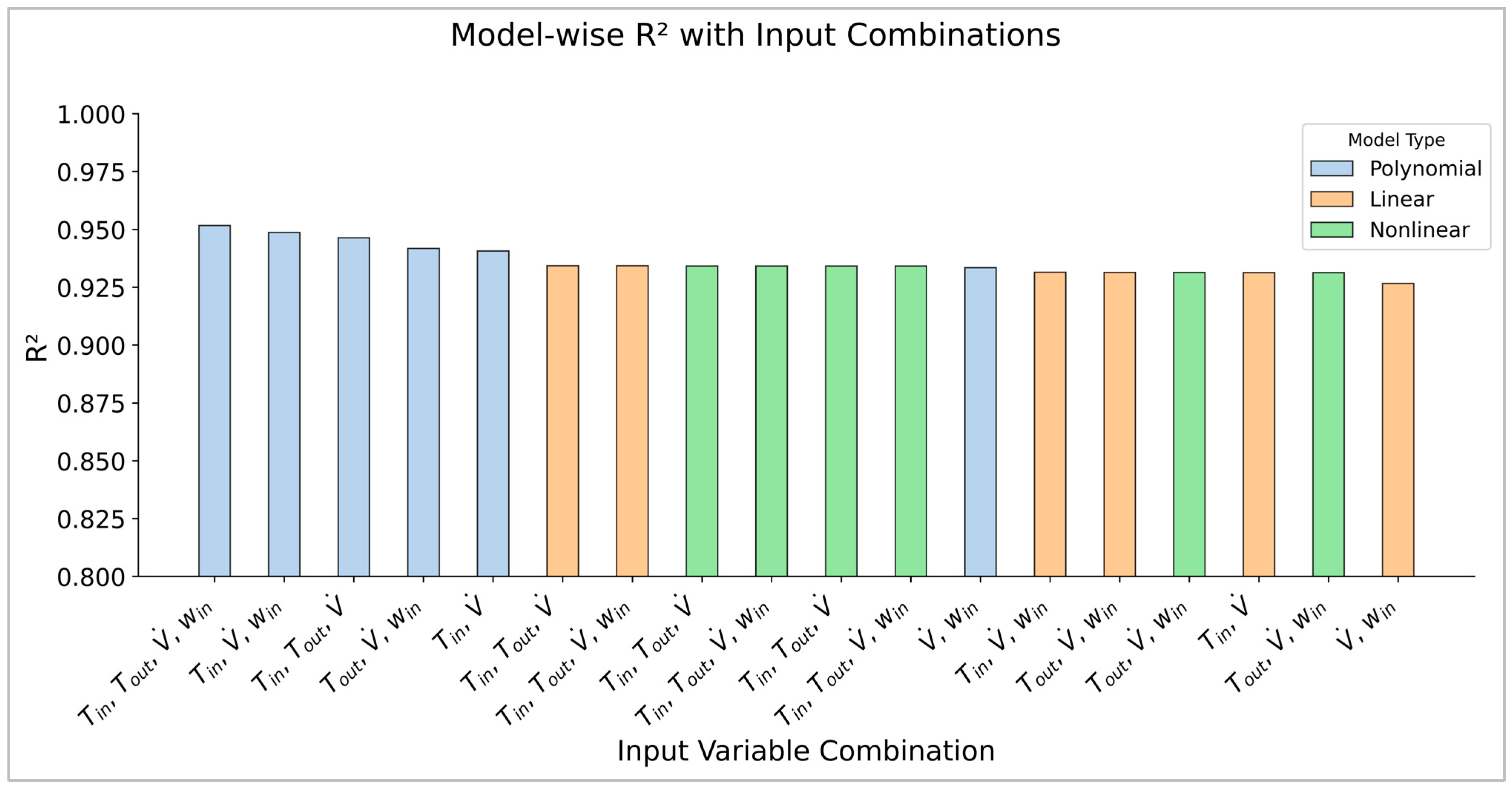
Figure 7 compares the R2 values of multivariable regression models employing different combinations of input variables. Overall, polynomial regressions exhibited slightly higher R2 values than linear and nonlinear ones, suggesting that interaction terms such as Tin· V ˙ and Tout· V ˙ may have a meaningful effect on predicting cooling capacity. This implies the existence of cross-variable interactions, where indoor load and airflow jointly influence the heat transfer rate and the resultant cooling capacity.
Physically, these cross-terms represent the coupled behavior between indoor air temperature and airflow control. An increase in airflow enhances convective heat transfer on the indoor heat exchanger surface, which mitigates the capacity degradation caused by higher outdoor air temperature. Similarly, the interaction between Tin and V ˙ reflects the combined influence of indoor thermal load and air supply rate. Under higher load conditions, greater airflow is required to maintain cooling equilibrium. Therefore, the slightly superior performance of polynomial regression indicates that the system exhibits mild nonlinear coupling between variables.
However, the improvement in accuracy from polynomial models was marginal (ΔR2 < 0.02). This demonstrates that linear regression models can already capture the dominant physical relationships with sufficient accuracy (R2 ≈ 0.94–0.95). Such results confirm that complex polynomial structures do not necessarily provide practical advantages for prediction or control purposes.
Consequently, a three-variable linear regression model using Tin, Tout, and V ˙ was identified as the most suitable model that fulfills the objectives of this study. The model is presented in Equation (12).
Q ˙ c = 26.02 + 1.41 · T i n + 0.21 · T o u t + 23.31 · V ˙
This model offers a balance between simplicity and physical interpretability: it reduces mathematical complexity, provides coefficients that can be directly linked to thermodynamic behavior, and requires only three measurable variables, enabling straightforward implementation in both prediction and control frameworks. By minimizing sensor dependency while maintaining high predictive performance, this approach enhances the model’s practical applicability to real-time HVAC operation.
Although additional models incorporating the indoor humidity ratio (win) were also tested, the improvement in predictive accuracy was marginal (ΔR2 < 0.02). This limited contribution of win is attributed to the fact that the experimental operating envelope maintained a nearly constant sensible heat ratio (SHR). Under such conditions, latent cooling is proportionally linked to sensible cooling, meaning that its effect is already reflected through temperature-related variables (Tin) and airflow ( V ˙ ), rather than acting as an independent factor. Consequently, win provides redundant information instead of introducing a new explanatory variable, resulting in only minor statistical enhancement while increasing model complexity. Therefore, the three-variable formulation was retained as the representative model, balancing simplicity, interpretability, and practical applicability.
In summary, while polynomial regression highlights the presence of mild variable interactions, the three-variable linear regression model was determined to be the most suitable representative due to its simplicity, interpretability, and near-equivalent accuracy. In the following section, this selected model will be validated against measured data to confirm its robustness and to examine the physical meaning of each coefficient, particularly the outdoor temperature term (Tout), and to investigate how it affects overall system performance.
Furthermore, this model will also be employed to analyze COP behavior and to discuss its potential applicability to control strategies.

3.3. Physical Interpretation of the Coefficient

Each coefficient in Equation (12) represents the physical sensitivity of the cooling capacity to its corresponding variable under steady-state operation. The relative magnitudes and signs of these coefficients can be directly associated with the thermodynamic characteristics of the system.
The coefficient of Tin (+1.41) indicate that the cooling capacity increases with higher indoor temperature. This reflects the sensible-load effect, in which a larger temperature difference across the evaporator enhances the air-side heat transfer rate. Although its absolute influence is smaller than that of airflow, Tin expresses the system’s adaptive response to indoor load variations and represents the control variable that drives the system toward the setpoint.
The coefficient of V ˙ (+23.31) is the largest among the three predictors, confirming that air-side mass flow is the dominant factor determining cooling capacity. The nearly linear dependence of Q ˙ c on V ˙ is consistent with the enthalpy-difference formulation ( Q ˙ c = m ˙ air·Δh, with m ˙ air V ˙ ). This large coefficient quantifies the strong controllability of capacity via fan-speed modulation and highlights that most of the system output adjustment is achieved through airflow variation rather than temperature change.
The coefficient of Tout (+0.21) appears positive, contrary to the usual expectation that cooling performance decreases with increasing outdoor temperature. This pattern arises because field operation involves compensatory control responses, mainly compressor speed and refrigerant-flow adjustments, that partially offset condenser degradation at high ambient temperatures. Consequently, the steady-state dataset exhibits an apparent slight increase in capacity with Tout, even though the intrinsic thermodynamic tendency remains negative. When nonlinear transformations such as ln Tout or 1/Tout are applied, the expected gradual decline reappears, in agreement with physical behavior.
Figure 8 compares the linear and nonlinear representations, showing that the nonlinear model reproduces the moderate reduction in cooling capacity at elevated outdoor temperatures.
Overall, the comparison among coefficients shows the following order of influence: β_ V ˙ ≫ β_Tin > β_Tout. Airflow dominates as the principal controllable factor, Tin reflects internal load conditions, and Tout serves as a secondary correction variable preserving physical consistency across ambient environments. Equation (12) therefore encapsulates the balanced interaction between air-side capacity scaling, indoor load compensation, and outdoor-condition moderation, providing a concise yet physically interpretable description of the system’s cooling behavior.

3.4. Validation of the Prediction Model

As confirmed in Section 3.2, the multiple linear regression model, Equation (12), using indoor temperature (Tin), outdoor temperature (Tout), and airflow rate ( V ˙ ) best fulfills the objectives of this study. In this section, the model is further validated to confirm its prediction accuracy.
The performance of this model was evaluated using an independent validation dataset, as summarized in Table 6. The validation results showed that the coefficient of determination (R2 = 0.9341) was nearly identical to that of the training dataset (R2 = 0.9343). Both RMSE and MAE also exhibited comparable values, confirming the stable generalization ability of the model.
Under near-rated conditions (Tout = 34–36 °C, 100% airflow), the measured cooling capacity averaged 52.3 kW.
To evaluate the model accuracy relative to the measured data, the relative error was calculated based on the measured cooling capacity near the rated condition, as expressed by Equation (13).
R e l a t i v e   E r r o r   % = R M S E Q m e a s u r e d × 100
Based on the validation results, the RMSE and mean predicted capacity were 2.86 kW and 52.3 kW, respectively, yielding a relative error of approximately 5.5%.
This indicates that the predicted cooling capacities deviate from the model’s fitted trend by less than ±6% on average, confirming the strong predictive reliability of the proposed regression model.
To further validate the adequacy of the model, three diagnostic plots were examined, namely, the predicted versus observed (parity) plot, the residuals versus fitted values, and the normal QQ-plot in Figure 9.
The parity plot shows a narrow band of data points densely concentrated along the 1:1 reference line, indicating that the predicted capacities closely match the observed ones throughout the full operating envelope. No systematic deviation is observed at either low or high Q ˙ c, suggesting that the model achieves high predictive accuracy without underestimation or overestimation in any capacity range. The slope of the fitted line visually approaches unity and the intercept is close to zero, confirming that there is negligible bias in calibration transfer from the training to the validation dataset.
The residuals versus fitted plot exhibits a symmetric, random cloud of points centered around zero without discernible curvature or funneling patterns. This indicates that the linear model sufficiently captures the dominant physical relationships among Tin, Tout, and V ˙ , while maintaining approximately constant variance of errors (i.e., no evidence of heteroscedasticity). Importantly, no residual clustering or structural breaks are observed near operating points corresponding to high airflow or extreme outdoor temperature, implying that control-induced operating transitions do not introduce bias into the model.
The normal QQ-plot further confirms the distributional adequacy of the residuals. The residual quantiles align closely with the 45° reference line across most of the distribution, with only slight departures at the tails, which are typical for field-collected HVAC data. This behavior suggests that the errors are approximately normal and centered around zero, validating the use of standard regression-based uncertainty measures.
Taken together, these three diagnostic plots verify that the selected three-variable linear regression model (Equation (12)) satisfies the fundamental assumptions of linear regression, including unbiasedness, approximate normality, and homoscedasticity. Moreover, the consistent pattern across different operating regimes demonstrates that the model maintains stable predictive performance and can therefore be considered sufficiently robust for further analyses such as coefficient interpretation, COP evaluation, and control-oriented applications.
Furthermore, comparative validation was conducted with models incorporating higher-order nonlinear terms. Figure 10 presents the QQ-plots of residuals for the linear model, the rational model (1/Tout), and the extended nonlinear model with second-order and interaction terms. All three models showed that residuals closely followed the normal distribution, particularly around the center of the distribution. While the nonlinear models exhibited slight improvements in the tail regions, the overall distribution characteristics were not substantially different from those of the linear model, and no significant improvement in predictive accuracy was observed. This indicates that introducing additional higher-order terms does not meaningfully enhance the prediction accuracy of the model.
Therefore, considering simplicity, physical interpretability, and applicability to various equipment and outdoor conditions, the three-variable linear regression model (Equation (12)) was determined as the final model. This choice eliminates unnecessary complexity while ensuring sufficient predictive capability. From an academic perspective, it highlights the feasibility of achieving accurate prediction with minimal variables, and from a practical perspective, it provides significant value for direct application to system control and design.

3.5. Analysis of the Coefficient of Performance (COP)

As discussed in the previous section, although the increase in outdoor temperature can be partially compensated by control interventions in terms of cooling capacity, different results may appear in terms of efficiency. To examine this, the coefficient of performance (COP), a representative indicator of cooling performance, was analyzed. COP is generally calculated according to the test conditions specified in ASHRAE Standard 37 [36], and the present study referred to operating conditions that closely matched this standard.
Field data were collected under random operating conditions. However, due to missing power consumption data, it was not possible to calculate COP directly across the entire dataset. Therefore, the COP analysis was performed by selecting the conditions most similar to the standard COP calculation conditions from the available dataset. The accuracy of the power prediction model was relatively low, with an R2 value of 0.3546 in the linear regression model and a modest improvement to R2 = 0.4378 in the second-order polynomial model. Accordingly, the second-order polynomial model was applied for power prediction, which was then combined with the cooling capacity regression model (Equation (12)) to estimate COP. COP was calculated as the ratio of predicted cooling capacity to predicted power consumption, as shown in Equation (14).
C O P m o d e l = Q ^ c P ^
The analysis results are summarized in Table 7. Under the same operating conditions, the measured COP was 4.2, while the predicted COP was 3.5, yielding a difference of approximately 0.7. This discrepancy is attributed to the relatively low accuracy of the power prediction model. Nevertheless, the predicted results indicated that COP values were 3.5, 3.2, and 3.1 at outdoor temperatures of 28.8 °C, 35 °C, and 40 °C, respectively, confirming a gradual decrease in COP as outdoor temperature increased.
This result clearly demonstrates that while cooling capacity can be partially maintained under rising outdoor temperatures through compensatory control, such compensation requires higher power input, leading to a gradual decline in COP. Although the absolute accuracy is limited by the constraints of the available power data, the analysis confirms the physical tendency that increasing outdoor temperature results in lower COP. Therefore, the COP analysis provides supplementary evidence to the earlier conclusion that the outdoor temperature variable must be considered not only in relation to cooling capacity but also in terms of system efficiency.

4. Discussion

The present study demonstrates that a physically interpretable regression model with only three measurable variables, indoor temperature (Tin), outdoor temperature (Tout), and airflow rate ( V ˙ ), can effectively predict the cooling performance of a large-space modular DX system under field conditions. This result is particularly meaningful considering that most previous studies have relied on complex AI or hybrid frameworks involving numerous variables and extensive preprocessing to achieve similar levels of accuracy. The proposed approach thereby highlights that a minimal-variable, physically consistent formulation can achieve sufficient accuracy while maintaining transparency and practical usability for real-time control.

4.1. Physical Interpretation and Model Behavior

The developed linear regression equation quantitatively captures the essential thermodynamic dependencies of cooling performance. The positive coefficient of Tout implies the compensatory behavior of the compressor and expansion valve when outdoor temperature rises, while Tin acts as a proxy for the internal sensible load. Among the independent variables, airflow rate ( V ˙ ) shows the strongest influence, confirming that air-side heat transfer is the dominant factor governing total capacity scaling. These relationships align with the physical principles of direct expansion cooling and validate that the model not only achieves numerical accuracy but also preserves physical interpretability. Nonlinear and polynomial alternatives tested during this study produced marginal accuracy improvements (ΔR2 < 0.02), indicating that the intrinsic linearity between the selected variables sufficiently explains the observed system behavior within the rated envelope.

4.2. Comparison with AI-Based Models

Recent studies employing artificial intelligence have achieved remarkable predictive accuracy in HVAC applications. Deep neural networks, Gaussian Process Regression (GPR), and PSO-optimized LSSVM models frequently report R2 values above 0.95, supported by complex input sets and multi-layer nonlinear mappings. However, such models often require extensive datasets, repeated training, and hyperparameter tuning, which limit their practical applicability in real-time supervisory control. Moreover, their internal structures obscure the direct influence of physical parameters, making them unsuitable for control-oriented applications where transparency and sensitivity interpretation are critical.
In contrast, the proposed regression model achieves comparable accuracy (R2 = 0.93) using only three measurable inputs, Tin, Tout, and V ˙ , without the need for iterative optimization or large-scale training. Each coefficient directly quantifies the sensitivity of cooling capacity to its corresponding physical driver, allowing intuitive interpretation and diagnostic use. This characteristic makes the model fundamentally different from ANN or PSO-LSSVM frameworks: it serves not only as a predictor but also as a physically grounded equation usable in airflow modulation, capacity estimation, and supervisory control. While black-box AI models tend to maximize precision, this study demonstrates that interpretability and computational simplicity can coexist with practical levels of predictive fidelity, particularly when applied to large-space DX systems with limited sensing infrastructure.

4.3. Limitations

Although the proposed model shows high consistency and robustness, several limitations remain. First, the power consumption data required for COP analysis were partially incomplete due to logging interruptions during long-term measurement. As a result, an accurate regression model for electrical power could not be established, and the predicted COP was calculated using a secondary polynomial fit derived from incomplete data. Consequently, the absolute difference between measured and predicted COP values must be viewed as an artifact of data deficiency rather than a model inadequacy. Nevertheless, the overall declining trend of COP with increasing outdoor temperature was correctly reproduced, supporting the validity of the proposed framework.
Second, the measurement campaign was designed to capture diverse operating conditions but was not conducted as continuous seasonal monitoring. The dataset therefore included random sampling rather than long-term time-series logging, leading to partial absence of data under specific outdoor humidity or temperature conditions. This restriction limits the model’s generalization to extreme boundary states beyond the observed operating envelope. Despite these constraints, the dataset covers the most frequent real operating range for industrial-type DX systems, ensuring that the regression relationships remain representative for field applications.
Third, the present analysis was confined to a single-unit system to isolate the intrinsic performance relationships. In actual modular installations, multiple units operate in parallel and share loads dynamically through staging and airflow adjustments. Such interactions may introduce system-level nonlinearities not captured in the current unit-based model. Future studies should therefore extend this framework to multi-unit operation and evaluate the integrated control benefits using dynamic simulation and field implementation.
Another limitation stems from the fixed installation of the sensors. Once installed in the testbed, their positions could not be altered without disrupting the experimental environment. Consequently, a sensitivity analysis on sensor placement could not be performed. Nevertheless, the sensors were positioned at locations that best represented the overall airflow and thermal characteristics of the test zone, in accordance with ASHRAE measurement guidelines. For airflow rate measurements, the mean value obtained from the five-point method across the duct cross-section was used to reduce spatial bias and measurement uncertainty. These procedures ensured that the acquired data were as representative and repeatable as possible, despite the absence of an explicit location-sensitivity evaluation.

4.4. Practical and Methodological Implications

The simplicity and interpretability of the proposed regression model provide distinct advantages for control and design practice. Because all inputs correspond to readily available field sensors, the model can be directly embedded in supervisory logic for real-time airflow control, capacity estimation, and energy optimization. Furthermore, its transparent structure allows engineers to understand, adjust, and verify the control behavior without relying on opaque machine-learning models. This interpretability is crucial for industrial applications where operational stability, explainability, and maintenance simplicity are prioritized over marginal gains in statistical accuracy.
Methodologically, this study challenges the prevailing assumption that higher model complexity always leads to superior performance. By demonstrating that a minimal-variable linear regression can deliver predictive fidelity comparable to complex AI-based frameworks, it establishes a practical middle ground between empirical regression and data-driven prediction. This paradigm promotes the broader adoption of interpretable, physics-aligned models that balance accuracy, transparency, and computational efficiency in large-space HVAC analysis and control.

5. Conclusions

This study examined whether a minimal-variable, physically interpretable regression model can achieve predictive accuracy comparable to more complex AI-based approaches while remaining applicable to real-time supervisory control of modular DX systems. To this end, a transparent three-variable framework using only standard measurable inputs was developed and evaluated on field data.
The following conclusions can be drawn:
  • A three-variable linear model consisting of indoor temperature (Tin), outdoor temperature (Tout), and airflow rate ( V ˙ ) achieved R2 ≈ 0.93 on field data; on the independent validation set, R2 = 0.9341, RMSE = 2.86 kW, MAE = 2.31 kW, corresponding to about ±6% deviation near rated conditions.
  • Graphical diagnostics (parity, residuals-vs-fitted, normal QQ) indicate a narrow 1:1 band without systematic bias, approximately normal zero-mean residuals, and no visible heteroscedasticity, supporting model adequacy across the observed envelope.
  • In model form comparison, second-order polynomial and simple nonlinear alternatives (e.g., 1/Tout, ln Tout) yielded only marginal gains (ΔR2 < 0.02), showing that a linear form already captures the dominant relationships among Tin, Tout, and V ˙ .
  • Indoor humidity ratio (win) provided only minor improvement (ΔR2 < 0.02); under the test SHR conditions, latent effects were effectively reflected through temperature-related terms and airflow, making win redundant for a compact baseline model.
  • Coefficient interpretation is physically consistent: capacity scales most strongly with V ˙ ; Tin shows positive sensitivity (indoor load), while Tout’s small apparent effect reflects field control compensation, consistent with the operating envelope.
  • Limitations include partial power-data loss (precluding a robust COP regression), non-season-long sampling (under-representation at extreme humidity/temperature), single-unit testing (no system-level interactions), and fixed sensor placement; nonetheless, the dataset spans frequent real-world operating ranges.
The novelty of this study lies in reversing the prevailing trend toward increasing model complexity. It demonstrates that comparable predictive accuracy can be achieved without nonlinear or hybrid structures, while maintaining superior interpretability, computational simplicity, and physical transparency. By explicitly linking regression coefficients to physical parameters, the model bridges empirical data with thermodynamic understanding, offering both predictive and diagnostic utility.
Future research will focus on extending this framework in two key directions.
First, the proposed regression model will be implemented in a real-time control environment to validate its practical effectiveness under dynamic operation.
Second, multi-unit operation scenarios in large-space modular systems will be examined to evaluate partial-load adaptability, system-level interactions, and the potential for energy savings.
These efforts will further verify the scalability and applicability of the developed framework for advanced control and field deployment.

Author Contributions

Conceptualization, T.U.M.; Methodology, T.U.M.; Experiment, T.U.M.; Software, T.U.M. and Y.I.K.; Verification, Y.I.K.; Formal analysis, T.U.M.; Investigation, T.U.M.; Resources, T.U.M.; Data Curation, T.U.M. and Y.I.K.; Writing—Original draft preparation, T.U.M. and Y.I.K.; Writing—Review and Editing, Y.I.K.; Visualization, T.U.M.; Director, Y.I.K.; Project Management, Y.I.K.; Funding, Y.I.K. All authors have read and agreed to the published version of the manuscript.

Funding

This research received no external funding.

Data Availability Statement

The original contributions presented in the study are included in the article, further inquiries can be directed to the corresponding author.

Conflicts of Interest

The authors declare no conflicts of interest.

Abbreviations

The following abbreviations are used in this manuscript:
Abbreviation
AArea [m2]
Adj R2Adjusted R2
ANNArtificial Neural Network
ASHRAEAmerican Society of Heating Refrigerating and Airconditioning Engineers
BASBeetle Antennae Search algorithm
COPCoefficient of Performance
CNNConvolutional Neural Network
DNNDeep Neural Network
daDry air
DELMDeep Extreme Learning Machine
DOASDedicated Outdoor Air Systems
GAGenetic Algorithm
GPRGaussian Process Regression
GRNNGeneralized Regression Neural Network
HVACHeating, Ventilation, and Air-Conditioning
KDEKernel Density Estimation
IPSOImproved Particle Swarm Optimization
LSSVMLeast Squares Support Vector Machine
LSTMLong Short-Term Memory
MAEMean Absolute Error
MAPEMean Absolute Percentage Error
MLRMultiple Linear Regression
MPCModel Predictive Control
PSO-LSSVMParticle Swarm Optimization–Least Squares Support Vector Machine
R2Coefficient of determination
RMSERoot Mean Squared Error
SLRSimple Linear Regression
SSASingular Spectrum Analysis
VAVVariable Air Volume
VRFVariable Refrigerant Flow
XGBExtreme Gradient Boost
Nomenclature
c p Specific heat at constant pressure [kJ/kg·K]
m ˙ Mass flow rate [kg/s]
ρ Density [kg/m3]
Q ˙ c Cooling capacity [kW]
Q l a t Latent heat [kW]
Q s e n s Sensible heat [kW]
Q t o t Total heat [kW]
T i n Indoor unit evaporator inlet temperature [°C] = Indoor temperature
T o u t Indoor unit evaporator outlet temperature [°C]
T Temperature difference
V ˙ Indoor unit airflow rate (volumetric flow rate) [m3/s]
w i n Indoor unit evaporator inlet humidity ratio [kg/kgda] = Indoor humidity ratio

Appendix A

Appendix A.1

The characteristics of the previous studies reviewed in the literature review section were analyzed and summarized in a table.
Table A1. Literature Review Summary.
Ref.StudyModel TypeTarget System/FocusNo. of Input VariablesReported
Accuracy (R2/RMSE/MAPE)
Interpretability
[10]Fan et al. (2017)Deep Learning (ANN)Short-term building cooling load7CV-RMSE ≈ 17.8%Low
[11]Chen et al. (2024)SSA + CNN-TransformerAirport terminal cooling load24 h cooling load dataMAPE 2.16% Low
[12]Gao et al. (2024)Hybrid NN (GRNN + LSTM)Complex building load14R2 > 0.99/MAPE = 1.96%Low
[13]Cui et al. (2025)Hybrid ANN–ControlDOAS prediction-control6R2 > 0.99Medium
[14]Jiang et al. (2025)LSTMDX system evaporation temp.3MSE = 0.16Low
[15]Serrano et al. (2024)ANN vs. Poppe’s modelCooling tower performance5Poppe’s: R2 > 0.97
ANN: R2 > 0.98
Medium
[16]Aruta et al. (2025)ANN + Climate IndicesBuilding energy resilience4–5R2 > 0.98Low
[17]Sadeghi et al. (2020)DNNResidential building8R2 > 0.9987 (highest)Low
[18]Feng et al. (2022)GPROffice load prediction≥7R2 > 0.99/CV-RMSE = 0.1%Medium
[19]Zhang et al. (2024)IPSO-LSSVMBuilding load prediction6R2 > 0.912Low
[20]Lei & Shao (2023)DELM + Rough setCommercial building cooling14MAPE = 0.99% (highest)Low
[21]Yu et al. (2023)XGB / LSTM-AttnDistrict energy system11R2 > 0.958Medium
[22]Ding et al. (2023)Transfer LearningShort-term load forecast9R2 = 0.93Medium
[23]Kajewska-Szkudlarek et al. (2023)Polynomial RegressionDegree-hour indexes11R2 = 0.981High
[24]Guo et al. (2015)Multivariable Linear RegressionOffice cooling load4MARE < 8.0%High
[25]He et al. (2023)PSO–ANNVRF system11MAPE = 1.95%Medium
[26]Mohanraj et al. (2009)ANNSolar-assisted HP2R2 > 0.99Medium
[27]Ra et al. (2023)MPCFactory HVAC control10+NMBE = 1.2%High
[28]Terzi et al. (2020)Learning-based MPCBusiness center HVAC7+Power 14% SavedHigh
[29]Ma & Wang (2011)Adaptive + GA ControlChiller plant3Max. 2.55% Energy SavedHigh
[30]Tahmasebinia et al. (2023)Linear RegressionBuilding energy modeling13VariousHigh
[31]Storcz et al. (2023)Regression + Shape DescriptorsEnergy & comfort estimation18R2 > 0.95 (highest)High
[32]Korolija et al. (2013)Linear RegressionUK office building13R2 > 0.95High
[33]Chengliang et al. (2019)Multiple Nonlinear RegressionHVAC operation27R2 = 0.958 (highest)High
[34]Lan et al. (2025)Multivariate Nonlinear RegressionHybrid hydronic GSHP4R2 = 0.963High
[35]Hu et al. (2026)Random Forest-optimizedAmmonia Concentration Measurement8–10R2 = 0.916Medium

Appendix A.2

The table below presents the specifications and accuracy of the measurement devices used. Based on this information, the measurement uncertainty was calculated.
Table A2. Specifications of measurement devices.
DeviceImageModelMeasurement RangeAccuracyNotes
T/RH sensorEnergies 18 06160 i001Testo 66210–60 °C;
0–100%RH
± 0.5   ° C ;   ± 2.5%RH (<90%)Indoor/outdoor air
ThermocoupleEnergies 18 06160 i002T-type−200–350 °C ± 0.1 °C or
0.75%
Air/refrigerant
Pressure
transducer
Energies 18 06160 i003D451508 (T1)0–250 psig,
0–500 psig
± 0.13% FS
(Full Scale)
Refrigerant pressure
Mass flow
meter
Energies 18 06160 i004RHM 08 GNT0–50 kg/min;
−20–120 °C
± 0.16%Refrigerant mass flow
Data loggerEnergies 18 06160 i005GL-82020 mV–50 V;
thermocouple
16-bit
resolution
Data acquisition
system
Power
meter
Energies 18 06160 i006CW-24045–60 Hz;
10–110% rated
± 1% typicalCompressor, fans

Appendix A.3

The diagram below illustrates the overall configuration of the experiment.
Figure A1. System diagram and sensor location.
Energies 18 06160 g0a1

Appendix A.4

Figure A2. Measurements and sensor locations.
Energies 18 06160 g0a2

Appendix A.5

An index necessary for interpreting the drawings is provided.
Figure A3. Symbol index.
Energies 18 06160 g0a3

Appendix A.6

To demonstrate that the field experiment was conducted directly, photos of the sensor installations and data loggers were included.
Figure A4. Experimental set-up and installation photographs.
Energies 18 06160 g0a4

Appendix A.7

In this study, a total of 46 regression models were derived from 11 different combinations of four variables. While only the most significant equations are discussed in the main text, all results are compiled into tables and presented in this section for reference.
Table A3. Regression analysis results.
No.ComboModelEquationR2Adj R2RMSEMAE
1 T i n ,   T o u t ,   V ˙ , winPolynomial (deg = 2) Q ˙ c =   51.91   +   7.86 · T i n   +   0.25 · T o u t   +   7.22 · V ˙ +   5671.57 · w i n   +   0.13 · T i n 2   +   0.10 · T i n T o u t   +   1.40 · T i n · V ˙ +   690.59 · T i n w i n +   0.01 · T o u t 2   +   0.37 · T o u t V ˙ +   83.75 · T o u t w i n   +   5.04 · V ˙ 2   +   934.24 · V ˙ ·win + 641,483.80·win20.95170.95172.47321.9286
2 T i n ,   V ˙ , winPolynomial (deg = 2) Q ˙ c =   30.78   +   4.79 · T i n   +   5.28 · V ˙ +   3340.07 · w i n   +   0.10 · T i n 2   +   2.29 · T i n V ˙ +   629.74 · T i n w i n   +   3.70 · V ˙ 2   +   1609.84 · V ˙ ·win + 61,4954.90·win20.94870.94872.54951.9865
3 T i n ,   T o u t ,   V ˙ Polynomial (deg = 2) Q ˙ c = 30.78 + 2.21 · T i n + 0.00002 · T o u t + 5.97 · V ˙ + 0.07 · T i n 2 + 0.01 · T i n · T o u t + 0.57 · T i n V ˙ + 0.01 · T o u t 2 + 0.58 · T o u t V ˙ + 5.27 · V ˙ 20.94640.94642.60542.0478
4 T o u t ,   V ˙ , winPolynomial (deg = 2) Q ˙ c =   25.51   +   0.01 · T o u t   +   8.18 · V ˙ +   2098.60 · w i n   +   0.01 · T o u t 2   +   0.62 · T o u t V ˙ +   13.83 · T o u t w i n   +   4.49 · V ˙ 2   +   472.25 · V ˙ ·win + 81,593.66·win20.94180.94182.71552.1347
5 T i n ,   V ˙ Polynomial (deg = 2) Q ˙ c = 32.53 + 2.84 · T i n + 14.42 · V ˙ + 0.07 · T i n 2 + 0.84 · T i n V ˙ + 3.91 · V ˙ 20.94070.94072.74042.1934
6 T i n ,   T o u t ,   V ˙ Linear (SLR/MLR) Q ˙ c = 26.02 + 1.41 · T i n + 0.21 · T o u t + 23.31 · V ˙ 0.93430.93432.88482.3303
7 T i n ,   T o u t ,   V ˙ , winLinear (SLR/MLR) Q ˙ c =   26.14   +   1.42 · T i n   +   0.21 · T o u t   +   23.32 · V ˙ + −13.52·win0.93430.93432.88482.33
8 T i n ,   T o u t ,   V ˙ Nonlinear (ln Tout) Q ˙ c = 41.70 + 6.48 · ( ln   T o u t ) + 1.41 · T i n + 23.33 · V ˙ 0.93420.93422.88552.3289
9 T i n ,   T o u t ,   V ˙ , winNonlinear (ln Tout) Q ˙ c =   41.78   +   6.47 · ( ln   T o u t )   +   1.42 · T i n   +   23.34 · V ˙ + −13.48·win0.93420.93422.88552.3286
10 T i n ,   T o u t ,   V ˙ Nonlinear (1/Tout) Q ˙ c = 13.13 + 195.39 · ( 1 / T o u t ) + 1.41 · T i n + 23.35 · V ˙ 0.93420.93422.88642.3276
11 T i n ,   T o u t ,   V ˙ , winNonlinear (1/Tout) Q ˙ c =   13.30   +   194.82 · ( 1 / T o u t )   +   1.42 · T i n   +   23.36 · V ˙ + −14.85·win0.93420.93422.88642.3272
12 V ˙ , winPolynomial (deg = 2) Q ˙ c =   19.02   +   20.72 · V ˙ +   2021.96 · w i n   +   3.15 · V ˙ 2   +   731.07 · V ˙ ·win + 85,384.05·win20.93350.93352.90222.3229
13 T i n ,   V ˙ , winLinear (SLR/MLR) Q ˙ c =   24.29   +   1.80 · T i n   +   23.98 · V ˙ + −335.77·win0.93150.93152.94422.3958
14 T o u t ,   V ˙ , winLinear (SLR/MLR) Q ˙ c =   13.48   +   0.27 · T o u t   +   22.55 · V ˙ + 1278.05·win0.93140.93142.94692.3916
15 T o u t ,   V ˙ , winNonlinear (ln Tout) Q ˙ c =   33.50   +   8.27 · ( ln   T o u t )   +   22.57 · V ˙ + 1277.88·win0.93140.93142.94752.3901
16 T i n ,   V ˙ Linear (SLR/MLR) Q ˙ c = 20.99 + 1.45 · T i n + 23.83 · V ˙ 0.93130.93132.94852.4062
17 T o u t ,   V ˙ , winNonlinear (1/Tout) Q ˙ c =   2.96   +   249.76 · ( 1 / T o u t )   +   22.60 · V ˙ + 1277.55·win0.93130.93132.94852.3885
18 V ˙ , winLinear (SLR/MLR) Q ˙ c =   6.34   +   23.18 · V ˙ + 1303.25·win0.92660.92663.04832.4915
19 T o u t ,   V ˙ Polynomial (deg = 2) Q ˙ c = 14.78 + 0.17 · T o u t + 11.98 · V ˙ + 0.01 · T o u t 2 + 0.71 · T o u t V ˙ + 4.96 · V ˙ 20.87560.87563.96853.0208
20 T o u t ,   V ˙ Linear (SLR/MLR) Q ˙ c = 3.23 + 0.34 · T o u t + 21.55 · V ˙ 0.86760.86764.09413.1681
21 T o u t ,   V ˙ Nonlinear (1/Tout) Q ˙ c = 24.04 + 317.43 · ( 1 / T o u t ) + 21.61 · V ˙ 0.86760.86764.09423.171
22 T o u t ,   V ˙ Nonlinear (ln Tout) Q ˙ c = 22.13 + 10.46 · ( ln   T o u t ) + 21.58 · V ˙ 0.86760.86764.09423.1698
23 V ˙ Polynomial (deg = 2) Q ˙ c = 8.70 + 30.69 · V ˙ + 3.62 · V ˙ 20.86290.86294.16693.2578
24 V ˙ Linear (SLR/MLR) Q ˙ c = 12.70 + 22.33 · V ˙ 0.85990.85994.21133.2739
25Tin, Tout, winPolynomial (deg = 2) Q ˙ c = 120.23 + 17.24·Tin + −8.84·Tout + −18,733.34·win + −3.25·Tin2 + 0.66·Tin·Tout + 7097.95·Tin·win + 0.04·Tout2 + −503.10·Tout·win + −4,105,628.31·win20.39990.39988.71747.0772
26Tin, Tout, winLinear (SLR/MLR) Q ˙ c = 64.98 + −8.72·Tin + 1.56·Tout + 8666.96·win0.31690.31699.30057.752
27Tin, Tout, winNonlinear (ln Tout) Q ˙ c = −48.76 + 47.47·(ln Tout) + −8.78·Tin + 8712.39·win0.31050.31049.34427.8179
28Tin, Tout, winNonlinear (1/Tout) Q ˙ c = 160.71 + −1415.75·(1/Tout) + −8.83·Tin + 8755.41·win0.30260.30259.39767.8934
29Tin, winPolynomial (deg = 2) Q ˙ c = −218.05 + 61.83·Tin + −58,046.14·win + −4.96·Tin2 + 10,816.34·Tin·win + −6,198,708.44·win20.2710.2719.60787.9234
30Tout, winPolynomial (deg = 2) Q ˙ c = 56.10 + −5.94·Tout + 6,857.48·win + 0.11·Tout2 + 24.47·Tout·win + −226,895.74·win20.21760.21769.95348.2977
31Tin, ToutPolynomial (deg = 2) Q ˙ c = 99.61 + 2.64·Tin + −7.50·Tout + −0.12·Tin2 + 0.11·Tin·Tout + 0.10·Tout20.19060.190510.12398.5305
32ToutPolynomial (deg = 2) Q ˙ c = 119.14 + −6.52·Tout + 0.13·Tout20.18020.180210.18888.5718
33Tout, winLinear (SLR/MLR) Q ˙ c = −12.37 + 1.46·Tout + 609.27·win0.17630.176310.21318.5478
34Tout, winNonlinear (ln Tout) Q ˙ c = −117.40 + 43.80·(ln Tout) + 605.56·win0.16830.168210.26278.6211
35Tin, ToutLinear (SLR/MLR) Q ˙ c = −8.00 + 0.18·Tin + 1.46·Tout0.16260.162510.29778.6112
36ToutLinear (SLR/MLR) Q ˙ c = −4.24 + 1.46·Tout0.16140.161410.30478.6272
37Tout, winNonlinear (1/Tout) Q ˙ c = 74.97 + −1293.19·(1/Tout) + 600.67·win0.15880.158810.32078.7124
38Tin, ToutNonlinear (ln Tout) Q ˙ c = −113.34 + 43.95·(ln Tout) + 0.17·Tin0.15470.154610.34638.6799
39ToutNonlinear (ln Tout) Q ˙ c = −110.09 + 44.10·(ln Tout)0.15360.153610.35278.6931
40Tin, ToutNonlinear (1/Tout) Q ˙ c = 79.83 + −1298.86·(1/Tout) + 0.16·Tin0.14540.145410.40298.7658
41ToutNonlinear (1/Tout) Q ˙ c = 83.60 + −1303.82·(1/Tout)0.14440.144410.40888.7759
42Tin, winLinear (SLR/MLR) Q ˙ c = 105.07 + −7.93·Tin + 7979.79·win0.13390.133910.47258.9113
43winPolynomial (deg = 2) Q ˙ c = −44.84 + 10,949.41·win + −335,392.12·win20.06550.065510.87799.3839
44TinPolynomial (deg = 2) Q ˙ c = −87.12 + 10.87·Tin + −0.23·Tin20.02310.02311.12259.7618
45winLinear (SLR/MLR) Q ˙ c = 31.72 + 649.25·win0.01690.016811.15779.8327
46TinLinear (SLR/MLR) Q ˙ c = 35.04 + 0.26·Tin0.00240.002411.23969.8664

References

  1. Tu, D.; Tang, J.; Zhang, Z.; Sun, H. Thermal environment optimization in a large space building for energy-saving. Case Stud. Therm. Eng. 2023, 51, 103649. [Google Scholar] [CrossRef]
  2. Zhao, Y.; Zhao, K.; Ge, J. Predicting the temperature distribution of a non-enclosed atrium and adjacent zones based on the Block model. Build. Environ. 2022, 214, 108952. [Google Scholar] [CrossRef]
  3. Shi, K.; Ren, J.; Cao, X.; Kong, X. Optimizing thermal comfort in an atrium-structure library: On-site measurement and TRNSYS-CONTAM co-simulation. Build. Environ. 2024, 266, 112041. [Google Scholar] [CrossRef]
  4. Liu, X.; Liu, X.; Zhang, T. Dimensionless correlations of indoor thermal stratification in a non-enclosed large-space building under heating and cooling conditions. Build. Environ. 2024, 254, 111387. [Google Scholar] [CrossRef]
  5. Du, H.; Shi, J.; Chen, J.; Cheng, S.; Chen, Z. Energy consumption of a novel floor radiant cooling system in large space buildings. Appl. Therm. Eng. 2024, 257 Pt B, 124336. [Google Scholar] [CrossRef]
  6. Yu, X.; Yan, D.; Sun, K.; Hong, T.; Zhu, D. Comparative study of the cooling energy performance of variable refrigerant flow systems and variable air volume systems in office buildings. Appl. Energy 2016, 183, 725–736. [Google Scholar] [CrossRef]
  7. Seo, B.; Yoon, Y.B.; Yu, B.H.; Cho, S.; Lee, K.H. Comparative analysis of cooling energy performance between water-cooled VRF and conventional AHU systems in a commercial building. Appl. Therm. Eng. 2020, 170, 114992. [Google Scholar] [CrossRef]
  8. Naeem, A.; Benson, S.M.; Chalendar, J.A. Data-driven characterization of cooling needs in a portfolio of co-located commercial buildings. iScience 2024, 27, 110398. [Google Scholar] [CrossRef]
  9. Huang, X.; Zhou, X.; Yan, J.; Huang, X. Cooling load forecasting method for central air conditioning systems in manufacturing plants based on iTransformer-BiLSTM. Appl. Sci. 2025, 15, 5214. [Google Scholar] [CrossRef]
  10. Fan, C.; Xiao, F.; Zhao, Y. A short-term building cooling load prediction method using deep learning algorithms. Appl. Energy 2017, 195, 222–233. [Google Scholar] [CrossRef]
  11. Chen, B.; Yang, W.; Yan, B.; Zhang, K. An advanced airport terminal cooling load forecasting model integrating SSA and CNN-Transformer. Energy Build. 2024, 309, 114000. [Google Scholar] [CrossRef]
  12. Gao, Z.; Yang, S.; Yu, J.; Zhao, A. Hybrid forecasting model of building cooling load based on combined neural network. Energy 2024, 297, 131317. [Google Scholar] [CrossRef]
  13. Cui, Y.; Fan, C.; Zhang, W.; Zhou, X. Decoupling prediction of cooling load and optimizing control for dedicated outdoor air systems by using a hybrid artificial neural network method. Case Stud. Therm. Eng. 2025, 69, 106046. [Google Scholar] [CrossRef]
  14. Jiang, T.; Zheng, C.; Wang, H.; You, S.; Zhang, H.; Wang, Y.; Sun, J.; Wu, Z.; Zhao, W.; Zheng, J. Evaporation temperature prediction of the refrigerant-direct convective-radiant cooling system based on LSTM neural network. Appl. Therm. Eng. 2025, 258 Pt C, 124693. [Google Scholar] [CrossRef]
  15. Serrano, J.M.; Navarro, P.; Ruiz, J.; Palenzuela, P.; Lucas, M.; Roca, L. Wet cooling tower performance prediction in CSP plants: A comparison between artificial neural networks and Poppe’s model. Energy 2024, 303, 131844. [Google Scholar] [CrossRef]
  16. Aruta, G.; Ascione, F.; Bianco, N.; Mauro, G.M.; Villano, F. Artificial neural networks to forecast building heating/cooling demand and climate resilience based on envelope parameters and new climatic stress indices. J. Build. Eng. 2025, 108, 112849. [Google Scholar] [CrossRef]
  17. Sadeghi, A.; Sinaki, R.Y.; Young II, W.A.; Weckman, G.R. An Intelligent Model to Predict Energy Performances of Residential Buildings Based on Deep Neural Networks. Energies 2020, 13, 571. [Google Scholar] [CrossRef]
  18. Feng, Y.; Huang, Y.; Shang, H.; Lou, J.; Knefaty, A.; Yao, J.; Zheng, R. Prediction of Hourly Air-Conditioning Energy Consumption in Office Buildings Based on Gaussian Process Regression. Energies 2022, 15, 4626. [Google Scholar] [CrossRef]
  19. Zhang, S.; Chang, Y.; Li, H.; You, G. Research on Building Energy Consumption Prediction Based on Improved PSO Fusion LSSVM Model. Energies 2024, 17, 4329. [Google Scholar] [CrossRef]
  20. Lei, L.; Shao, S. Prediction model of the large commercial building cooling loads based on rough set and deep extreme learning machine. J. Build. Eng. 2023, 80, 107958. [Google Scholar] [CrossRef]
  21. Yu, H.; Zhong, F.; Du, Y.; Xie, X.; Wang, Y.; Zhang, X.; Huang, S. Short-term cooling and heating loads forecasting of building district energy system based on data-driven models. Energy Build. 2023, 298, 113513. [Google Scholar] [CrossRef]
  22. Ding, Y.; Huang, C.; Liu, L.; Li, P.; You, W. Short-term forecasting of building cooling load based on data integrity judgment and feature transfer. Energy Build. 2023, 283, 112826. [Google Scholar] [CrossRef]
  23. Kajewska-Szkudlarek, J. Predictive modelling of heating and cooling degree hour indexes for residential buildings based on outdoor air temperature variability. Sci. Rep. 2023, 13, 17411. Available online: https://www.nature.com/articles/s41598-023-44380-4 (accessed on 19 April 2025). [CrossRef] [PubMed]
  24. Guo, Q.; Tian, Z.; Ding, Y.; Zhu, N. An improved office building cooling load prediction model based on multivariable linear regression. Energy Build. 2015, 107, 445–455. [Google Scholar] [CrossRef]
  25. He, Y.; Gong, Q.; Zhou, Z.; Chen, H. Development of a hybrid VRF system energy consumption prediction model based on data partitioning and swarm intelligence algorithm. J. Build. Eng. 2023, 74, 106868. [Google Scholar] [CrossRef]
  26. Mohanraj, M.; Jayaraj, S.; Muraleedharan, C. Performance prediction of a direct expansion solar assisted heat pump using artificial neural networks. Appl. Energy 2009, 86, 1442–1449. [Google Scholar] [CrossRef]
  27. Ra, S.J.; Kim, J.H.; Park, C.S. Real-time model predictive cooling control for an HVAC system in a factory building. Energy Build. 2023, 285, 112860. [Google Scholar] [CrossRef]
  28. Terzi, E.; Bonetti, T.; Saccani, D.; Farina, M.; Fagiano, L.; Scattolini, R. Learning-based predictive control of the cooling system of a large business centre. Control Eng. Pract. 2020, 97, 104348. [Google Scholar] [CrossRef]
  29. Ma, Z.; Wang, S. Supervisory and optimal control of central chiller plants using simplified adaptive models and genetic algorithm. Appl. Energy 2011, 88, 198–211. [Google Scholar] [CrossRef]
  30. Tahmasebinia, F.; He, R.; Chen, J.; Wang, S.; Sepasgozar, S.M. Building energy performance modeling through regression analysis: A case of tyree energy technologies building at UNSW Sydney. Buildings 2023, 13, 1089. [Google Scholar] [CrossRef]
  31. Storcz, T.; Várady, G.; Kistelegdi, I.; Ercsey, Z. Regression models and shape descriptors for building energy demand and comfort estimation. Energies 2023, 16, 5896. [Google Scholar] [CrossRef]
  32. Korolija, I.; Zhang, Y.; Marjanovic-Halburd, L.; Hanby, V.I. Regression models for predicting UK office building energy consumption from heating and cooling demands. Energy Build. 2013, 59, 214–227. [Google Scholar] [CrossRef]
  33. Chengliang, F.; Yunfei, D. Cooling load prediction and optimal operation of HVAC systems using a multiple nonlinear regression model. Energy Build. 2019, 197, 7–17. [Google Scholar] [CrossRef]
  34. Lan, T.; Hu, R.; Tang, Q.; Han, M.; Wu, S.; Liu, G. A multivariate nonlinear regression prediction model for the performance of cooling tower assisted ground source heat pump system. Energy Convers. Manag. 2025, 325, 119333. [Google Scholar] [CrossRef]
  35. Hu, L.; Peng, Y.; Yan, H.; Qiu, F.; Cheng, Z. A random forest-optimized sensor fusion approach for non-invasive ammonia measurement: Enhancing performance in jet impact-negative pressure reactors. Measurement 2026, 258 Pt A, 119121. [Google Scholar] [CrossRef]
  36. ASHRAE Standard 37; Methods of Testing for Rating Electrically Driven Unitary Air-Conditioning and Heat-Pump Equipment. American Society of Heating, Refrigerating and Air-Conditioning Engineers, Inc.: Atlanta, GA, USA, 2019.
  37. ASHRAE Standard 111; Measurement, Testing, Adjusting, and Balancing of Building HVAC Systems. American Society of Heating, Refrigerating and Air-Conditioning Engineers, Inc.: Atlanta, GA, USA, 2017.
  38. ISO 3966; Measurement of Fluid Flow in Closed Conduits—Velocity Area Method Using Pitot Static Tubes. International Organization for Standardization: Geneva, Switzerland, 2020.
  39. Sartori, I.; Walnum, H.T.; Skeie, K.S.; Georges, L.; Knudsen, M.D.; Bacher, P.; Candanedo, J.; Sigounis, A.; Prakash, A.K.; Pritoni, M.; et al. Sub-hourly measurement datasets from 6 real buildings: Energy use and indoor climate. Data Brief 2023, 48, 109149. [Google Scholar] [CrossRef]
  40. Li, P.; Zhao, X.; Wang, S.; Parkinson, T.; Dear, R.; Shi, X. Evidence-based strategies for optimizing long-term temperature monitoring in offices. Indoor Environ. 2024, 1, 100059. [Google Scholar] [CrossRef]
  41. Zhang, Y.; Lu, J.; Jiang, X.; Shen, S.; Wang, X. A study on heat transfer load in large space buildings with stratified air-conditioning systems based on building energy modeling: Model validation and load analysis. Sage J. 2021, 104, 00368504211036133. [Google Scholar] [CrossRef]
  42. Owen, M.S. (Ed.) ASHRAE Handbook 2009: Fundamentals; American Society of Heating, Refrigerating and Air-Conditioning Engineers, Inc.: Atlanta, GA, USA, 2009. [Google Scholar]
  43. ASHRAE Standard 41.9; Standard Methods for Refrigerant Mass Flow Measurement Using Calorimeters. American Society of Heating, Refrigerating and Air-Conditioning Engineers, Inc.: Atlanta, GA, USA, 2000.
  44. AHRI Standard 210/240; Performance Rating of Unitary Air-Conditioning & Air-Source Heat Pump Equipment. Air-Conditioning, Heating, and Refrigeration Institute: Arlington, VA, USA, 2008. Available online: https://www.ahrinet.org/system/files/2023-09/AHRI%20Standard%20210.240-2023%20%282020%29.pdf (accessed on 1 March 2025).
  45. ASHRAE Standard 41.2; Standard Methods for Air Velocity and Airflow Measurement. American Society of Heating, Refrigerating and Air-Conditioning Engineers, Inc.: Atlanta, GA, USA, 2018.
  46. Mitsubishi Electric. Submittal Data: MSZ-FH18NA2 & MUZ-FH18NAH2; Mitsubishi Electric: Tokyo, Japan, 2024; Available online: https://www.mitsubishitechinfo.ca/sites/default/files/SB_MSZ-FH18NA2_MUZ-FH18NAH2_202403.pdf (accessed on 13 June 2025).
  47. Daikin. Submittal Data Sheet: FTX12BXVJU/RX12BXVJU (1.0-Ton Mini-Split); Daikin Industries: Osaka, Japan, 2023; Available online: https://backend.daikincomfort.com/docs/default-source/product-documents/residential/submittal/ftx12bxvjurx12bxvju.pdf (accessed on 13 June 2025).
  48. LG Electronics. Single Zone Wall Mounted Art Cool™ Premier Engineering Manual (HYV3); LG Electronics U.S.A., Inc.: Englewood Cliffs, NJ, USA, 2022; Available online: https://media.us.lg.com/m/2ee10c92127a0e2b/original/EM_SZ_ArtCoolPremier_HYV3-pdf.pdf (accessed on 14 June 2025).
  49. Cummings, J.B.; Withers, C.R. Making the Case for Oversizing Variable-Capacity Heat Pumps. In Proceedings of the 2014 ACEEE Summer Study on Energy Efficiency in Buildings, Washington, DC, USA, 20 August 2014; p. FSEC-PF-459-14. Available online: https://publications.energyresearch.ucf.edu/wp-content/uploads/2018/06/FSEC-PF-459-14.pdf (accessed on 13 April 2025).
  50. Cummings, J.; Withers, C. Energy Savings and Peak Demand Reduction of a SEER 21 Heat Pump vs. a SEER 13 Heat Pump with Attic and Indoor Duct Systems; National Renewable Energy Laboratory (NREL): Golden, CO, USA, 2014; Report No. KNDJ-0-40339-02. [Google Scholar] [CrossRef]
  51. Chaganti, R.; Rustam, F.; Daghriri, T.; Díez, I.T.; Mazón, J.L.; Carmen Lili Rodríguez, C.L.; Imran Ashraf, I. Building Heating and Cooling Load Prediction Using Ensemble Machine Learning Model. Sensors 2022, 22, 7692. [Google Scholar] [CrossRef]
  52. Abdel-Jaber, F.; Dirks, K.N. A Review of Cooling and Heating Loads Predictions of Residential Buildings Using Data-Driven Techniques. Buildings 2024, 14, 752. [Google Scholar] [CrossRef]
  53. Wefki, H.; Khallaf, R.; Ebid, A.M. Estimating the energy consumption for residential buildings in semiarid and arid desert climate using artificial intelligence. Sci. Rep. 2024, 14, 13648. [Google Scholar] [CrossRef] [PubMed]
Figure 1. Conceptual and technical framework linking the thought path and methodological route of the study.
Energies 18 06160 g001
Figure 2. Indoor unit ΔT distributions by fan speed, showing ±2 °C stability threshold (KDE−based).
Energies 18 06160 g002
Figure 3. Cooling capacity distribution with rated capacity and 115% upper limit.
Energies 18 06160 g003
Figure 4. Data distribution for training (80%) and testing (20%) sets.
Energies 18 06160 g004
Figure 5. Probability density distributions of the selected key variables.
Energies 18 06160 g005
Figure 6. Comparison of single-variable regression performance (R2) for cooling capacity prediction.
Energies 18 06160 g006
Figure 7. Regression analysis result for R2 > 0.90.
Energies 18 06160 g007
Figure 8. Comparison of cooling capacity variations with outdoor temperature (linear vs. nonlinear models).
Energies 18 06160 g008
Figure 9. Validation results of the regression model for the test dataset (Predicted vs. Observed, Residuals, and QQ-plot). Green circles indicate individual observed samples from the cooling dataset.
Energies 18 06160 g009
Figure 10. QQ plots of residuals for the linear, rational (1/Tout), and extended nonlinear (second-order + interaction) models. The orange dotted line indicates the theoretical normal quantiles (ideal reference line), while the green line represents the ordered sample residuals.
Energies 18 06160 g010
Table 1. Summary of equipment, test space, and operating scenarios.
CategoryItemDescription
EquipmentSystemModular vertical DX cooling system
RefrigerantR410A
Rated cooling capacity51 kW
Rated power
consumption
16.6 kW
Dimensions900 mm × 931 mm × 1713 mm
(width × depth × height)
Test spaceTypeSmall factory building with office
Envelope materialSandwich panel
InsulationPolystyrene foam
(thickness: 150 mm)
Size19.5 m × 10 m × 7.35 m
Effective cooling
volume
866 m3
(excluding office space on 2nd floor)
Operating
scenarios
Operating
conditions
Multi-condition field measurements: varying indoor/outdoor temperatures, airflow rate steps (20–100%), opening and closing door to change indoor temperature condition and cooling loads
Table 2. Airflow rate corresponding to each fan speed percentage.
Fan Speed (%)Airflow Rate (m3/s)
200.296
400.714
500.732
600.854
801.115
1001.690
Table 3. Summary of data filtering procedure.
StepFiltering CriteriaReferenced StandardRemoval Criteria Description
Step 1Compressor outlet temperature ≥ 70 °CASHRAE Std. 37 [36]Ensure stabilized operation consistent with ≥30 min steady-state requirement; remove start-up data
Step 2Zero refrigerant flow
(EEV fully closed)
ASHRAE Std. 41.9 [43]Exclude non-cooling conditions
(compressor off-cycle, safety logic)
Step 3Outdoor air inlet temperature
> 40 °C
AHRI 210/240 [44]Remove data outside typical rating condition (35 °C), likely sensor error or extreme condition
Step 4Outdoor coil ΔT < 5.5 °CASHRAE Std. 41.2 [45]Exclude fan-off/inactive heat rejection periods
Step 5 Indoor   Δ T   outside   KDE   mode   ± 2 °C (per fan speed)ASHRAE Std. 37 [36]Remove transient disturbances (door opening, airflow fluctuation) inconsistent with steady state
Step 6Top 5% of cooling capacity valuesASHRAE Std. 37 [36]Exclude unrealistic values beyond rated envelope; retain physically plausible performance
Table 4. Candidate variable combinations for cooling capacity prediction.
Combination No.Independent Variable SetDescription of Variable SelectionExpected Contribution
1TinRepresents indoor load conditionsBaseline performance reference
2ToutEvaluates outdoor condition as a single factorVerifies outdoor sensitivity
3winReflects indoor humidity → latent load contributionCompensates limitation of sensible-only models
4 V ˙ Represents controllable fan speedCaptures control input effect
5Tin, ToutConsiders both indoor and outdoor thermal environmentEvaluates combined influence of indoor and outdoor temperature variations
6Tin, winConsiders indoor temperature and humidity togetherRepresents both sensible and latent load
7 T i n ,   V ˙ Combines indoor load with control inputStrengthens applicability to control
8 T o u t ,   V ˙ Combines outdoor condition with control inputAssesses performance response to outdoor stress under varying airflow
9Tin, Tout, winConsiders temperature difference and humidityComprehensive representation of sensible and latent load
10 T i n ,   T o u t ,   V ˙ Core 3-variable minimal modelBalances simplicity and predictive accuracy
11 T i n ,   T o u t ,   V ˙ , winCore 4-variable extended modelIncludes sensible, latent, and control variables
Table 5. Summary of regression analysis method.
MethodPurposeMathematical FormRemarks
Simple Linear Regression (SLR)Identify the first-order relationship between each independent variable and cooling capacity ( Q ˙ c) Q ˙ c = a + b·X (X ∈ {Tin, Tout, V ˙ , win})Verify individual effects of variables
Multiple Linear Regression (MLR)Estimate combined effects of major independent variables Q ˙ c = a + b1·Tin + b2·Tout + b3· V ˙ + b4·winBasic multivariable prediction model
Polynomial Regression (degree = 2)Reflect nonlinear effects and interactions between variables Q ˙ c = a + b1·Tin +b2·Tout + b3· V ˙   +b4·win + b11·Tin2 + b22·Tout2 + b12·(Tin·Tout)Constructed up to second order; higher orders avoided due to overfitting risk
Nonlinear RegressionCapture diminishing performance trend under increasing outdoor temperatureForm A (rational):
Q ˙ c = a + b·(1/Tout) + c1·Tin + c2· V ˙ (+ c3· win)
Form B (logarithmic):
Q ˙ c = a + b·(ln Tout) + c1·Tin + c2· V ˙ (+ c3·win)
Reflects thermodynamic behavior; initial coefficients set from linear regression; domain restrictions for both rational form (1/Tout) and logarithmic form (ln Tout) were considered, and small shifts were applied to ensure numerical stability.
Table 6. Evaluation metrics for the test data.
MetricValue
R2 [-]0.9341
RMSE [kW]2.8614
MAE [kW]2.3139
Table 7. Comparison of measured and model-predicted COP under observed and extrapolated outdoor temperature conditions.
LabelTin
(°C)
Tout
(°C)
V ˙ (m3/s) Q ^ c
(kW)
P ^
(kW)
COP
Observed @ Tout = 28.8 °C26.728.81.757.513.74.2
Model @ Tout = 28.8 °C26.728.81.757.116.53.5
Model @ Tout = 35 °C26.735.01.758.418.03.2
Model @ Tout = 40 °C26.740.01.759.419.13.1
Disclaimer/Publisher’s Note: The statements, opinions and data contained in all publications are solely those of the individual author(s) and contributor(s) and not of MDPI and/or the editor(s). MDPI and/or the editor(s) disclaim responsibility for any injury to people or property resulting from any ideas, methods, instructions or products referred to in the content.