Predictive Control Structure for a Two-Mass Drive System with a Two-Layer Observer

Abstract

This paper presents the control problem of a drive system with an electric motor and a finitely stiff shaft. In such a system, effective damping of torsional vibrations requires the use of advanced control structures. Such structures, in turn, require precise information about all state variables, and often also about the system parameters. To ensure effective damping of torsional vibrations, the paper proposes the use of a predictive control algorithm that cooperates with a two-layer observer. Coupling these two algorithms resulted in improved state variable waveforms, particularly for unknown initial states, and the imposition of more stringent state variable constraints.

1. Introduction

Electric motor drive systems are gaining popularity, not only in industry, but also in transportation [1,2]. This is due to the high efficiency of these motors. Due to the development of power electronic components, it is possible to achieve higher frequencies of change in the power supply of these motors, while the development of microprocessor systems allows the use of increasingly sophisticated control systems. Ultimately, this makes it possible to achieve high dynamics of motion. With this, short rise times, low overshoot, and vibration damping are sought, even under varying operating conditions, such as changes in system parameters. With increased dynamics and stringent requirements, the characteristics of the mechanical part of the drive must be increasingly taken into account in the control system design process. In systems with frequent dynamic states, it is particularly important to consider the finite stiffness of the shaft connecting the drive motor to the working machine [3,4,5,6,7,8,9,10,11,12,13,14,15,16]. The classic examples of revealing shaft elasticity involved high-power systems with two relatively large rotating masses connected by a long shaft. Such a situation was observed in wind turbines, rolling machines, and textile and paper mills. The aforementioned increased force dynamics have brought to light the elasticity of the connection in a growing group of drives, such as hard disc drives, robotic arms, vehicle drives, and drones. Importantly, failure to consider the finite stiffness of the mechanical connection in the control system design process can lead to the appearance of torsional vibrations during system operation. These vibrations lead to additional stresses, which can result not only in a deterioration of the process flow but also in reduced reliability and shorter actuator life. Emerging vibrations should be damped. This is made possible by appropriately selected control systems. In the classical approach, which takes into account the finite stiffness of the shaft, control systems with additional feedback are used [4,5]. In addition, more advanced algorithms are proposed, such as adaptive and fuzzy controllers [14,16], sliding controllers [3], controllers using forced dynamic control laws [15], or robust controllers [6,7]. Each of these systems, of course, has certain characteristics, both positive and negative. For example, chattering can occur with sliding algorithms [3], and predictive controllers tend to have a high computational complexity [9,13]. There are, of course, methods to reduce chattering, and today’s microprocessor chips have ever-increasing computing power to allow for increasingly complex algorithms. Importantly, virtually all methods that allow torsional vibration reduction in systems with finite shaft stiffness require knowledge of the full state vector and often the system parameters, which can also change during system operation. Since some of the variables are unmeasurable or difficult to access, and the use of measurement sensors in many cases increases the cost and dimensions of the drive, it is necessary to use the chosen method for estimating the state variables and parameters. As in the case of control systems, several algorithms have already been developed [10,11]. Prominent among them are the disturbance observer [6], the Luenberger observer [17], or various versions of the Kalman filter [12]. Algorithms using artificial intelligence are also used in state estimation of two-mass systems [4,8]. Of course, each of these algorithms is specific in some respects. The disturbance observer is a relatively simple solution, but it is not immune to emerging disturbances. The Luenberger observer is quite simple to implement; its coefficients can be determined using analytical relationships, obtaining the required pole placement, but its robustness against noise and interference is limited. For systems affected by noise, Kalman filters are recommended, although they are more complex algorithms.

Previous studies have examined the operation of a two-layer system that works with an IP controller with additional feedback loops. The beneficial properties of predictive algorithms, including their application to control in drive systems with elastic connections, are relatively well known. Many studies emphasise the sensitivity of these sophisticated algorithms to the correctness of input data. Due to this, in the presented work, the use of a predictive speed controller of a two-mass system cooperating with a Luenberger two-layer observer is proposed. Simulation and experimental studies of the proposed structure were carried out. The errors obtained in the system with the classic observer and the two-layer observer were also compared. It was also shown that by using a two-layer observer, a better estimation of the state variables was obtained, resulting in an improvement in the control and damping of torsional vibrations.

2. Mathematical Model of the Two-Mass System

The powertrain model consisting of the drive and working machine connected by an elastic shaft is called a two-mass system, the diagram of which is shown in Figure 1.

The two-mass system has three time constants, with two of them resulting from the existence of drive and working machine masses, and the third is related to the elasticity of the shaft. The mathematical model of the two-mass system can be described by Equation (1) [18]:

$${\displaystyle \frac{d}{dt}}\left[\begin{array}{c}{\omega }_1\left(t\right)\\ {\omega }_2\left(t\right)\\ m_s\left(t\right)\end{array}\right]=\left[\begin{array}{ccc}0& 0& {\displaystyle \frac{-1}{T_1}}\\ 0& 0& {\displaystyle \frac{1}{T_2}}\\ {\displaystyle \frac{1}{T_c}}& {\displaystyle \frac{-1}{T_c}}& 0\end{array}\right]\left[\begin{array}{c}{\omega }_1\left(t\right)\\ {\omega }_2\left(t\right)\\ m_s\left(t\right)\end{array}\right]+\left[\begin{array}{c}{\displaystyle \frac{1}{T_1}}\\ 0\\ 0\end{array}\right]\left[m_e\right]+\left[\begin{array}{c}0\\ {\displaystyle \frac{-1}{T_2}}\\ 0\end{array}\right]\left[m_L\right]$$

(1)

where ω₁, ω₂—speeds of the drive and the working machine, m_e, m_s, m_L—torques: electromagnetic, torsional, and load, T₁, T₂—time constants related to the moment of inertia of the drive and the working machine, and T_c—time constant related to the shaft elasticity.

3. Control Structure with Predictive Speed Controller

The two-mass system has a property that during dynamic states, the speed of the drive is different from the speed of the working machine due to the elasticity of the shaft. This causes problematic oscillations in the speed and torque if the system is controlled by simple control methods. The quality of such control is low and, in extreme cases, can lead to shaft damage. More advanced control solutions are needed to damp these oscillations. One of them is the control structure with a predictive speed controller, which provides high-quality control and allows for the limitation of the values of state variables. For correct work, the predictive algorithm needs a discrete object model (Equation (2a,b)) and information about all state variables [19]:

$$\mathbf{x}\left(k+1\right)=\mathbf{A}\mathbf{x}\left(k\right)+\mathbf{B}\mathbf{u}\left(k\right)$$

(2a)

$$\mathbf{y}\left(k\right)=\mathbf{C}\mathbf{x}\left(\mathrm{k}\right)$$

(2b)

The control principle based on the predictive optimisation problem is described by Equations (3)–(5):

$$\begin{array}{c}min\\ u_0^T,\dots ,u_{N_c}^T-1\end{array}\left\{V_N\left(\mathbf{x},\mathbf{u}\right)\right\}=\begin{array}{c}min\\ u_0^T,\dots ,u_{N_c}^T-1\end{array}\left\{{\sum }_{i=0}^N{\mathbf{Q}\left({\mathit{y}}_k^{ref}-{\mathit{y}}_k\right)}^2+{\sum }_{i=0}^{N_c-1}{\mathbf{R}∆\mathit{u}}_k^2\right\}$$

(3)

$${\mathit{u}}_{min}\le {\mathit{u}}_k\le {\mathit{u}}_{max}\hspace{1em}for\hspace{1em}i=0, 1, \dots , N_c-1$$

(4)

$${\mathit{y}}_{min}\le {\mathit{y}}_k\le {\mathit{y}}_{max}\hspace{1em}for\hspace{1em}i=0, 1, \dots , N-1$$

(5)

where N_c—control horizon, N—prediction horizon, Q—errors weight matrix, R—increment of control variables weight matrix, u_min, u_max—control variables limitations, and y_min, y_max—limitations of controlled variables.

Prediction algorithms can be divided into systems with a continuous and finite set of solutions and with on-line and off-line optimisation. In the case of a continuous set, the controller can generate any signal within a specified range. Ultimately, the controller’s output signal is processed by a modulator and fed to the inverter input. In systems with a finite set of solutions, a finite number of control signals is assumed. In a standard two-level converter, there are six active vectors and two zero vectors. With this assumption, the future behaviour of the system is only verified for this limited number of vectors. The optimisation problem can be solved at each calculation step, in which case we refer to on-line optimisation. In the case of off-line optimisation, the state space is divided into regions, to which control rights are assigned. In this case, an active region is selected at each control step. This is performed by comparing the current state of the object with the boundaries of the regions. Then, after selecting the active region, the control right associated with it, which is a function of the state, is executed. In the case presented, an algorithm with on-line optimisation and a continuous set of solutions was used.

The key issue is the stability of the control algorithm. Various methods for determining the stability of predictive systems have been presented in the literature [19,20,21]. Most of these methods use the value function (Equation (3)) as the Lyapunov function. The direct method [19] uses the value function to determine the appropriate condition of the ingredients of the control strategy. Proper analysis leads to conditions that ensure the stability of the control system [19]: State constraint (Equation (6)) and control constraint (Equation (7)) should be satisfied in terminal constraint set X_f, and X_f should be positively invariant when the control law is κ_f(·) (Equation (8)); in addition, the terminal cost function F(·) is a local Lyapunov function and satisfies the inequality expressed in Equation (9):

$$X_{\mathrm{f}}\subset \mathbb{X}, X_{\mathrm{f}} \mathrm{c}\mathrm{l}\mathrm{o}\mathrm{s}\mathrm{e}\mathrm{d}, 0\in X_{\mathrm{f}}$$

(6)

$${\kappa }_{\mathrm{f}}\in \mathbb{U}, \forall x\in X_{\mathrm{f}}$$

(7)

$$f\left(x, {\kappa }_{\mathrm{f}}\left(x\right)\right)\in X_{\mathrm{f}}, \forall x\in X_{\mathrm{f}}$$

(8)

$$\left[\stackrel{\ast }{F}+\mathcal{l}\right]\left(x, {\kappa }_{\mathrm{f}}\left(x\right)\right)\le 0\hspace{1em}\forall x\in X_{\mathrm{f}}$$

(9)

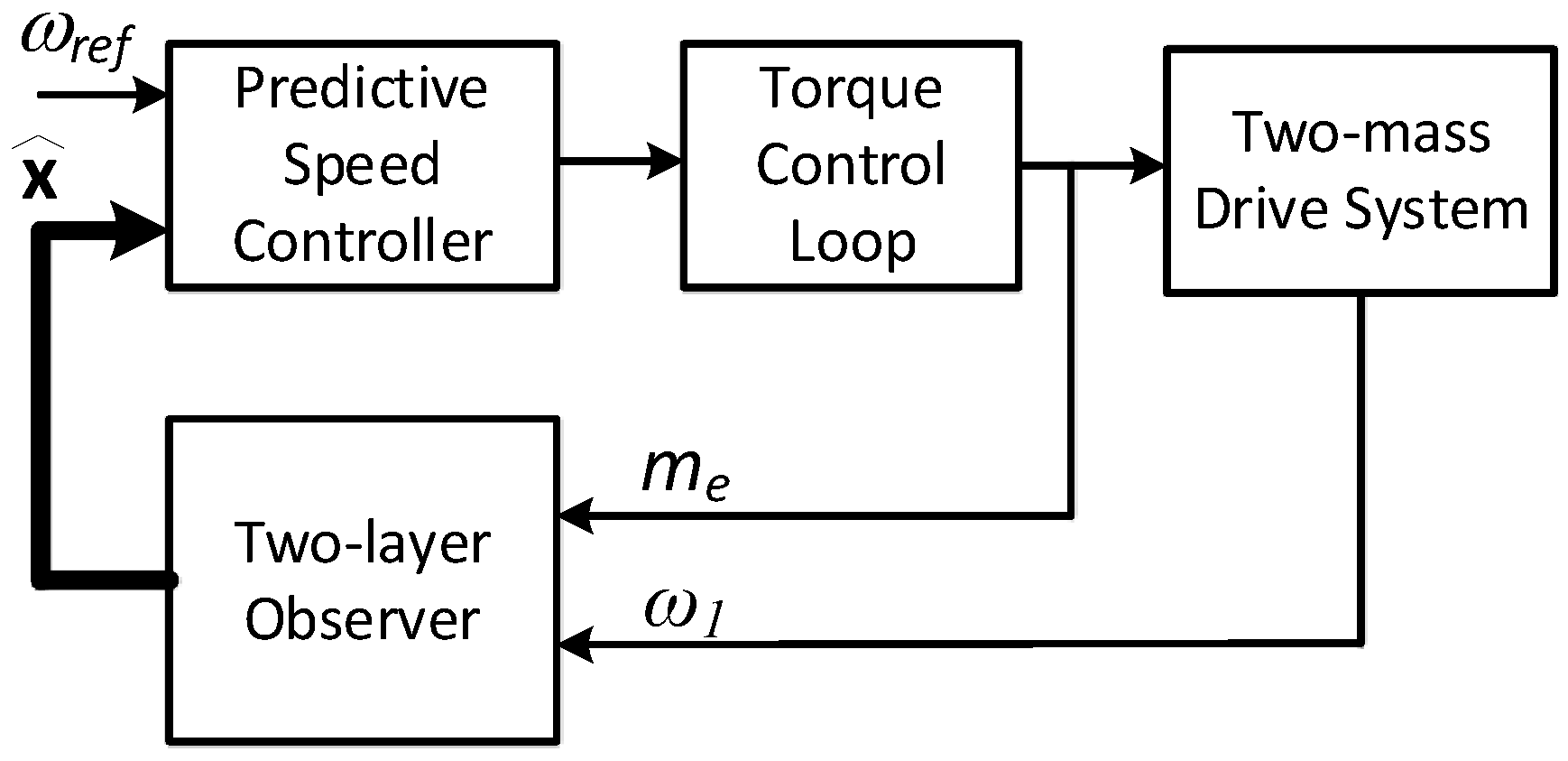
In cases where measurement of the state is difficult or impossible, estimation methods are used. This paper presents the predictive speed controller of the two-mass system cooperating with the classical Luenberger observer and with the two-layer version. The diagram of such a control structure is shown in Figure 2.

4. Luenberger Observer for the Two-Mass System

For a linear dynamic system, it is described by linear state equations (Equation (10a,b)) [22]:

$${\displaystyle \frac{d}{dt}}\mathbf{x}\left(t\right)=\mathbf{A}\mathbf{x}\left(t\right)+\mathbf{B}\mathbf{u}\left(t\right)$$

(10a)

$$\mathbf{y}\left(t\right)=\mathbf{C}\mathbf{x}\left(t\right)$$

(10b)

The Luenberger observer is defined by Equation (11a,b):

$${\displaystyle \frac{d}{dt}}\widehat{\mathbf{x}}\left(t\right)=\mathbf{A}\widehat{\mathbf{x}}\left(t\right)+\mathbf{B}\mathbf{u}\left(t\right)+\mathbf{K}[\mathbf{y}\left(t\right)-\widehat{\mathbf{y}}\left(t\right)]$$

(11a)

$$\mathbf{y}\left(t\right)=\mathbf{C}\widehat{\mathbf{x}}\left(t\right)$$

(11b)

In order to improve the control quality, the state vector was extended in the discrete model used in the predictive controller and in the observer algorithm (Equation (12)):

$$\widehat{\mathbf{x}}={\left[\begin{array}{cccc}{\widehat{\omega }}_1& {\widehat{\omega }}_2& {\widehat{m}}_s& {\widehat{m}}_L\end{array}\right]}^T$$

(12)

As a result, the state, control, and output matrices take the following form (Equation (13)):

$$\mathbf{A}=\left[\begin{array}{cccc}0& 0& {\displaystyle \frac{-1}{T_1}}& 0\\ 0& 0& {\displaystyle \frac{1}{T_2\left(t\right)}}& {\displaystyle \frac{-1}{T_2\left(t\right)}}\\ {\displaystyle \frac{1}{T_c\left(t\right)}}& {\displaystyle \frac{-1}{T_c\left(t\right)}}& 0& 0\\ 0& 0& 0& 0\end{array}\right]\mathbf{B}=\left[\begin{array}{c}{\displaystyle \frac{1}{T_1}}\\ 0\\ 0\\ 0\end{array}\right]\mathbf{C}={\left[\begin{array}{c}1\\ 0\\ 0\\ 0\end{array}\right]}^T$$

(13)

The gain matrix of the observer has four elements (Equation (14)):

$$\mathit{K}=\left[\begin{array}{cccc}{\displaystyle \frac{q_1}{T_1}}& {\displaystyle \frac{q_3}{T_2}}& {\displaystyle \frac{q_2}{T_c}}& q_4\end{array}\right]$$

(14)

The gain matrix coefficient was determined using the pole placement method, which can be summed up with Equations (15)–(18):

$$q_{\mathbf{1}}=4ap{T}_1$$

(15)

$$q_{\mathbf{2}}={\displaystyle \frac{T_1}{T_2}}+1-T_1{T}_c\left(4a^2+2\right)p^2$$

(16)

$$q_{\mathbf{3}}=4ap{T}_1\left(T_c{T}_2{p}^2-1\right)$$

(17)

$$q_{\mathbf{4}}=-T_1{T}_2{T}_c{p}^4$$

(18)

where p—resonance frequency, and a—damping coefficient.

5. Two-Layer Observer

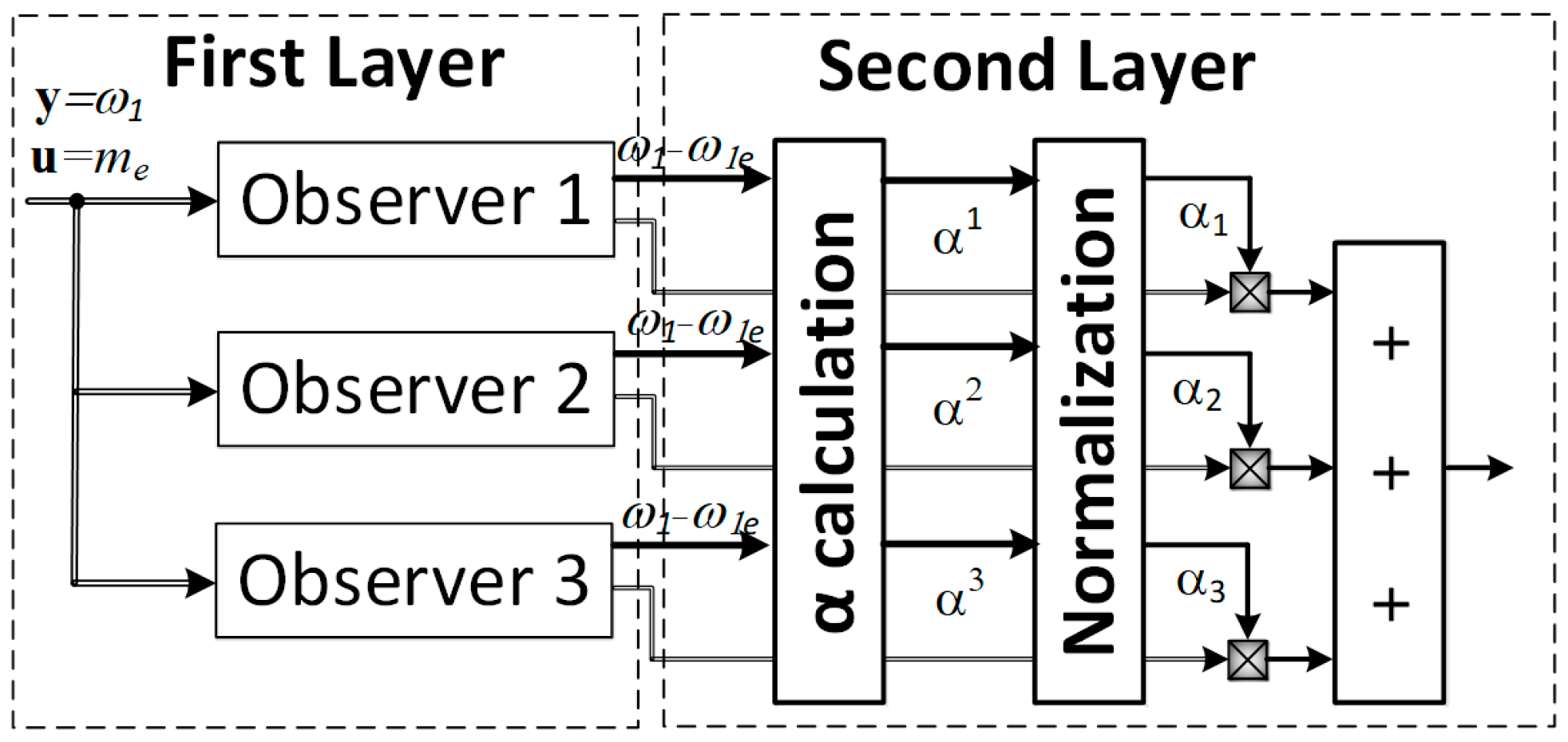
The structure of the two-layer observer consists of three independent Luenberger observer algorithms located in the first layer. Each of them works on the same signals, and they differ only in their initial state. In the second layer of the described estimator, the state vectors of each of the observers from the first layer are compared with each other and combined to produce a single common output state vector of the two-layer observer, as shown in Equation (19) [12,23,24,25] and Figure 3:

$$\mathit{x}={\alpha }_1{\mathit{x}}_1+{\alpha }_2{\mathit{x}}_2+{\alpha }_3{\mathit{x}}_3$$

(19)

where x—output state vector of the two-layer observer, x₁–x₃—output state vectors of the first-layer observers, and α₁–α₃—weight coefficients.

Equation (19) shows that the greater the weight coefficient of a given estimator from the first layer, the greater the influence of that estimator on the output signal of the two-layer estimator. Therefore, a higher coefficient should mean that the estimator from the first layer is closer to the real values. To compare observers, their estimation errors of drive speed ω₁ are used (the estimated values of each estimator from the first layer are compared with the real value), which form the basis for calculating the weighting factors α according to Equation (20) (appropriate formulas protect the algorithm against division by zero):

$${\alpha }^n={\left({\displaystyle \frac{1}{\gamma \int \left|{\omega }_{1m}-{\widehat{\omega }}_{1n}\right|dt-\beta {\Delta }_{\alpha }\left(t-1\right)}}\right)}^M$$

(20)

where γ—learning coefficient, M—power coefficient, ${\omega }_{1m}$—measured motor speed, ${\widehat{\omega }}_{1n}$—motor speed estimated by n-th estimator, β—forgetting factor, and Δ_α—sum of all errors within a certain sliding window of size defined by the parameter β.

The use of integration operations means that the formation of the values of the weighting coefficients is influenced by all obtained samples of estimation errors since the beginning of the algorithm. Therefore, a procedure for subtracting old samples multiplied by the forgetting factor β is introduced, limiting the influence of past signals. The block diagram of the two-layer Luenberger observer is presented in Figure 3.

The condition for obtaining the correct output state vector of the two-observer is to satisfy the relation (Equation (21)):

$${\alpha }_1+{\alpha }_2{+\alpha }_3=1$$

(21)

For this purpose, the values of the weighting coefficients α were normalised (Equation (22))—normalisation step in Figure 3:

$${\alpha }_n={\displaystyle \frac{{\alpha }^n}{{\sum }_{i=1}^n{\alpha }^i}}$$

(22)

It should be emphasised that the gains of the estimators in the first layer are selected using the pole placement method. This method ensures the arbitrary location of the poles of the closed system in the complex plane. This means that this method allows for shaping the dynamics of the observer and ensuring the stability of the estimators in the first layer. The mechanism used to combine signals from the first layer ensures the stability of the resulting two-layer estimator. The normalisation stage is particularly important here, as it causes the sum of the normalised weighting factors of all observers to equal one. Considering the above and the fact that the estimators from the first layer are stable, it can be concluded, in accordance with the principle of superposition, that the resulting observer is also stable.

6. Results

A series of simulation tests was carried out to compare the predictive control structure with the classic and two-layer observer. Simulation research was carried out in the MATLAB/Simulink (2010a) environment using a fixed step solver (ode1) with a step size of 500 μs. Three models of the two-mass drive system with a predictive controller were created. The models differed only in the source of the system state information; the first one used direct feedback from the plant, and it serves as an ideal, exemplary case; the second one used the classic Luenberger observer, and the third one used the two-layer version. The models were tested for three different state constraints for the torques: test 1—constraints for electromagnetic torque and torsional torque = ±3 p.u.; test 2—constraint for electromagnetic torque = ±3 p.u., and constraints for torsional torque = ±1.5 p.u.; test 3—constraints for electromagnetic torque and torsional torque = ±1.5 p.u. Before each test, the predictive controller was optimised for existing conditions, using an ideal model with direct feedback and a pattern search algorithm. The cost function described in Equation (23a,b) was used:

$$J=\sum \left|{\omega }_{ref}-{\omega }_1\right|\ast \sum \left|{\omega }_{ref}-{\omega }_2\right|+K$$

(23a)

$$where:K=\left\{\begin{array}{c}0\to fo\mathrm{r} m_s\le m_s^{max}\\ k(m_s-m_s^{max})\to for m_s>m_s^{max}\end{array}\right\}$$

(23b)

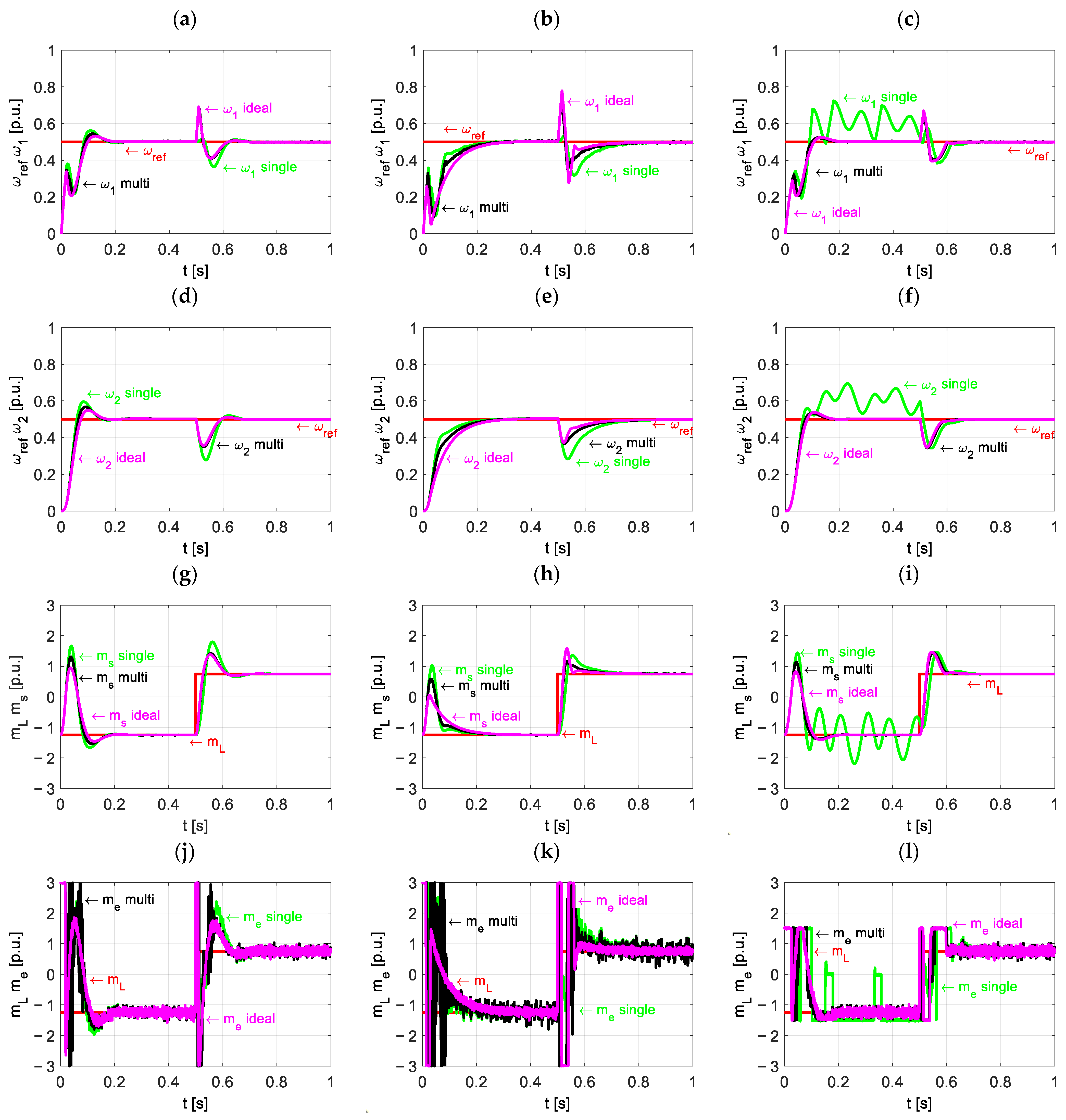
The parameters that remained the same in each test were as follows: prediction horizon N = 3, control horizon N_c = 2, state constraints for speeds = ±1.5, dynamic parameters for observers: a = 0.7, p = 120, initial state vector of the two-mass system [0 0 −1.25 −1.25], classic observer initial state vector—[0 0 0 0], and initial state vectors of the two-layer observer [0 0 −3 −3], [0 0 0 0], [0 0 3 3]. The controller was tested in an explicit version. The results of all three tests are shown in Figure 4.

In test 1 (Figure 4a,d,g,j), all three systems keep torque constraints; it is evident that the state variable transients of the system with the two-layer observer are closer to the transients of the ideal system than to the transients of the system with the classic observer. In test 2 (Figure 4b,e,h,k), all three systems still maintain more demanding torsional torque constraints, but this caused negative changes in speed transients, especially for the system with the classic observer. In test 3 (Figure 4c,f,i,l), the system with a classic observer keeps the torsional torque constraints, but significant oscillations occurred in its transients of the state variables, while the control quality of the system with a two-layer observer is still close to the ideal system with direct feedback. These observations are confirmed in

Table 1. Simulation results, differences between reference variables and real variables, and system comparison.

		Single Δ [-]	Two-Layer Δ [-]	Ideal Δ [-]	Single Δ [%]	Two-Layer Δ [%]	Ideal Δ [%]
Test 1	ω1	2.89 × 10−2	2.92 × 10−2	3.01 × 10−2	96.1	97.1	100
	ω2	3.78 × 10−2	3.26 × 10−2	3.24 × 10−2	116.7	100.6	100
	ms	2.44 × 10−1	1.98 × 10−1	1.87 × 10−1	130.4	105.8	100
	me	4.34 × 10−1	4.40 × 10−1	4.11 × 10−1	105.5	107.0	100
		Single Δ [-]	Two-Layer Δ [-]	Ideal Δ [-]	Single Δ [%]	Two-Layer Δ [%]	Ideal Δ [%]
Test 2	ω1	4.44 × 10−2	4.61 × 10−2	5.18 × 10−2	85.7	88.9	100
	ω2	4.86 × 10−2	4.45 × 10−2	4.83 × 10−2	100.7	92.1	100
	ms	1.91 × 10−1	1.57 × 10−1	1.54 × 10−1	123.9	101.8	100
	me	4.47 × 10−1	5.28 × 10−1	4.65 × 10−1	96.1	113.3	100
		Single Δ [-]	Two-Layer Δ [-]	Ideal Δ [-]	Single Δ [%]	Two-Layer Δ [%]	Ideal Δ [%]
Test 3	ω1	7.45 × 10−2	3.19 × 10−2	3.31 × 10−2	225.1	96.2	100
	ω2	7.52 × 10−2	3.30 × 10−2	3.37 × 10−2	222.9	97.9	100
	ms	3.84 × 10−1	1.80 × 10−1	1.80 × 10−1	213.6	100.2	100
	me	5.46 × 10−1	3.90 × 10−1	3.85 × 10−1	141.7	101.2	100

, which shows the sums of differences between reference variables (${\omega }_{ref}$, $m_L$) and each system’s real variables related to the number of samples (also known as mean absolute error) for each test according to Equation (24):

$$∆={\displaystyle \frac{\sum _{i=1}^N\left|v_{ref}-v\right|}{N}}$$

(24)

where $N$—total number of samples, $v_{ref}$—reference variable, and $v$—real variable.

Table 1 also shows the results of the system with a single observer and the system with the two-layer observer compared to the ideal system by Equation (25):

$$\delta ={\displaystyle \frac{{\Delta }_{single|multi}}{{\Delta }_{ideal}}}\times 100\%$$

(25)

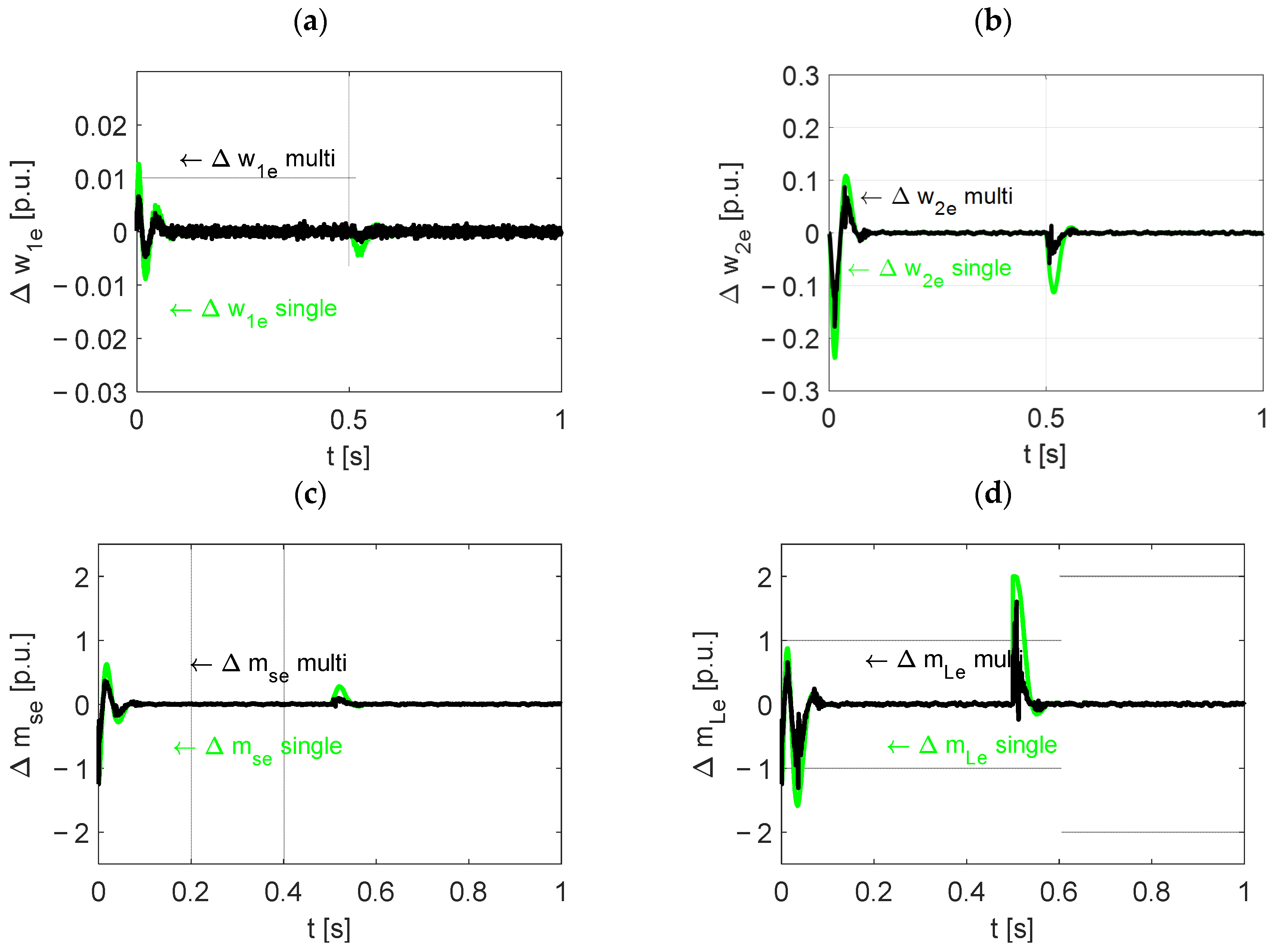
The advantage of a control system with a two-layer observer comes from the better quality of the estimated state variables, which is visible in Figure 5. This Figure shows transients of the estimation errors of the state variables from test 1, which proves that the two-layer observer estimation errors are smaller and run to zero faster. Better estimation ensures better predictions, which allows the regulator to better select the control track. In test 3, the levels of the estimation errors for both observers (two-layer and ideal) are the same as in test 1, but the torque limitations are lowered, and the level of errors generated by the classic observer makes it impossible to properly control the system’s work in such conditions.

The sum of errors related to the number of samples (mean absolute error) for the entire simulation is presented in

Table 2. Simulation test 1—Comparison of estimation errors: single classic observer and two-layer observer.

	Single Δ [-]	Two-Layer Δ [-]	Single Δ [%]	Two-Layer Δ [%]
ω1	7.24 × 10−4	5.13 × 10−4	141.1	100
ω2	9.9 × 10−3	4.70 × 10−3	212.1	100
ms	3.21 × 10−2	1.67 × 10−2	192.2	100
mL	1.11 × 10−1	0.48 × 10−1	231.6	100

according to Equation (26):

$$∆={\displaystyle \frac{\sum _{i=1}^N\left|v-v_e\right|}{N}}$$

(26)

where $N$—total number of samples, $v$—real variable, and v_e—estimated variable.

Table 2 also shows the results of both estimators compared by Equation (27):

$$\delta ={\displaystyle \frac{{\Delta }_{single}}{{\Delta }_{multi}}}\times 100\%$$

(27)

The experimental research was carried out on the test stand composed of two DC machines, motor and generator (their parameters are presented in

Table 3. Characteristics of the DC Motors.

	DC Motor	DC Generator
Manufacturer	INiME KOMEL (Sosnowiec, Poland)	INiME KOMEL (Sosnowiec, Poland)
Type	PZBB 22b	PZBB 22b
Power	500 W	400 W
Nominal voltage	220 V	230 V
Nominal armature current	3.15 A	3.15 A
Nominal excitation current	0.254 A	0.254 A
Nominal speed	1450 rpm	1450 rpm
Rotor resistance	8.05 Ω	8.05 Ω
Rotor inductance	0.8 H	0.8 H
Moment of inertia	0.0044 kgm2	0.0044 kgm2
Auxiliary poles resistance	2 Ω	2 Ω

), connected by a flexible shaft (600 mm long, made of steel 37HS), shown in Figure 6, for which the time constants of the components were determined to be 0.203 s for the motor, 0.203 s for the generator, and 0.0026 s for the shaft. The driving motor is powered by an H-bridge. The generator stator circuit is connected to the resistor via a single transistor. Both motors are connected with incremental encoders with a resolution of 36,000 pulses. LEM transducers are used as current sensors. The set also includes a dSPACE DS1103 (Paderborn, Germany) rapid prototyping board. Experimental control and monitoring were handled via the dSPACE Control Desk (Paderborn, Germany), while the hardware software was generated from the MATLAB/Simulink 2010a model using Coder.

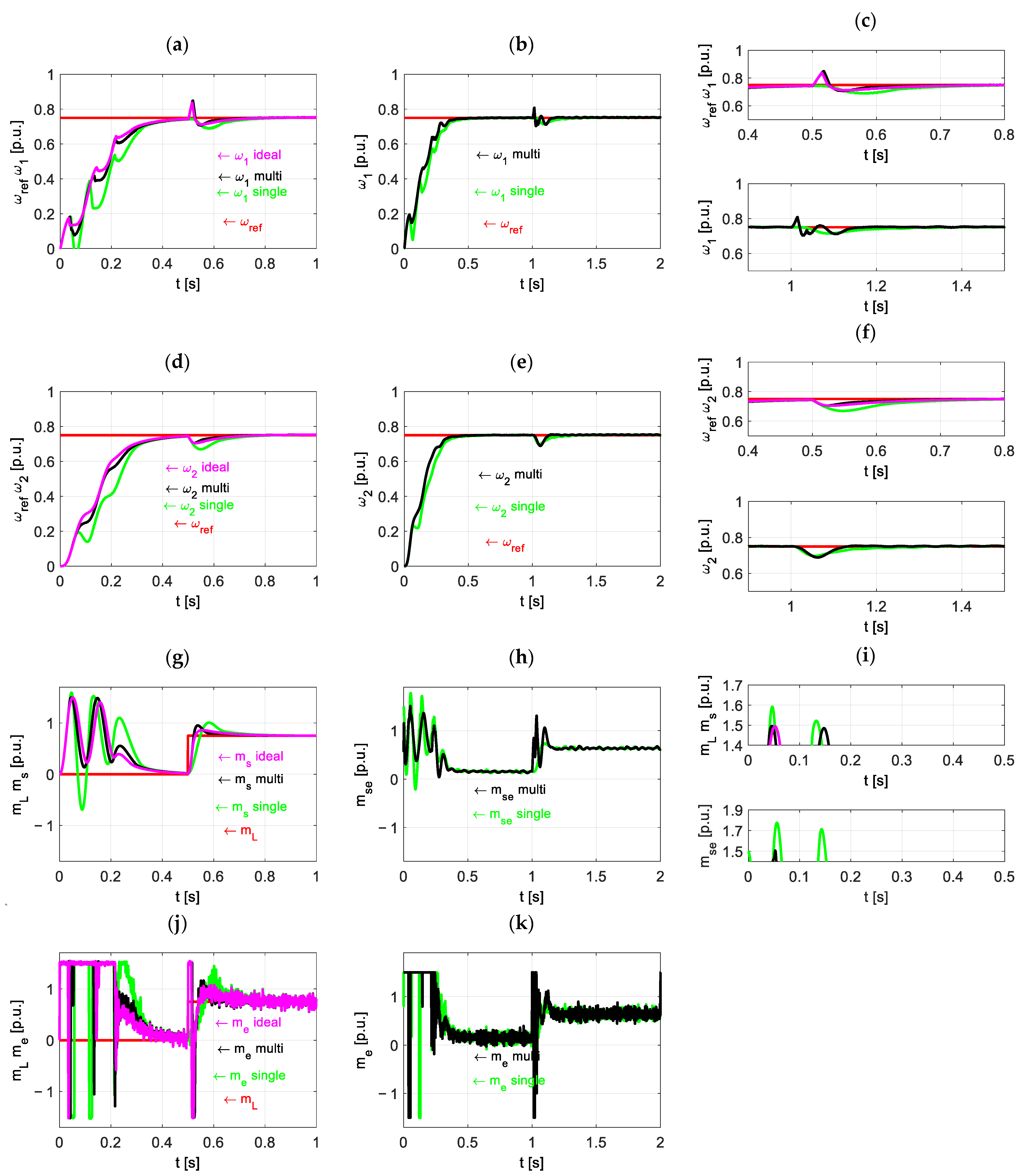
Another simulation test was designed that could be repeated experimentally on a test stand. Due to the fact that there was no possibility of setting the initial state other than zero, the situation was reversed and the following initial states in both observers were set: classic observer—[0 0 1.5 1.5], two-layer observer—[0 0 −1.5 −1.5], [0 0 1.5 1.5], [0 0 2 2], and in addition, the following parameters were changed: prediction horizon N = 10, control horizon N_c = 2, and dynamic parameters for observers: a = 0.7, p = 75. The simulation and experimental results are shown in Figure 7.

In both tests, it is evident that the predictive controller achieves better results with the two-layer observer than with the classic observer. This is especially noticeable during drive acceleration. The rise time for a two-layer system is approximately 0.1 s shorter. There is no overshoot in either system. In transients of the control system with the two-layer algorithm, it can also be observed that the speeds oscillate slightly (Figure 7a,b,d,e) and the estimated torsional torque does not exceed the set limits (Figure 7g,h,j,k). However, in transients of the control system with the classic observer, significant drive speed oscillations are visible (Figure 7a,b), which are partially transmitted to the load speed (Figure 7d,e). Furthermore, a predictive controller with a standard algorithm cannot maintain the set torsional torque limit (Figure 7g,h,j,k), especially in the experimental test (Figure 7i), where the torsional torque exceeds the value of 1.75 [p.u.], with a limit of 1.5 [p.u.]. Application of the two-layer observer also ensures faster disruption response—change in the load torque, although the difference is more visible in the simulation test (Figure 7f), but in the case of the experiment, the speed-settling time is at least 0.05 s shorter.

7. Conclusions

The conducted research allows the following conclusions to be drawn:

-

To reach its full potential, predictive control needs a high-quality reproduction of state variables by algorithms if it is impossible to measure them.

-

Significant improvements in estimation dynamics, especially in cases of unknown initial state of the control object, can be achieved with the help of a two-layer observer. In the simulation studies conducted, the system with a regulator and two-layer observer obtained similar results to the model with a regulator and direct feedback from the plant.

-

The use of a predictive controller with a two-observer for a two-mass drive system allows the imposition of stricter torsional torque limits while maintaining a better control quality than when using a classic observer. This is possible thanks to better estimation quality.

References

1. Chinoracky, R.; Stalmasekova, N.; Corejova, T. Trends in the Field of Electromobility—From the Perspective of Market Characteristics and Value-Added Services: Literature Review. Energies 2022, 15, 6144. [Google Scholar] [CrossRef]
2. Adamczyk, J.; Dzikuć, M.; Dylewski, R.; Varese, E. Assessment of selected environmental and economic factors for the development of electro-mobility in Poland. Transportation 2024, 51, 2199–2223. [Google Scholar] [CrossRef]
3. Kaczmarczyk, G.; Stanislawski, R.; Szrek, J.; Kaminski, M. Adaptive Sliding Mode Control Based on a Radial Neural Model Applied for an Electric Drive with an Elastic Shaft. Energies 2024, 17, 833. [Google Scholar] [CrossRef]
4. Żychlewicz, M.; Kamiński, M. The LSTM Models with Gated Recurrent Unit Applied for Shaft Torque Estimation of Two-Mass System. In Proceedings of the 2025 29th International Conference on Methods and Models in Automation and Robotics (MMAR), Miedzyzdroje, Poland, 26–29 August 2025; pp. 295–300. [Google Scholar] [CrossRef]
5. Derugo, P. Transfer Learning for Fuzzy Control of Two-Mass Drive System Using State Variables Feedback. In Proceedings of the 2023 10th International Conference on Electrical, Electronic and Computing Engineering (IcETRAN), East Sarajevo, Bosnia and Herzegovina, 5–8 June 2023; pp. 1–6. [Google Scholar] [CrossRef]
6. Kahsay, A.H.; Derugo, P.; Szabat, K.; Katsura, S. Design of Disturbance Observer-Based Robust Speed Control Structure for Two-Mass Drive System with the Help of Birch Optimization Algorithm. Energies 2025, 18, 1914. [Google Scholar] [CrossRef]
7. Mohammed, A.M.; Al-Samarraie, S.A.; Jaber, A. Design of a robust controller for a gearbox connected two-mass system based on a hybrid model. FME Trans. 2022, 50, 79–89. [Google Scholar] [CrossRef]
8. Kaczmarczyk, G.; Malarczyk, M.; Stanisławski, R.; Kamiński, M. Auto-Identification of Two-Mass System Parameters with Reinforcement Learning. In Proceedings of the 2025 29th International Conference on Methods and Models in Automation and Robotics (MMAR), Miedzyzdroje, Poland, 26–29 August 2025; pp. 289–294. [Google Scholar] [CrossRef]
9. Gorla, A.; Serkies, P. Comparative Study of Analytical Model Predictive Control and State Feedback Control for Active Vibration Suppression of Two-Mass Drive. Actuators 2025, 14, 254. [Google Scholar] [CrossRef]
10. Szabat, K.; Pajchrowski, T.; Tarczewski, T. Modern Electrical Drives: Trends, Problems, and Challenges. Energies 2022, 15, 160. [Google Scholar] [CrossRef]
11. Kaminski, M.; Tarczewski, T. Neural Network Applications in Electrical Drives—Trends in Control, Estimation, Diagnostics, and Construction. Energies 2023, 16, 4441. [Google Scholar] [CrossRef]
12. Niu, F.; Chao, X.; Zhang, Y.; Chen, J.; Li, S. MEKF-Tuned Full-State Feedback for Two-Mass Resonance Suppression. In Proceedings of the 2025 IEEE 12th International Symposium on Sensorless Control for Electrical Drives (SLED), Harbin, China, 15–17 August 2025; pp. 1–7. [Google Scholar] [CrossRef]
13. Vukojičić, S.; Ristić, L.; Kvaščev, G. Industrial application of neural network-optimized model predictive control for a two mass resonant mechanical system. Electr. Eng. 2025, 107, 14121–14136. [Google Scholar] [CrossRef]
14. Derugo, P.; Szabat, K. Adaptive neuro-fuzzy PID controller for nonlinear drive system. COMPEL Int. J. Comput. Math. Electr. Electron. Eng. 2015, 34, 792–807. [Google Scholar] [CrossRef]
15. Dodds, S.J.; Szabat, K. Forced Dynamic Control of Electric Drives with Vibration Modes in the Mechanical Load. In Proceedings of the IEEE 2006 12th International Power Electronics and Motion Control Conference, Portoroz, Slovenia, 30 August–1 September 2006; pp. 1245–1250. [Google Scholar] [CrossRef]
16. Jastrzębski, M.; Kabziński, J. Adaptive Control of Two-Mass System with Nonlinear Stiffness and Backlash. In Proceedings of the 2025 29th International Conference on Methods and Models in Automation and Robotics (MMAR), Miedzyzdroje, Poland, 26–29 August 2025; pp. 327–332. [Google Scholar] [CrossRef]
17. Wang, T.; Song, J. Research on Oscillation Suppression of Asymmetric Hydraulic Cylinder Flexible Connection Based on Luenberger Observer. In Proceedings of the 2022 3rd International Conference on Control, Robotics and Intelligent System, Virtual Event, 26–28 August 2022. [Google Scholar]
18. Huang, Y.; Zhang, Z.; Huang, W.; Chen, S. DC-Link Voltage Regulation for Wind Power System by Complementary Sliding Mode Control. IEEE Access 2019, 7, 22773–22780. [Google Scholar] [CrossRef]
19. Mayne, D.Q.; Rawlings, J.B.; Rao, C.V.; Scokaert, P.O. Constrained model predictive control: Stability and optimality. Automatica 2000, 36, 789–814. [Google Scholar] [CrossRef]
20. Raimondo, D.M.; Limon, D.; Lazar, M.; Magni, L.; Camacho, E.F. Min-max model predictive control of nonlinear systems: A unifying overview on stability. Eur. J. Control. 2009, 15, 5–21. [Google Scholar] [CrossRef]
21. Oyuela-Ocampo, J.-C.; Garcés-Ruiz, A.; Sanchez-Acevedo, S.; Ljøkelsøy, K.; D’Arco, S. Continuous Control-Set Model-Predictive Control with stability guarantee for the PWM-VSC. Control. Eng. Pract. 2025, 157, 106246. [Google Scholar] [CrossRef]
22. Szabat, K.; Tran-Van, T.; Kamiński, M. A modified fuzzy luenberger observer for a two-mass drive system. IEEE Trans. Ind. Inform. 2015, 11, 531–539. [Google Scholar] [CrossRef]
23. Śleszycki, K.; Wróbel, K.; Szabat, K.; Katsura, S. Parameter Identification of the Two-Mass System with the help of Multi-layer Estimator. In Proceedings of the 2021 IEEE 30th International Symposium on Industrial Electronics (ISIE), Kyoto, Japan, 20–23 June 2021. [Google Scholar] [CrossRef]
24. Szabat, K.; Tokarczyk, A.; Wróbel, K.; Katsura, S. Application of the Multi-Layer Observer for a Two-Mass Drive System. In Proceedings of the 2020 IEEE 29th International Symposium on Industrial Electronics (ISIE), Delft, The Netherlands, 17–19 June 2020; pp. 265–270. [Google Scholar] [CrossRef]
25. Szabat, K.; Wróbel, K.; Śleszycki, K.; Katsura, S. States Estimation of the Two-Mass Drive System Using Multilayer Observer. In Proceedings of the 2021 IEEE 19th International Power Electronics and Motion Control Conference (PEMC), Gliwice, Poland, 25–29 April 2021; pp. 743–748. [Google Scholar] [CrossRef]
Figure 1. Diagram of the two-mass system.
Energies 18 06113 g001
Figure 2. Block diagram of the considered control system.
Energies 18 06113 g002
Figure 3. Block diagram of a two-layer Luenberger observer.
Energies 18 06113 g003
Figure 4. Simulation results. Left column (a,d,g,j)—test 1, middle column (b,e,h,k)—test 2, and right column (c,f,i,l)—test 3.
Energies 18 06113 g004
Figure 5. Simulation results and estimation errors (ad).
Energies 18 06113 g005
Figure 6. Picture of the experimental test stand.
Energies 18 06113 g006
Figure 7. Simulation and experimental results: Left column (a,d,g,j)—simulation results, middle column (b,e,h,k)—experimental results, and right column (c,f,i)—close-up of details.
Energies 18 06113 g007