Article

Short-Term Load Forecasting for Electricity Spot Markets Across Different Seasons Based on a Hybrid VMD-LSTM-Random Forest Model

1
China Energy Zhejiang Energy Sales Co., Ltd., Hangzhou 310012, China
2
College of Energy and Mechanical Engineering, Shanghai University of Electric Power, Shanghai 200090, China
3
Sales Branch, State Grid Zhejiang Integrated Energy Service Company, Hangzhou 311500, China
*
Author to whom correspondence should be addressed.
Energies 2025, 18(23), 6097; https://doi.org/10.3390/en18236097
Submission received: 29 October 2025 / Revised: 11 November 2025 / Accepted: 18 November 2025 / Published: 21 November 2025

Abstract

Short-term load forecasting (STLF) is a core technical support for ensuring the safe and economic operation of power systems and efficient trading in electricity spot markets. To address the limitations of traditional forecasting models in handling the strong nonlinear and non-stationary characteristics of load data under electricity spot market conditions—where load is influenced by the coupling of multiple factors, such as meteorological conditions, electricity price signals, and seasonal patterns—we propose a hybrid forecasting model (VMD-PSO-LSTM-RF) that integrates Variational Mode Decomposition (VMD), Long Short-Term Memory (LSTM), Random Forest (RF), and Particle Swarm Optimization (PSO) to enhance the forecasting accuracy and market adaptability. First, VMD is applied to adaptively decompose the half-hourly power load data of a comprehensive user in Ningbo, Zhejiang Province, from July 2024 to June 2025. The original load series was decomposed into three components, effectively avoiding the mode aliasing problem common in traditional decomposition methods and providing high-quality inputs for subsequent forecasting. Simultaneously, meteorological data and temporal features were incorporated to construct a multi-dimensional input feature set, meeting the requirements of electricity spot markets for considering multiple influencing factors. Second, the PSO algorithm was used to optimize the key hyperparameters of LSTM and RF with seasonal differentiation. With the optimization, we aimed to maximize the Coefficient of Determination (R2) on the validation set, ensuring that the model parameters precisely matched the load fluctuation characteristics of each season. Finally, based on the feature differences of various frequency components, LSTM and RF were used to construct sub-models, and the final load value was obtained through weighted integration of the prediction results of each component. The results fully demonstrate that the proposed model can accurately capture the multi-scale fluctuation characteristics of load in electricity spot market environments, with forecasting performance superior to traditional single models and basic hybrid models; furthermore, the proposed model achieves precise extraction of multi-scale load features and in-depth temporal pattern mining, providing reliable technical support for efficient electricity spot market operation, as well as empirical references for formulating scenario-specific forecasting strategies and managing trading risks in electricity markets.

1. Introduction

Short-Term Load Forecasting (STLF) serves as a core technological support for the transition of power systems from traditional dispatch modes to market-oriented operations; its accuracy directly determines the efficiency of electricity market trading, the security of grid operation, and the economy of energy allocation. In the electricity spot market environment, the generation side relies on load forecasting to formulate unit commitment plans and spot bidding strategies, thereby avoiding issues such as redundant reserve capacity or surging peak-shaving costs caused by forecasting deviations. The grid side depends on load forecasting to optimize transmission corridor utilization rates, thereby reducing congestion risks and network losses. Meanwhile, the user side utilizes accurate load forecasting to participate in demand response programs, thereby achieving electricity cost savings by leveraging peak–valley price differences.
With the advancement of the “Dual Carbon” goals, the penetration rate of renewable energy continues to increase, but the intermittency of wind and photovoltaic power further exacerbates load fluctuations. Simultaneously, the coordinated operation of the electricity spot market and ancillary service markets results in a load that is influenced by multiple factors such as electricity price signals, energy storage charging/discharging behaviors, and demand response. Traditional forecasting methods, based on experience or single models, can no longer meet the market’s high requirements for forecasting accuracy and timeliness. There is an urgent need to construct high-precision forecasting models adapted to complex market environments.
As core indicators reflecting socio-economic activities and energy consumption characteristics, the changing patterns of power load are dynamically influenced by multiple factors, exhibiting significant nonlinear, non-stationary, and multi-scale characteristics. From the perspective of external influencing factors, meteorological conditions are the primary driving factors: high summer temperatures lead to sharp increases in cooling load; low winter temperatures drive up heating demand; and although loads are relatively stable during mild spring and autumn seasons, short-term weather events, such as rainfall or strong winds, can still cause load fluctuations. Temporal features are equally critical, as differences in electricity consumption patterns between weekdays and holidays, combined with the daily load fluctuations during peak and valley periods, form the periodic basis of load variation.
In the context of the electricity spot market scenario, the complexity of load forecasting is further elevated. On the one hand, real-time fluctuations in spot electricity prices guide users to adjust their electricity consumption behaviors (e.g., reducing non-essential load during high-price periods), creating a bidirectional feedback mechanism between load and electricity prices; on the other hand, the widespread integration of distributed generation and microgrids increases the uncertainty of load forecasting. The superposition of these factors causes power load sequences to exhibit multi-scale characteristics of “long-term trend–medium-term periodicity–short-term fluctuation–random disturbance”, posing severe challenges to short-term load forecasting.

1.1. A Review of Artificial Intelligence and Machine Learning Methods Research

Traditional load forecasting methods primarily include statistical models such as Multiple Linear Regression, Exponential Smoothing, Kalman Filtering, and Autoregressive Integrated Moving Average (ARIMA) [1]; these methods are simple to model and computationally fast, but they require high data stationarity and struggle to capture the nonlinear and non-stationary characteristics within load sequences. Consequently, their forecasting accuracy is limited when dealing with load fluctuations in complex market environments.
In recent years, artificial intelligence and machine learning methods have been widely applied in load forecasting. Support Vector Regression (SVR), Artificial Neural Networks (ANNs) [2], and deep learning models [3] can effectively capture nonlinear patterns and long-term dependencies in load sequences. Long Short-Term Memory (LSTM) networks [4] mitigate the vanishing or exploding gradient problems of traditional recurrent neural networks through their gating mechanisms, demonstrating strong adaptability in time-series forecasting. The authors of [5] proposed a hybrid load forecasting model based on an Attention mechanism, CNNs, and BiLSTM, with the results indicating that it could improve the forecasting accuracy. The authors of [6] developed a combined power load forecasting system composed of decomposition–denoising, individual forecasting modules, an optimization module, and an evaluation module, effectively enhancing the accuracy and efficiency of load forecasting. Meanwhile, the authors of [7] proposed a short-term power load forecasting algorithm based on a stacking ensemble of Convolutional Neural Network–Bidirectional Long Short-Term Memory–Attention mechanism (CNN-BiLSTM-Attention) and extreme Gradient Boosting (XGBoost), which significantly improved the load forecasting accuracy. The authors of [8] proposed a deep learning framework based on Multi-Task Learning (MTL), Convolutional Neural Networks (CNNs), and Long Short-Term Memory (LSTM); compared with other models, it demonstrated higher performance The authors of [9] proposed an SSA-CNN-LSTM-ATT model that combined a CNN-LSTM model with Sparrow Search Algorithm (SSA) optimization and an Attention mechanism, which was capable of accurately predicting power load. Furthermore, Random Forest (RF) [10], as an ensemble learning method, manages high-dimensional features, mitigates overfitting, and exhibits strong robustness to outliers, making it suitable for integration with other models to further enhance forecasting performance [11].

1.2. A Review of Research on Combined Forecasting Methods

Despite their advantages, individual models often struggle to fully utilize the multi-scale characteristics present in load data, especially in electricity market environments, where load is influenced by multiple factors, such as meteorological conditions, economic activity, electricity price signals, and holiday effects, where it exhibits a clear superposition of multi-frequency components. To better extract these features, decomposition methods (Empirical Mode Decomposition (EMD), Ensemble Empirical Mode Decomposition (EEMD), Variational Mode Decomposition (VMD), etc.) have been introduced into the field of load forecasting [12]; among these, VMD can adaptively decompose the original load sequence into multiple Intrinsic Mode Functions (IMFs) with specific frequency characteristics, effectively avoiding the mode mixing problem and providing subsequent forecasting models with smoother, more regular input sequences. The authors of [13] proposed a VMD-SelfAttention-LSTM hybrid forecasting method that decomposed the load series into multiple IMFs through modal decomposition, used a Self-Attention mechanism module to improve the LSTM, and combined VMD with the enhanced LSTM for power load forecasting. Using ANN and VMD-LSTM methods as control groups, the researchers verified that the Mean Square Error of the VMD-SelfAttention-LSTM hybrid model was lower than that of the other methods. The authors of [14] employed Successive Variational Mode Decomposition (SVMD) to address the instability and nonlinearity problems present in electricity data during the decomposition process; through a comprehensive comparison with six other models, they achieved the highest prediction accuracy with their model. The authors of [15] proposed an ensemble learning model based on Long Short-Term Memory (LSTM), Variational Mode Decomposition (VMD), and a Multi-Strategy Optimized Dung Beetle Optimizer (MODBO), enhancing the global optimization capability. The authors of [16] proposed a short-term power load forecasting model (IZOA-VMD-TSK-TFS-TCA) based on a Takagi–Sugeno–Kang Transfer Fuzzy System (TSK-TFS) combined with Variational Mode Decomposition (VMD), Transfer Component Analysis (TCA), and an Improved Zebra Optimization Algorithm (IZOA). In this method, VMD was used to decompose the power load data into several subsequences, TCA was used for the dimensionality reduction in factors related to power load, and IZOA was employed to optimize the parameters of the TSK-TFS, using a subtractive clustering algorithm to obtain the number of clusters. Data from the source domain were then input into the TSK fuzzy system to obtain and retain the antecedent and consequent parameters. The experimental results show that the IZOA-VMD-TSK-TFS-TCA short-term power load forecasting model has high prediction accuracy.The core characteristics of existing short-term load forecasting models are summarized in Table 1 as follows:
For load forecasting, existing models exhibit distinct characteristics: LSTM, LSTM-GRU, Stacking-Fusion, and Reseamble-Model excel in time-series modeling with multi-model fusion robustness but suffer from hyperparameter sensitivity and high tuning costs; Shuffle-Transformer-Multi and Transformer-Attention-Net leverage self-attention for multi-variable interaction but face issues of high computational complexity and poor small-scene adaptability; CNN-LSTM, CNN-BiGRU, and ResNet-LSTM combine CNN’s spatial feature capture with LSTM/GRU’s temporal modeling but have complex structures and high preprocessing demands; Multi-task Learning and Source-Load Integrated Forecasting Model enable multi-scenario adaptability via collaborative learning but risk inter-task interference and complex design; Two-layer Joint Modal Decomposition Dynamic Ensemble Model, Stacking Ensemble, and Copula Correlation Analysis Fusion reduce sequence complexity through hierarchical decomposition and ensemble learning while incurring high training and computational costs.

1.3. Content and Contributions

Based on the above analysis, we propose a short-term load forecasting method combining VMD, LSTM, and RF to enhance prediction accuracy and robustness in electricity market environments. Specifically, VMD is first utilized to decompose the original load sequence into multiple subsequences, capturing different fluctuation characteristics of the load; then, for subsequences with different characteristics, LSTM and RF are employed to construct forecasting models, with model performance further improved through feature importance analysis and parameter optimization. Finally, the forecasting results of each subsequence are aggregated to obtain the final load forecast. The main contributions of this paper are as follows:
Multi-scale feature extraction: We utilize VMD to effectively decompose the load sequence, highlighting the characteristics of different frequency components and laying the foundation for subsequent forecasting.
Hybrid model forecasting: We combine the advantage of LSTM in modeling long-term dependencies in time series with the strengths of RF in handling high-dimensional features and robustness to build subsequence forecasting models.
Adaptability for electricity markets: We comprehensively consider market-related factors, such as meteorology and holidays, to improve the model’s forecasting capability and practicality in complex market environments.
Through a case study using actual electricity market load data, we verify the advantages of the proposed method regarding forecasting accuracy, stability, and computational efficiency, providing technical support for electricity market participants’ trading decisions and system operation.
The remainder of this paper is organized as follows. In Section 2, we describe the required algorithms and the proposed model. In Section 3, we introduce the load data, evaluation metrics, and parameter settings used in the experiments. In Section 4, we discuss the load forecasting results. In Section 5, we present the conclusions of this study.

2. Proposed Short-Term Load Forecasting Model

2.1. Fundamental Methods

2.1.1. Principle of VMD

Variational Mode Decomposition (VMD) is an adaptive signal decomposition method designed to decompose the original signal into a set of Intrinsic Mode Functions (IMFs) with specific frequency characteristics while effectively avoiding the mode mixing problem commonly encountered in traditional EMD methods.
VMD decomposes a signal into multiple bandwidth-limited modes by constructing and solving a constrained variational problem in which each mode oscillates around its central frequency; this method simultaneously considers the time- and frequency-domain characteristics of the signal during decomposition, enabling a more accurate extraction of features at different scales. The mathematical expression of the constrained variational model is as follows:
m i n U k , Ω k k = 1 K t δ t + j π t u k t e j ω k t 2 2 s . t . k = 1 K u k = f t
where U K   =   { u 1 , u 2 , . . . , u K } is each mode function; Ω K   =   { ω 1 , ω 2 , . . . , ω k } is each center frequency; δ t is the Dirac delta function; K is the number of decomposition layers; j is the imaginary unit; *   is the convolution operator; and f t is the original signal.
Introducing a penalty factor α and a Lagrangian multiplier operator λ , the constrained problem is transformed into the following unconstrained variational problem:
L { U κ } , { Ω κ } , λ = α k = 1 K α δ t + j π t * u k t e j ω λ t 2 2 + f t k = 1 K u k t 2 2 + λ t , f t k = 1 K u k t

2.1.2. LSTM Neural Network

Long Short-Term Memory (LSTM) [28] is a deep learning model that improves upon the Recurrent Neural Network (RNN); its core advantage lies in its special gating mechanism, which solves the problems of vanishing or exploding gradients that commonly occur in traditional RNNs when processing long sequence data, enabling LSTM to effectively capture long-term dependencies in time series, leading to its widespread application in forecasting tasks involving data with clear temporal characteristics, such as power load [29].
The core structure of LSTM [30] is the Memory Cell; its state update is collaboratively controlled by three key components: the Input, Forget, and Output Gates. Each component uses Sigmoid or tanh activation functions to screen and transmit information. A general LSTM structure is shown in Figure 1 [31].
The specific working mechanism is as follows:
(1) Forget Gate
The function of the Forget Gate is to decide whether to discard information from the Memory Cell of the previous time step; its inputs are the hidden state output from the previous time step h t 1   and the current time step’s input x t ; it uses a Sigmoid activation function to output a probability value between 0 and 1—a value closer to 1 means retaining the historical information, while a value closer to 0 means discarding it.
The mathematical expression is as follows:
f t = σ W f h t 1 , x t + b f
where   W f is the weight matrix of the Forget Gate, b f is the bias term, and   σ represents the Sigmoid activation function.
(2) Input Gate and Candidate Memory Cell
The Input Gate is responsible for screening the effective input information at the current time step; it also uses a Sigmoid activation function to output a probability value, determining the proportion of current information to retain. Simultaneously, combined with h t 1 and x t , it uses a tanh activation function to generate the Candidate Memory Cell C ^ t , which is used to update the state of the memory cell.
The mathematical expression is as follows:
i t = σ W i h t 1 , x t + b i C ^ t = t a n h W c h t 1 , x t + b c
where W i and W c are the weight matrices of the Input Gate and Candidate Memory Cell, respectively; b i and b c are the corresponding bias terms; and the tanh activation function maps the candidate information to the range [−1,1].
(3) Memory Cell State Update
The update of the Memory Cell state   C t combines the historical information filtered through the Forget Gate and the current candidate information filtered through the Input Gate, enabling the continuous transmission and updating of information across long sequences.
The mathematical expression is as follows:
C t = f t C t 1 + i t C ^ t
where C t 1   is the Memory Cell state from the previous time step.
(4) Output Gate and Hidden State Output
The Output Gate determines which information from the Memory Cell is passed to the hidden state output at the current time step: it first filters the Memory Cell information using a Sigmoid activation function, then multiplies the result with the Memory Cell state mapped with the tanh activation function to obtain the final hidden state output, which is used for the current prediction and serves as input for the next time step.
The mathematical expression is as follows:
o t = σ W o h t 1 , x t + b o h t = o t t a n h C t
where W o is the weight matrix of the Output Gate, and   b o is the bias term.

2.1.3. Random Forest Algorithm

Random Forest [32] is a machine learning algorithm, based on ensemble learning, that combines the prediction results of multiple decision tree models to perform classification or regression tasks. Due to its strong resistance to overfitting, adaptability to high-dimensional features, and straightforward parameter tuning process, it holds significant application value in complex time-series forecasting scenarios, such as power load prediction.
The core of Random Forest lies in its “randomness” and “ensemble” characteristics: through dual random sampling of both samples and features, multiple independent decision trees are generated; the results of these individual decision trees are then integrated through voting or averaging to reduce the variance of a single decision tree and enhance the overall generalization ability of the model. The specific implementation logic is as follows: the Bootstrap resampling method is used to randomly extract several sample subsets from the original training set, with each sample subset used to train an independent decision tree. At each split node of every decision tree, instead of using all features, a random subset of features is selected as candidate splitting features. The optimal split point is chosen based on indicators such as information gain or Gini coefficient to avoid excessive influence of any single feature on the model. For regression tasks, such as load forecasting, the final prediction result of the Random Forest is the arithmetic mean of the predicted values from all decision trees. Through the “collective decision making” of multiple decision trees, potential overfitting or prediction bias that may exist in a single decision tree is effectively offset.

2.1.4. Particle Swarm Optimization Algorithm

Particle Swarm Optimization (PSO) is a heuristic optimization method based on swarm intelligence; its design is inspired by the simulation of cooperative behaviors in biological groups, such as bird flocking for foraging or fish schooling for migration. The core idea involves searching for the efficient global optimum in the solution space through information interaction and dynamic adjustments between individuals (particles) within the group. Due to its intuitive principles, fast convergence speed, and strong adaptability to complex nonlinear optimization problems, this algorithm is widely applied in areas such as parameter tuning for machine learning models and feature selection; particularly, in hybrid model frameworks for power load forecasting, it is often used to optimize the key parameters of forecasting models or enhance the efficiency of feature selection, thereby improving the model’s fitting and predictive performance for load sequences.
The PSO algorithm abstracts each potential solution to an optimization problem as a “particle”, and all particles form a “particle swarm”, wherein each particle possesses two core attributes: position and velocity. Position corresponds to a potential solution in the solution space, while velocity determines the direction and step size of the particle’s movement in the solution space. The algorithm iteratively updates the velocity and position of the particles, enabling the particle swarm to gradually approach the optimal solution. The specific implementation mechanism is as follows:
If the dimensionality of the solution space for the optimization problem is D, and the size of the particle swarm is N, then the position of the i-th particle can be represented as X i = x i 1 , x i 2 , . . . , x i D , and its velocity can be represented as V i = v i 1 , v i 2 , . . . , v i D . During the iterative process, each particle records the best position it has found, known as the individual optimal solution P b e s t , i = p i 1 , p i 2 , . . . , p i D ; simultaneously, through information sharing, the particle swarm records the best position found within the entire group, known as the global optimal solution G b e s t = g 1 , g 2 , . . . , g D . The velocity and position of the particles are dynamically updated using the following formulas to ensure movement toward the optimal solution.
The velocity and position update formulas are as follows:
V i t + 1 = ω V i t + c 1 r 1 P b e s t , i t X i t + c 2 r 2 G b e s t t X i t
X i t + 1 = X i t + V i t + 1
where t is the current iteration number; ω is the inertia weight, used to balance the global exploration and local exploitation capabilities of the particle; c 1 and c 2 are learning factors, which adjust the weight of the particle moving toward its own optimal solution and the global optimal solution, respectively; and r 1 and r 2 are random numbers in the range [0,1], which can increase the randomness of the search process and prevent the algorithm from falling into local optima.

2.2. Proposed Forecasting Model

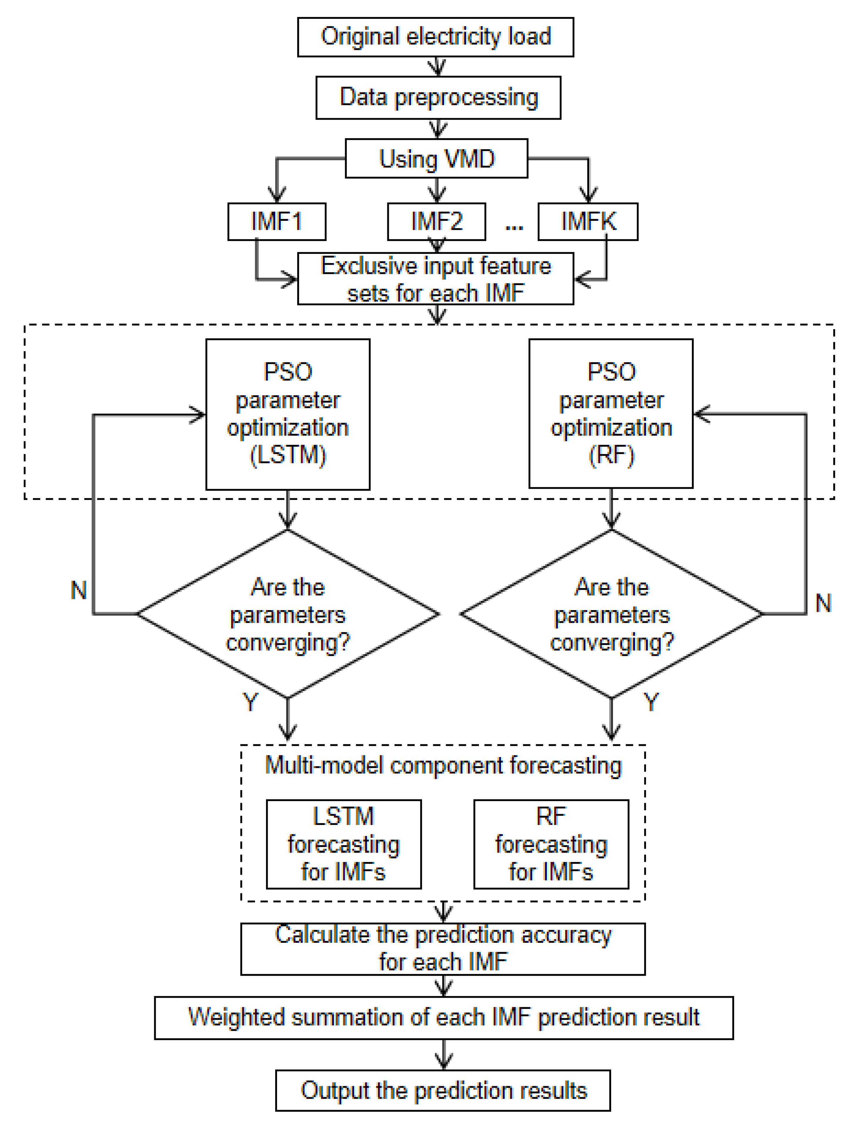
In this study, we propose a VMD-, LSTM-, RF-, and PSO-based STLF method with which to address the uncertainty and volatility in electricity spot markets. The workflow of the proposed model is illustrated in Figure 2, with each step described as follows:
The overall workflow of the power load forecasting method proposed in this paper follows a step-by-step logic of “data preprocessing-multi-scale decomposition–parameter optimization–multi-model prediction–weighted integration”. The specific steps are as follows:
Step 1: Raw power load and related influencing factor data were collected; after preprocessing the data by filling missing values and removing outliers, Variational Mode Decomposition (VMD) was applied to adaptively decompose the preprocessed original load sequence into K modal components with distinct frequency characteristics, achieving the separation of high-frequency random fluctuations, mid-frequency periodic features, and low-frequency trend features in the load.
Step 2: For each VMD-decomposed component, a dedicated input feature set was constructed based on the frequency characteristics of the component to reduce interference from redundant information.
Step 3: The PSO algorithm was introduced to optimize the key hyperparameters of LSTM and RF separately. Using hyperparameters, such as the hidden layer dimension, learning rate, and number of hidden units for LSTM, the number of decision trees and maximum tree depth for RF as optimization variables, and the R2 of the model validation set as the fitness function, the optimal parameter configurations were determined for both types of models through iterative updates of particle velocity and position in PSO.
Step 4: Based on the optimized parameters, the LSTM and RF prediction models were constructed, respectively. A dual-model collaborative modeling strategy was adopted for all VMD-decomposed components: utilizing the exclusive input feature set of each component, LSTM was used to capture the long-term and short-term temporal dependencies of each component, and RF was employed to explore the multi-dimensional correlation patterns between each component and factors such as meteorological and temporal features. This fully leverages the complementary advantages of the two types of models and avoids the fitting limitations of a single model for mixed-feature components.
Step 5: The forecasting accuracies of LSTM and RF were calculated for each component, and the weighting coefficients for each component were derived through normalization.
Step 6: A weighted summation of the LSTM and RF forecasting results was performed for each component using the determined weighting coefficients to obtain the final power load forecast value and output the prediction results.

2.3. Evaluation Metrics

To objectively and quantitatively validate the performance of the proposed VMD-PSO-LSTM-RF hybrid model in the half-hourly load forecasting task for a Ningbo user, we selected Root Mean Square Error (RMSE) and the Coefficient of Determination (R2) as the core evaluation metrics, as they complementarily measure the model’s forecasting effectiveness from the dimensions of “overall deviation degree” and “data fitting capability”, respectively, ensuring the rationality and comparability of the experimental results. Additionally, considering the requirements of load forecasting in the electricity spot market context, the practical significance of each metric is clarified below.
RMSE was used to quantify the overall deviation between the model’s predicted values and the actual load by calculating the square root of the mean of the squared differences between the predicted and actual values. The calculation formula is as follows:
R M S E = 1 N i = 1 N y i y ^ i 2
where N is the total number of forecast samples, y i is the actual load value at the i-th time point, and y ^ i is the model-predicted load value at the i-th time point.
R2 was used to measure the model’s ability to explain the variation in the actual load data by comparing the explanatory power of the model’s predicted values to that of the mean of the actual load; it is used to assess the degree to which the model fits the underlying patterns in the load data. The calculation formula is as follows:
R 2 = 1 i = 1 N y i y ^ i 2 i = 1 N y i y 2
where y is the sample mean of the actual load.

3. Case Study: Integrated Energy Sector

3.1. Data Source and Preprocessing

In the research of power load forecasting, the selection of data sampling granularity directly affects the forecasting accuracy and application value. Restricted by the actual data collection conditions, 15 min high-frequency data were not obtained in this study. For daily-level and 1-h-level sampling granularities, the literature analysis showed that 30-min-level sampling can not only capture the key fluctuations of intraday load peaks and valleys but also achieve a balance between data volume and computational efficiency. Its accuracy is superior to that of 1-h-level sampling [33] while avoiding the redundant computation and storage pressure associated with 15-min-level data.
In this study, we selected one year of power load data (from July 2024 to June 2025) from a user in the Ningbo area served by a power company in Zhejiang Province as the experimental sample. The data collection frequency was every half hour, resulting in a total of 17,520 valid records for the year. The daily average load is shown in Figure 3. As Ningbo is one of the core pilot areas for the Zhejiang electricity spot market, this user’s load includes both commercial complex and industrial production components; their electricity consumption behavior is not only influenced by seasonal variations, meteorological conditions, production schedules, and residential habits, but is also deeply correlated with price signals from the electricity spot market. For example, during peak spot price periods, industrial users adjust their production loads to reduce electricity costs, while commercial users exhibit lower sensitivity to electricity prices due to rigid loads such as air conditioning; this dual characteristic of “market orientation + rigid demand” causes the load sequence to exhibit more complex nonlinear and non-stationary characteristics, which is consistent with the multi-factor interference features of power load described in the literature and better aligns with the actual electricity consumption patterns of users in the electricity spot market, making it suitable for validating the practicality of the proposed model.
To comprehensively capture the factors influencing load, two types of data were simultaneously collected: first, meteorological data for the Ningbo area from July 2024 to June 2025, recorded at half-hour intervals daily, including temperature, humidity, wind speed, and total solar radiation; and second, temporal feature data, such as hour, day of the week, and holiday indicators. The various data formed a multi-dimensional input feature set of “load–meteorology–time”, meeting the core requirement of considering market signals for load forecasting in the electricity spot market.
In the data preprocessing stage, missing values caused by equipment failures were addressed using a collaborative linear interpolation method that incorporates both adjacent load values and electricity prices, an approach that differs from single-variable load interpolation by accounting for the guiding effect of spot market prices on load.
As can be seen from Figure 3, the load exhibited significant seasonal fluctuations, as follows:
The winter load remained at a relatively high level, with peaks approaching or exceeding 350 kWh, primarily due to the cold climate, in which extensive use of heating equipment significantly increased energy consumption, leading to higher load.
The summer load also stayed within a relatively high range. Although the overall peak was generally lower than in winter, it was noticeably higher than in spring and autumn. High temperatures in summer drive the widespread operation of cooling equipment, which is the main factor contributing to the increased load.
The spring and autumn loads were relatively lower, with the spring load being the lowest throughout the year. The mild climate during these two seasons greatly reduces the reliance on heating and cooling equipment, resulting in a corresponding decrease in energy consumption.
To enhance the model’s predictive performance, the load data was divided seasonally as follows: June, July, and August represent summer; September, October, and November represent autumn; December, January, and February represent winter; and March, April, and May represent spring. For each season, two sets of data were selected; the test sets included the week with the highest temperatures in summer and one randomly selected week, with the remaining data used as the training set. Similarly, for winter, the week with the lowest temperatures and one randomly selected week formed the test set, while the rest of the data served as the training set. For spring and autumn, two randomly chosen weeks were used as the test set, with the remaining data allocated to the training set.
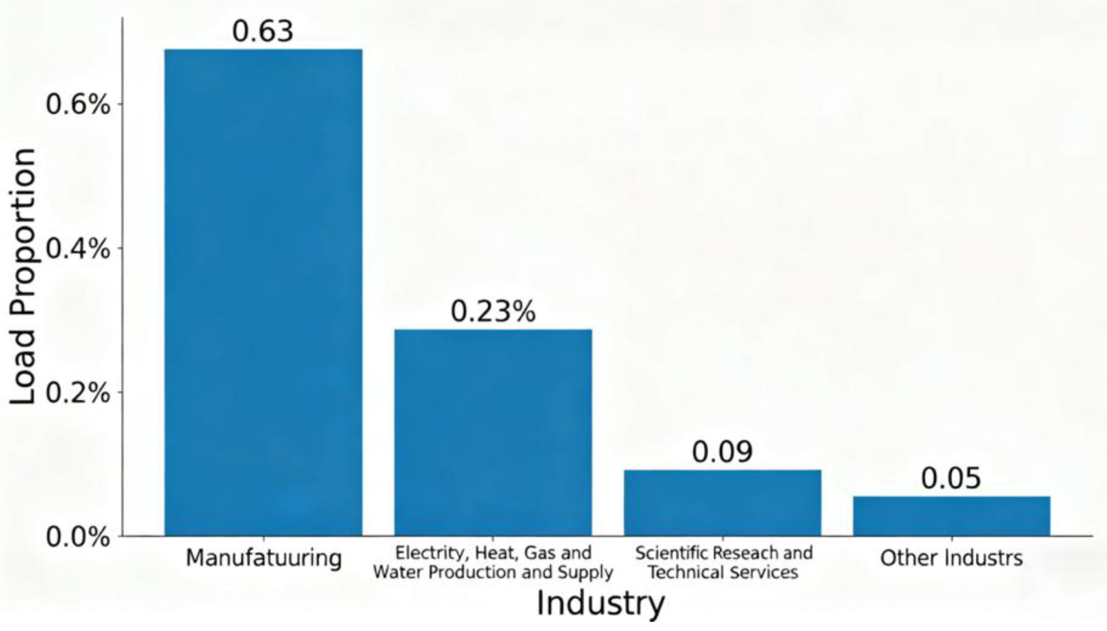
The research object of this paper was a group of comprehensive multi-industry users in the Ningbo area, covering 18 industries including wholesale and retail, manufacturing, scientific research, and technical services. The user load composition exhibited distinct characteristics of diversified industry coverage, core industry dominance, and differentiated load features. Among the core industries, manufacturing had the largest load scale, with stable intraday fluctuations and strong periodicity; the production and supply industry of electricity, heat, gas, and water was a secondary core industry, showing obvious seasonal fluctuations; the scientific research and technical services belonged to the medium-scale industry; the auxiliary industries covered 15 sub-fields such as wholesale and retail, and real estate. Overall, the load possessed core characteristics of industrial diversity, hierarchical differentiation, and temporal integrity, which not only ensures the representativeness of the research but also provides data complexity. This serves as an ideal data source for verifying the effectiveness of the integrated modeling approach combining VMD decomposition and LSTM-RF. The load proportion of different industries is shown in Figure 4.

3.2. Parameter Settings

To ensure the scientific rigor and adaptability of the model parameter configuration, we employed the Particle Swarm Optimization (PSO) algorithm to intelligently optimize the key hyperparameters of the Long Short-Term Memory (LSTM) network and Random Forest (RF) method, rather than relying on empirical settings. The specific parameter optimization logic and results are detailed below, ensuring the rationality and comparability of the experimental design.

3.2.1. VMD Parameter

As the core module for the multi-scale decomposition of load sequences, the parameters of VMD directly determine the completeness and regularity of the decomposed modal components. Parameter settings were divided into the following two categories: “basic fixed parameters” and “dynamic adaptable parameters”. Basic fixed parameters are empirical values ensuring decomposition stability, while dynamic adaptable parameters can be flexibly adjusted based on the characteristics of the load data. The specific settings and their functions are as follows:
Dynamic adaptable parameters: The core parameters were the number of decomposition modes K and the penalty factor α . The default value of K was set to 3. Through trial calculations, this value was verified to effectively separate the Ningbo user’s load into “high-frequency random fluctuations, mid-frequency intraday periodic patterns corresponding to peak–valley electricity consumption, and low-frequency trend components corresponding to seasonal electricity consumption characteristics”. This avoids the computational redundancy caused by an excessive number of modes or feature loss due to an insufficient number of modes. The default value of α was set to 2000.
The core parameters were the number of decomposition modes K and the penalty factor α . In VMD, the selection of the number of modes K needs to balance the integrity of load features and computational efficiency. Herein, the default value of K was set to 3, and this setting was mainly determined by referring to existing research results and verifying with data characteristics. When K = 3, the decomposition results corresponded exactly to three types of physical features (high-frequency, medium-frequency, and low-frequency components), therefore, K = 3 was finally determined [34].
Basic fixed parameters: Noise tolerance τ was fixed at 0; whether to enforce DC component decomposition DC was fixed at 0; the center frequency initialization method in it was fixed at 1; and the convergence threshold tol was fixed at 1 × 10⁻⁷.
The VMD parameterization is shown in Table 2.

3.2.2. PSO Parameter

The PSO algorithm was employed to intelligently optimize the key hyperparameters of LSTM and RF. The parameters were divided into two categories, “core PSO algorithm parameters” and “search ranges for model parameters to be optimized”, both designed based on the accuracy requirements and computational efficiency of the Ningbo user load forecasting task. First, the core parameters of the PSO algorithm were as follows: the number of particles was set to 20, the maximum number of iterations was set to 40, the inertia weight was set to 0.9, and the cognitive and social coefficients were set to 2.0. The search ranges for the model parameters to be optimized with PSO were as follows: In the LSTM model, the search range for the number of hidden layer neurons was set to [32,128], which balances model fitting capability and overfitting risk. The search range for the number of stacked layers was [1,2], avoiding gradient vanishing caused by excessive layers. The search range for the learning rate of the Adam optimizer was [0.0001,0.01], covering the commonly used learning rate range for deep learning models and avoiding training oscillations due to excessively high learning rates, or slow convergence due to excessively low learning rates. In the RF model, the search range for the number of decision trees was [10,50] to balance model stability and computational efficiency, avoiding increased computation time due to an excessive number of trees. The search range for the maximum depth of a single tree was [3,15], which limited the complexity of individual trees through depth control, reduced overfitting risk, and adapted to the processing requirements of high-dimensional “load-meteorology-time” features. The PSO parameter settings are shown in Table 3.

4. Results and Discussion

4.1. VMD Decomposition

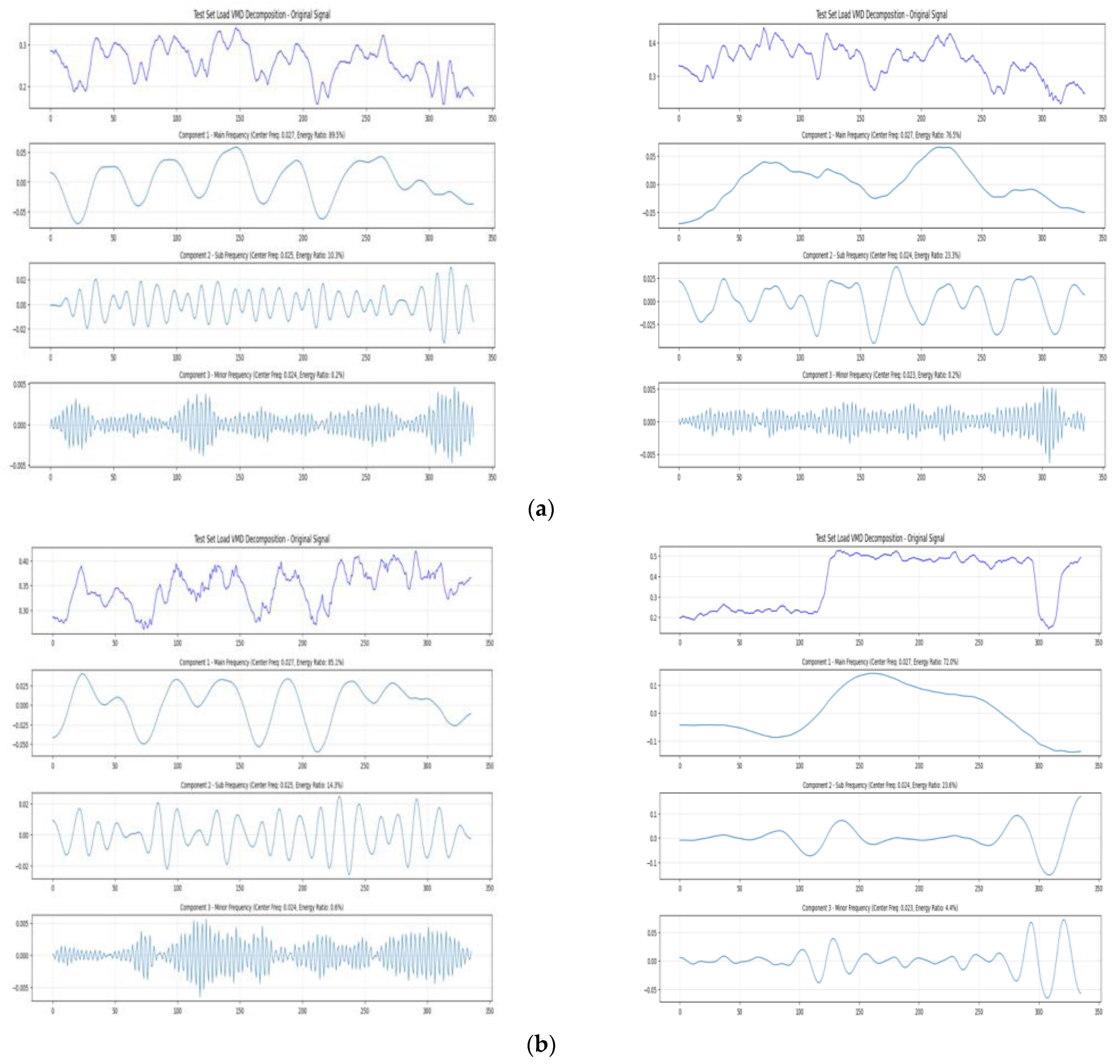
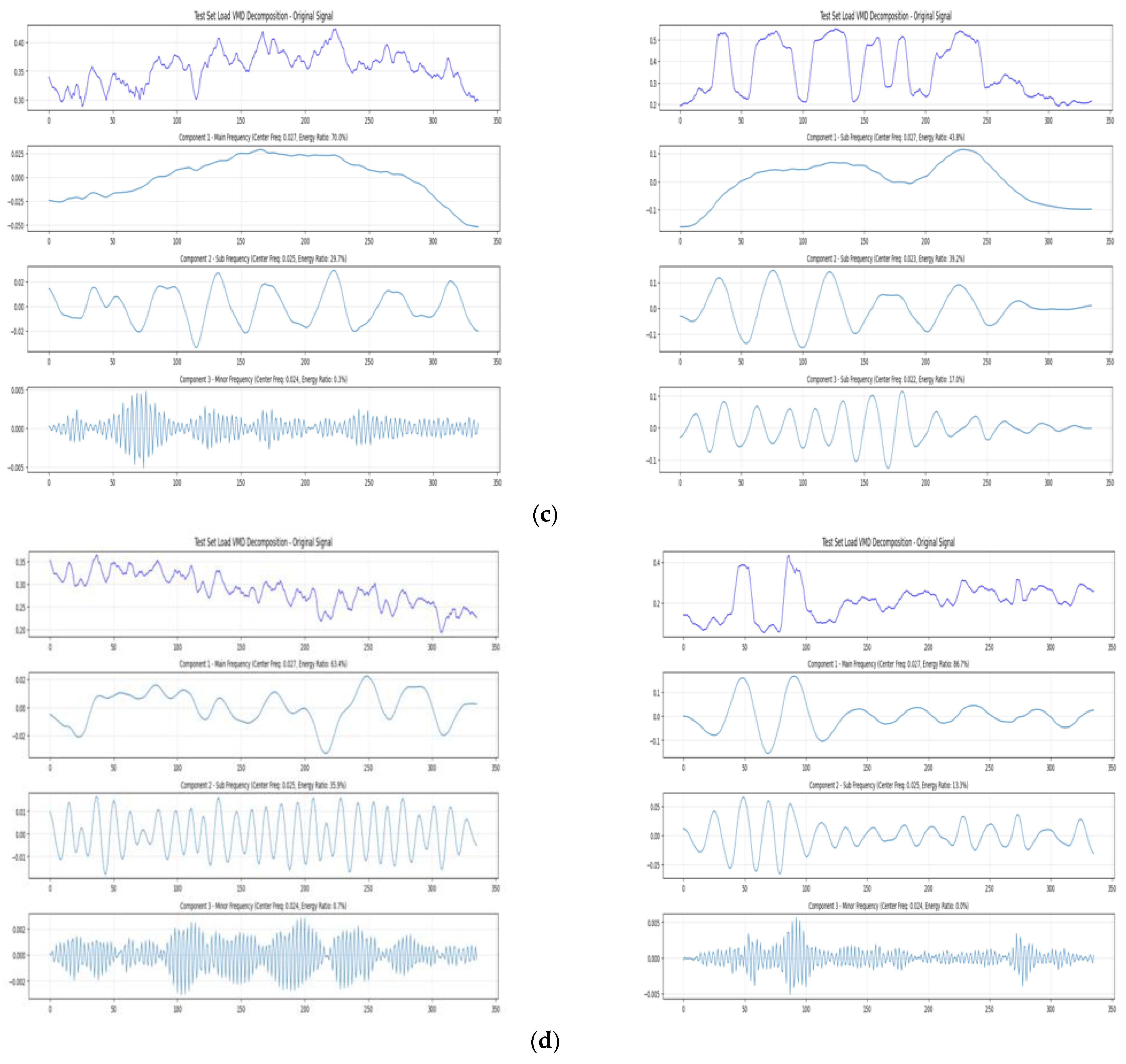
To validate the effectiveness of VMD in extracting multi-scale features from the half-hourly load data of the Ningbo user, we applied VMD decomposition to both the training and test sets of load sequences using the parameters determined in Section 3.2.2. The decomposition resulted in modal components with distinct frequency characteristics and energy distributions. The original power load data for spring, summer, autumn, and winter were successfully decomposed using VMD, with the decomposition results for the test set shown in Figure 5.
From the overall decomposition results, VMD effectively separated the original load sequence into three types of modal components: “dominant frequency component”, “sub-frequency component”, and “minor frequency component”. Moreover, the decomposition patterns were consistent between the training and test sets, demonstrating the stability of VMD in load data preprocessing.
As shown in the figure, the dominant frequency component, serving as the core trend carrier of the load sequence, generally exhibited a high energy proportion, ranging from 63.4% to 89.5% across different scenarios. The sub-frequency component primarily reflected the intraday periodic and short-term fluctuation characteristics of the load, with a secondary energy proportion ranging between 10.3% and 39.2%. In contrast, the minor frequency component often carried random disturbances, with the lowest energy proportion—mostly between 0.2% and 4.4%, and even zero in some scenarios—highlighting its minimal contribution to the overall load energy.

4.2. PSO Optimization Results and Analysis

To enhance the predictive adaptability of LSTM and RF to the various load components decomposed using VMD, we employed the PSO algorithm to intelligently optimize the key hyperparameters of both models. The optimization objective was to maximize the Coefficient of Determination (R2) on the validation set while also balancing the requirements for prediction accuracy and computational efficiency in the electricity spot market. Based on the characteristics of the half-hourly load data from the Ningbo user, the core parameters of the PSO algorithm and the search ranges for the model parameters to be optimized were set. The final optimal parameter combinations obtained are shown in Table 4.
From the overall pattern of the optimization results, the Particle Swarm Optimization (PSO) algorithm fully captured the differentiated characteristics of load data across different seasons. Through seasonally differentiated optimization, the parameter range was extended to an interval more suitable for the half-hourly load data, further verifying the flexibility of PSO in parameter optimization for complex time-series data. To ensure transparency in the training process, the target parameters, constraint conditions, and core training details of PSO optimization were specified as follows:
For the parameters of the PSO algorithm itself: the particle swarm size was set to 30, the maximum number of iterations was 100, the inertia weight adopted a linear decreasing strategy from 0.9 initially to 0.4 at the end, and both the individual and global learning factors were set to 2.0. This configuration balances optimization exploration and convergence efficiency. During the training process, all cases used a batch size of 32 and a training epoch count of 50, with an early stopping strategy implemented. The mean squared error was selected as the loss function, Adam as the optimizer, and He normal distribution for weight initialization—all to enhance the convergence stability and prediction accuracy of the model.
Based on the optimization results in Table 3, the core optimal parameters were determined as follows: the number of hidden layer neurons was 256, the number of stacked layers is 4, the learning rate was 0.01, the number of decision trees was 100, and the maximum depth was 17. This parameter configuration is highly consistent with the parameter range used in short-term load forecasting and achieved a refined adaptation to the seasonal fluctuation characteristics of Ningbo’s half-hourly load [35].
From the perspective of rationality verification: in summer (Case 3, Case 4), due to the high-frequency fluctuations of the load, a lower learning rate and a larger maximum depth of RF were adopted. For the relatively stable loads in winter, spring, and autumn, the learning rate was concentrated around 0.01, and the number of stacked layers was 2–4, balancing the capture of temporal dependencies and the control of model complexity. Meanwhile, the number of hidden layer neurons in LSTM and the number of decision trees in RF were consistent with the parameter intervals reported in existing studies. The seasonally differentiated settings further make up for the poor adaptability of general parameters, rendering the parameter configuration more accurate [36].

4.2.1. Analysis of Seasonal Optimization Results for LSTM Model

The hyperparameters of the LSTM model exhibited significant seasonal adaptation characteristics, as follows:
Number of hidden layer neurons: The optimal values for spring, autumn, and winter were concentrated at 256, while for summer, they were 253 and 224, all within a relatively high range, because the load in Ningbo during spring, autumn, and winter is influenced by both seasonal trends (e.g., winter heating) and peak–valley adjustments in spot electricity prices, resulting in more complex temporal dependencies that require more neurons to capture the coupled characteristics of multiple factors. In contrast, although the summer load experienced cooling demand peaks, its fluctuation patterns were relatively stable (e.g., sustained high load in the afternoon), leading to a slightly lower number of neurons.
Number of stacked layers: Spring and autumn exhibited a 4-layer structure, winter primarily employed 3–4 layers, and summer used 1–2 layers. The load during spring and autumn, given that they are transitional seasons, experienced large intraday fluctuations with no fixed patterns. A 4-layer structure could capture complex temporal dependencies through deep gating mechanisms. Summer load fluctuations were concentrated from afternoon to evening with clear patterns, making 1–2 layers sufficient for adequate fitting. Winter load, affected by continuous heating demand, showed fluctuations intermediate between spring/summer and autumn, thus requiring the employment of 3–4 layers to balance fitting capability and computational efficiency.
Learning rate: Spring, autumn, and winter predominantly used a learning rate of 0.01, while summer employed significantly lower rates of 0.0001 and 0.009661. Summer load data exhibited prominent peaks, where high learning rates can easily cause model oscillations; thus, PSO automatically selected lower learning rates to achieve precise fitting. In contrast, load peaks in other seasons were more moderate, allowing a learning rate of 0.01 to balance convergence speed and accuracy.

4.2.2. Analysis of Seasonal Optimization Results for RF Model

The hyperparameters of the RF model exhibited the characteristic of “stable number of decision trees with seasonal differentiation in maximum depth”, as follows:
The number of decision trees was consistently set to 100 across all four seasons because RF’s core logic of reducing overfitting through multi-tree ensemble is not affected by seasonal variations; thus, 100 trees are sufficient to adequately capture the randomness in load characteristics.
The optimal tree depth ranged from 19–20 for summer and winter while it was 17 for spring and autumn. High temperatures in summer and low temperatures in winter led to stronger nonlinear relationships between load and meteorological factors, requiring deeper tree structures to explore high-dimensional feature correlations. In contrast, the milder meteorological conditions in spring and autumn resulted in more direct relationships between load and features, making a depth of 17 sufficient to avoid overfitting.

4.3. Prediction Result Comparisons

To verify the superiority of the proposed VMD-LSTM-RF hybrid model in the half-hourly load forecasting task for the Ningbo user, we compared the prediction results of the VMD-LSTM-RF model with those of single-model forecasting methods based on the core logic of “component prediction accuracy after decomposition–overall model performance–adaptability to the spot market”. The comparison process refers to an evaluation system of “multi-dimensional metrics + visual validation”, combining the requirements of the electricity spot market for forecasting accuracy. Through comparison charts of predicted versus actual values and key evaluation metric tables, the performance advantages of the model were quantitatively analyzed.

4.3.1. Model Accuracy and Fitting Performance

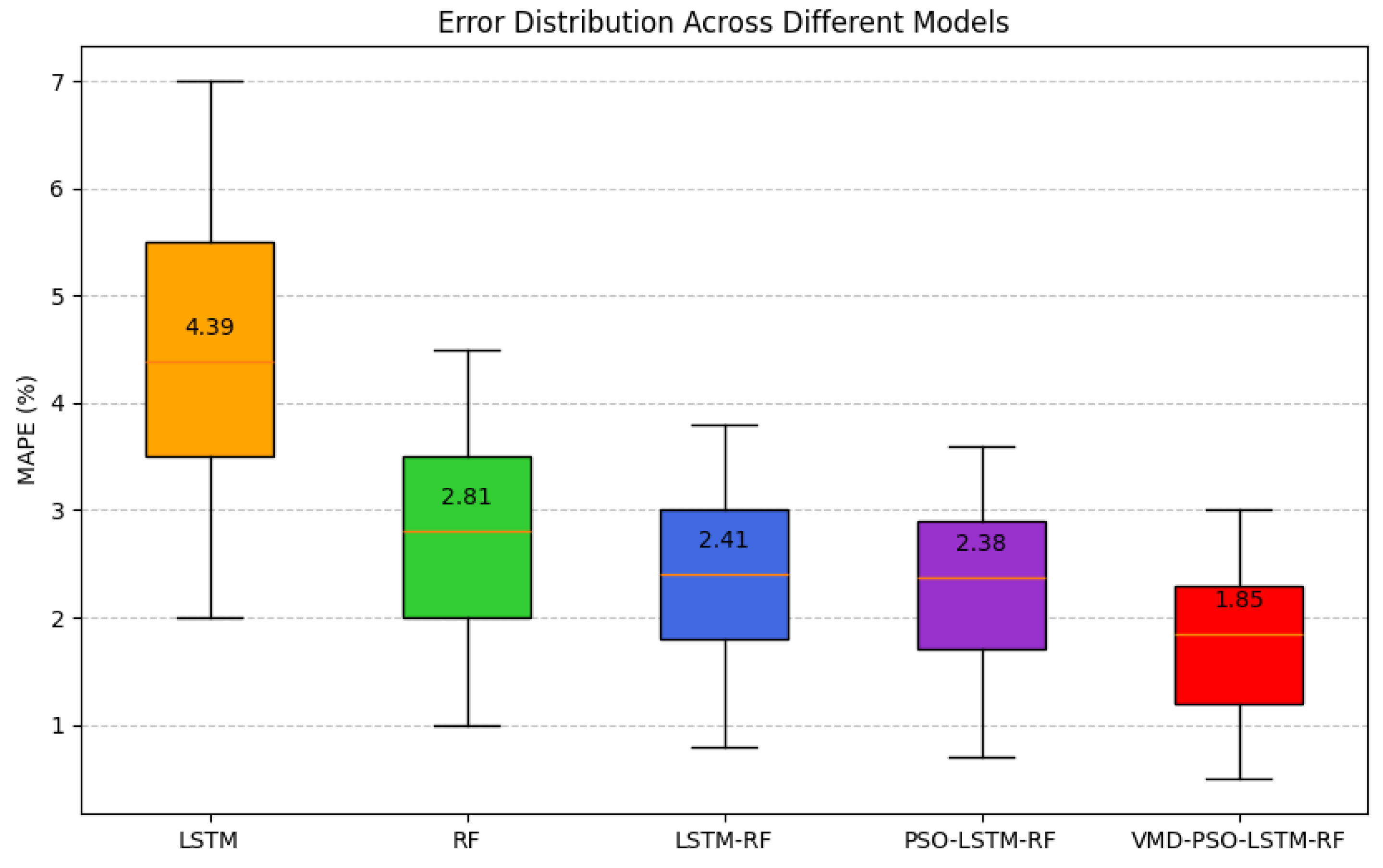
To verify the effectiveness of the proposed VMD-PSO-LSTM-RF model, a multi-model ablation experiment was conducted with summer as an example. The last week of June in the dataset was selected as the test set, and the prediction performances of the LSTM, RF, LSTM-RF, PSO-LSTM-RF, and VMD-PSO-LSTM-RF models were compared. The results are presented in Table 5 and Figure 6.
As can be seen from the quantitative indicators in Table 5, the VMD-PSO-LSTM-RF model performed optimally in terms of R2 (0.9520), MAPE (1.85%), RMSE (0.0098), and MAE (1.83): compared with the single LSTM model, its R2 was increased by 8.69% and MAPE was reduced by 57.53%; compared with the RF model, its R2 was increased by 3.08% and MAPE was reduced by 34.07%; even when compared with the PSO-LSTM-RF model without VMD decomposition, its R2 still increased by 0.75% and MAPE decreased by 19.08%. Combined with the boxplot of error distribution in Figure 6, the MAPE box of the VMD-PSO-LSTM-RF model was the narrowest with the lowest median, indicating that the concentration and stability of its prediction errors were significantly superior to those of other models.
The core logic for selecting the VMD-PSO-LSTM-RF model lies in the synergistic gain of each module: VMD separates the trend, periodic, and random features of the load through multi-scale decomposition, providing purer inputs for subsequent modeling; PSO performs global optimization on the hyperparameters of LSTM and RF, solving the limitation that model parameters rely on empirical settings; the integrated modeling of LSTM and RF captures both the temporal dependencies of the load and the multi-feature correlation patterns, which provides an efficient and accurate solution for short-term load forecasting of comprehensive multi-industry users.
Restricted by data acquisition conditions, to maximize the sample size of the training set and improve the generalization ability of the model, this study constructed a cyclic data sequence by connecting the data of 12 consecutive months end-to-end. On this basis, the test set and training set were divided by season. This division method does not change the authenticity and seasonal characteristics of the data itself, and only avoids model overfitting caused by insufficient sample size through cyclic expansion.
To verify the robustness of the proposed VMD-PSO-LSTM-RF model, two weeks of data per month in summer were selected as the test set, and multiple groups of robustness tests were conducted. The results are shown in Table 6.
As can be seen from the results in the table, the model maintained high prediction stability across the test sets of different weeks: the R2 values stably ranged from 0.9638 to 0.9799, the MAPE values were concentrated between 0.61% and 1.86%, and although the RMSE values fluctuated due to differences in monthly load scales, they were generally within a reasonable range. This performance confirms the model’s adaptability to load data from different time periods in summer and also demonstrates the rationality of the strategy of constructing the training set by cycling one year of data. Even though the training set included cyclic data from future time periods, the model could still maintain stable accuracy across different test sets by capturing the seasonal and weekly characteristics of the load. No overfitting or prediction deviation was caused by data cycling, which further verifies the scientificity of the data division method and the robustness of the model.
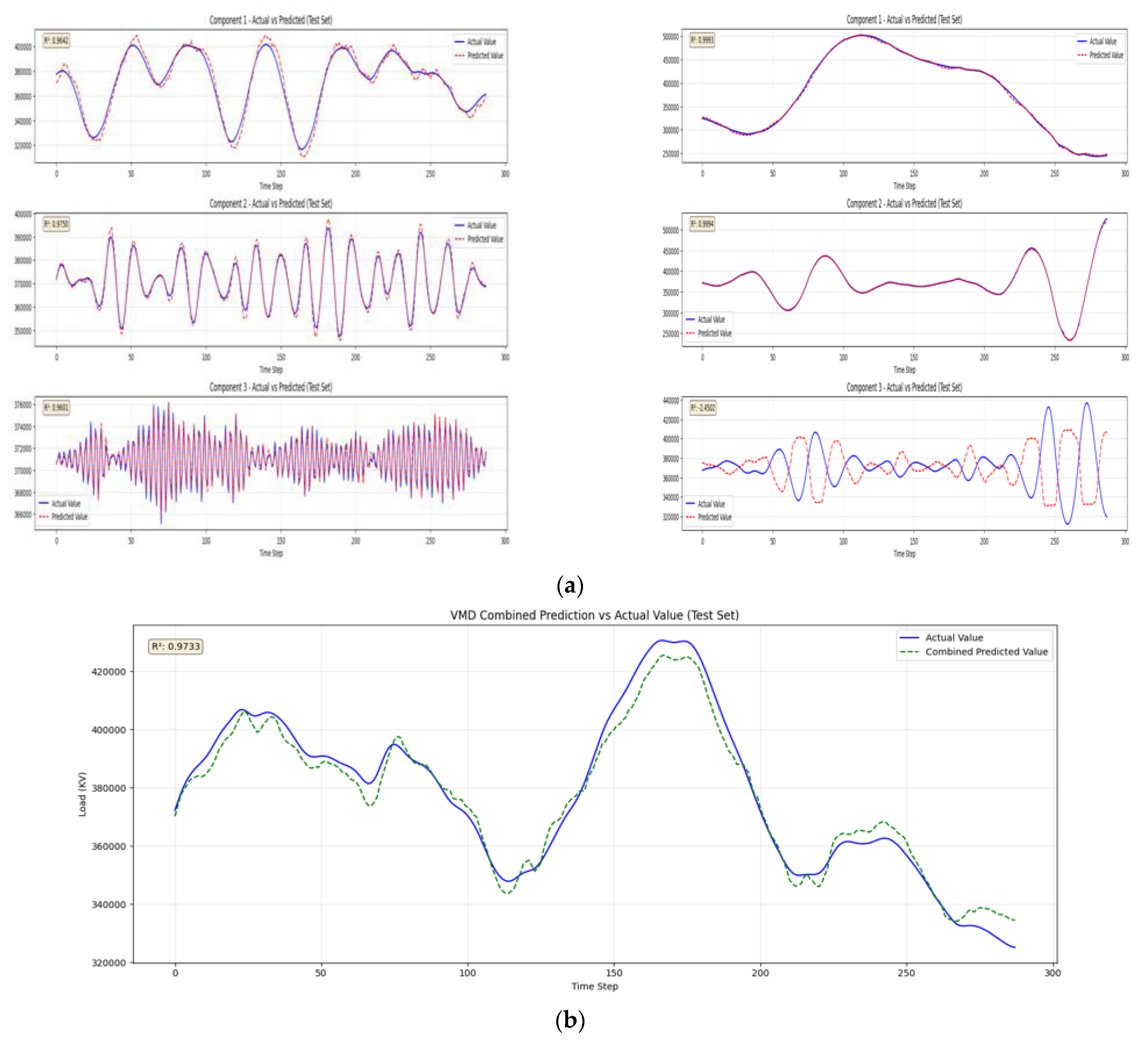
Taking summer load forecasting as an example, the summer load forecast is shown in Figure 7.
From the comparative charts of individual components and comprehensive forecasting for summer, the VMD-LSTM-RF model demonstrated excellent fitting performance. At the component-forecasting level:
  • The dominant frequency component reflects the main trend of the load;
  • The sub-frequency component captures intraday periodic characteristics;
  • The minor frequency component carries random disturbances.
All of these components showed prediction curves that closely aligned with the actual values, with R2 values mostly above 0.96. Only the minor frequency component exhibited a slightly lower R2 in certain periods due to the difficulty in fitting random disturbances.
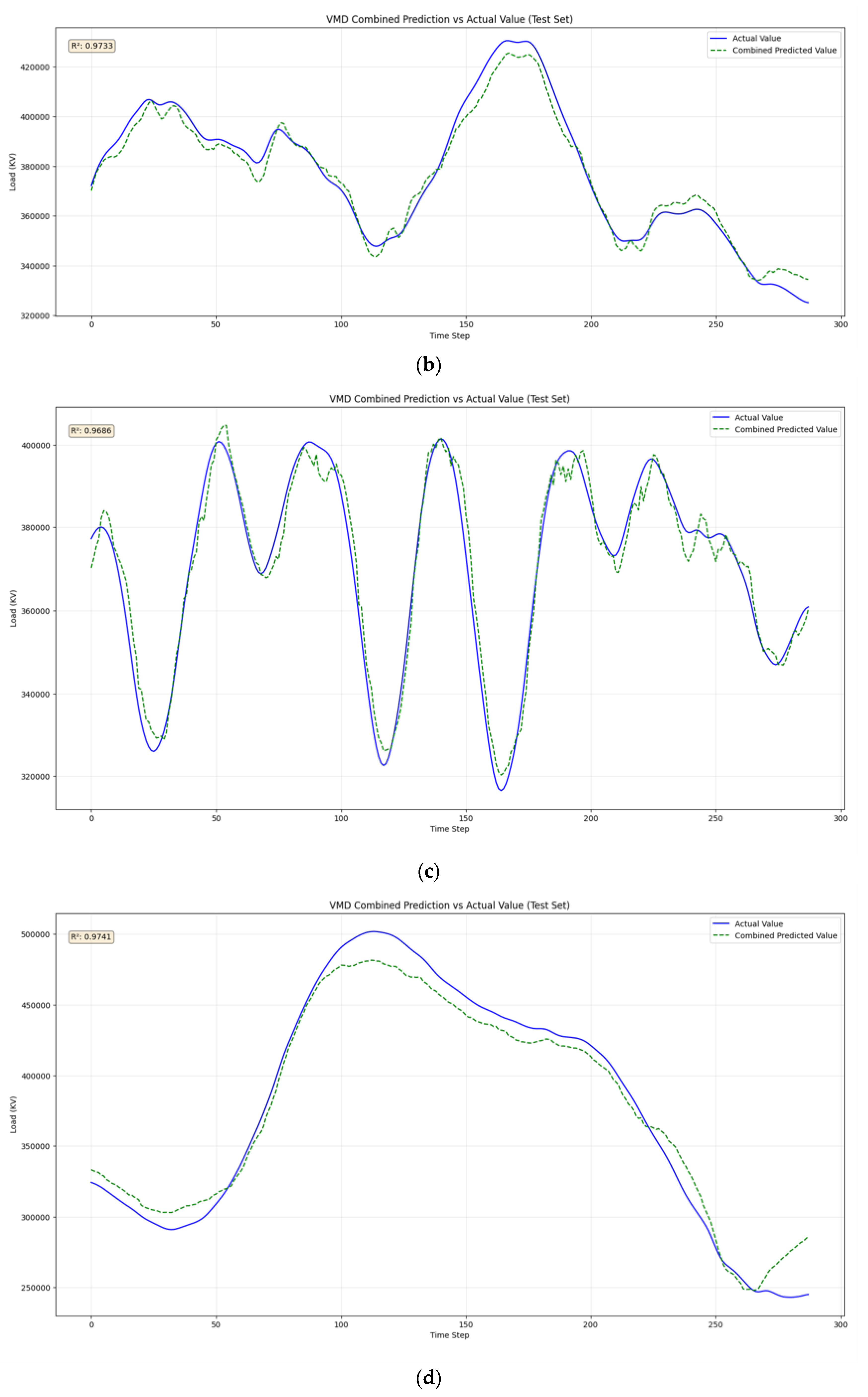
In the comprehensive forecasting chart, the model’s prediction curve closely followed the fluctuations of the actual load curve; particularly, during periods of high peak loads and significant fluctuations in summer, the model accurately captured the rising and falling trends of the load. The R2 values reached 0.9686 and 0.9741, fully indicating the model’s high degree of fit to the complex load variation characteristics in summer and the strong consistency between the predicted and actual values, providing reliable forecasting support for decision making in the electricity market during summer periods.

4.3.2. Seasonal Adaptability

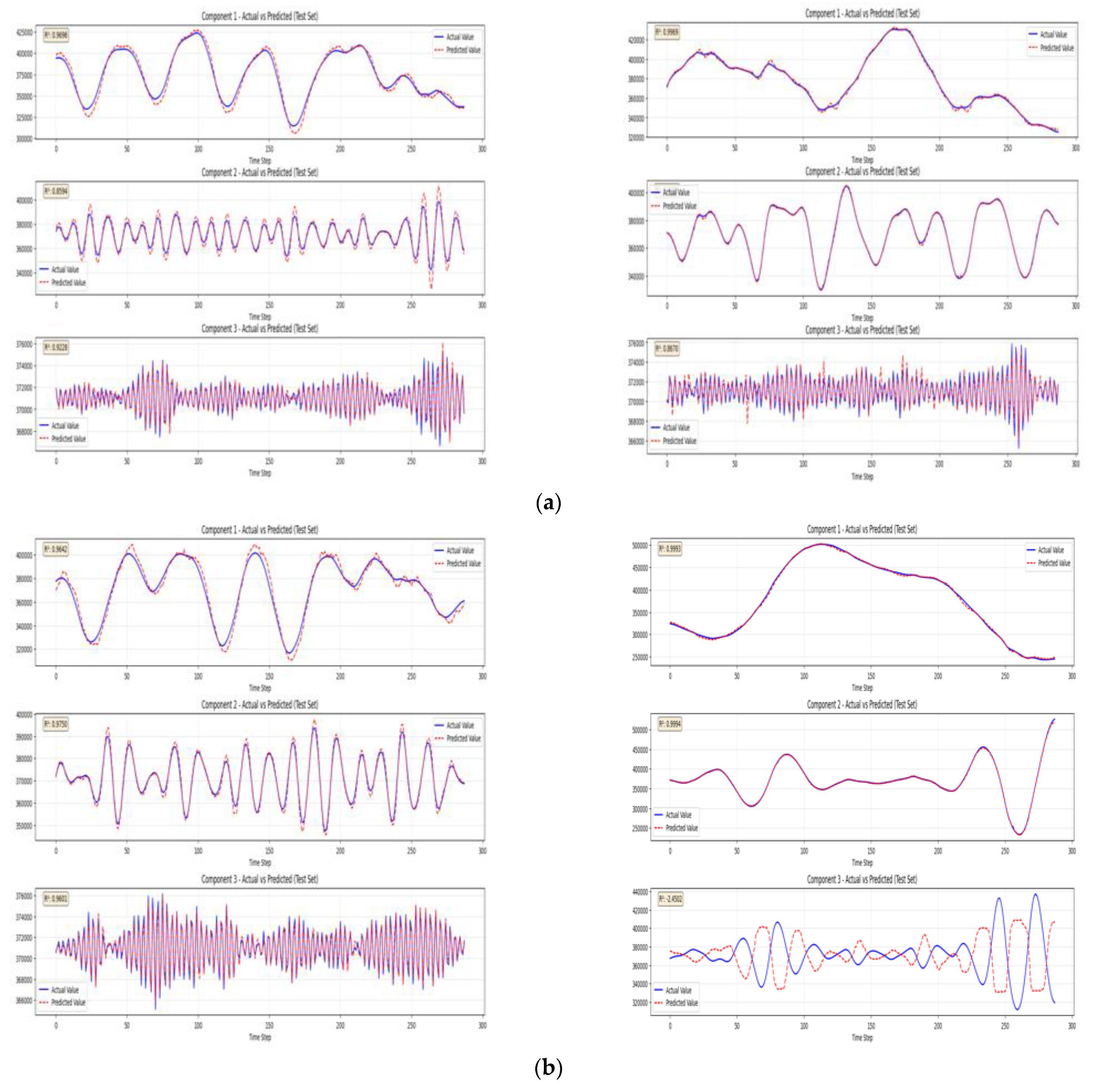
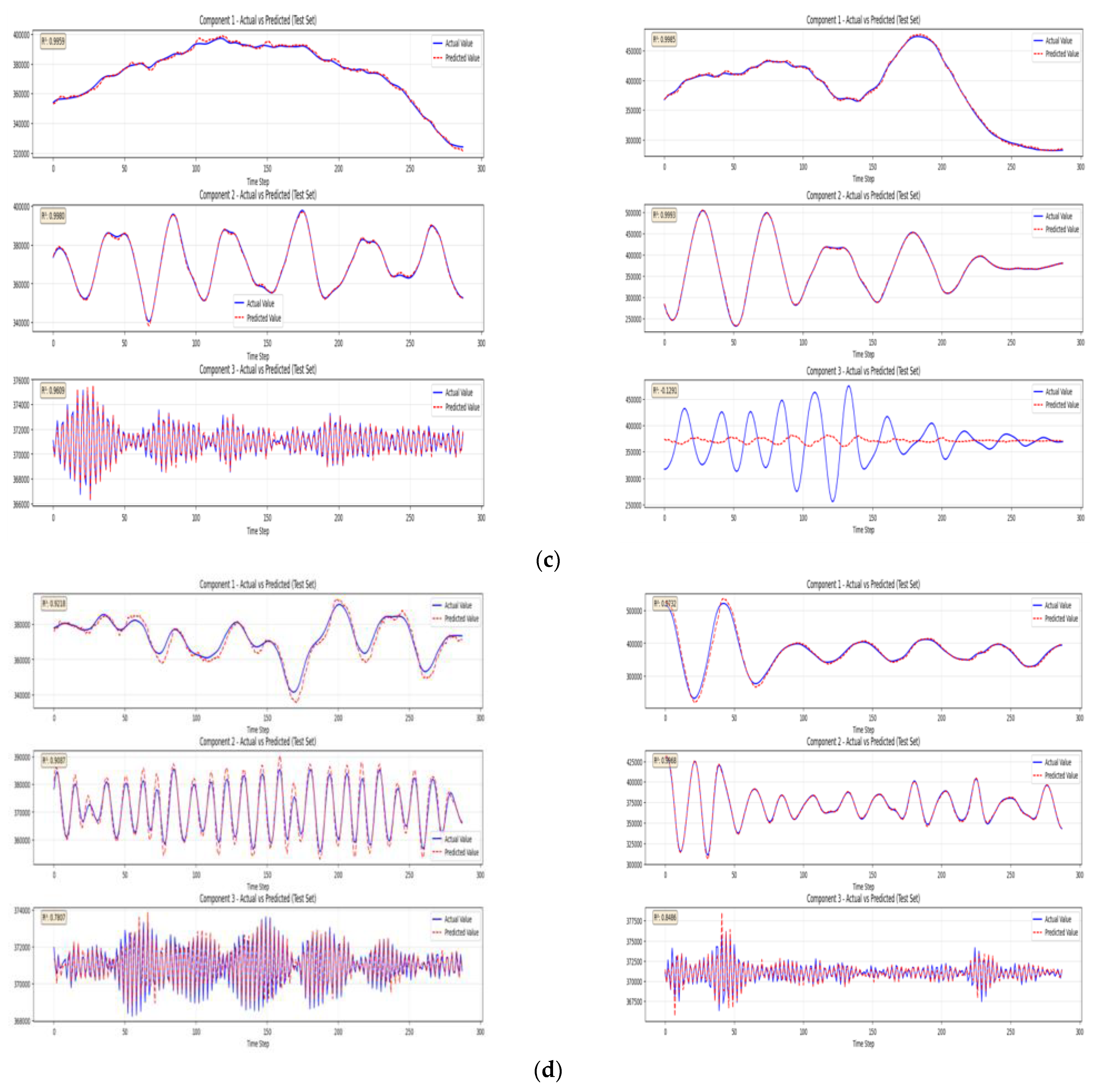
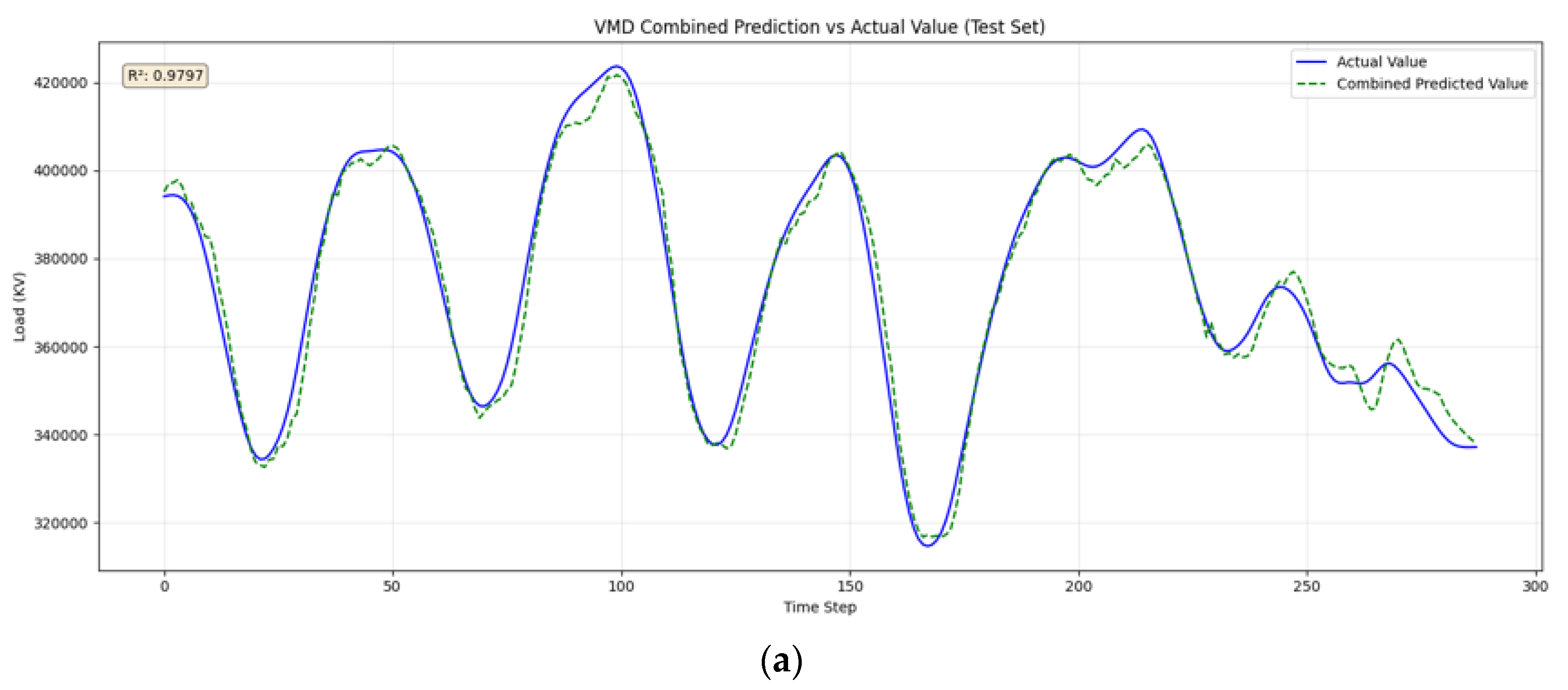
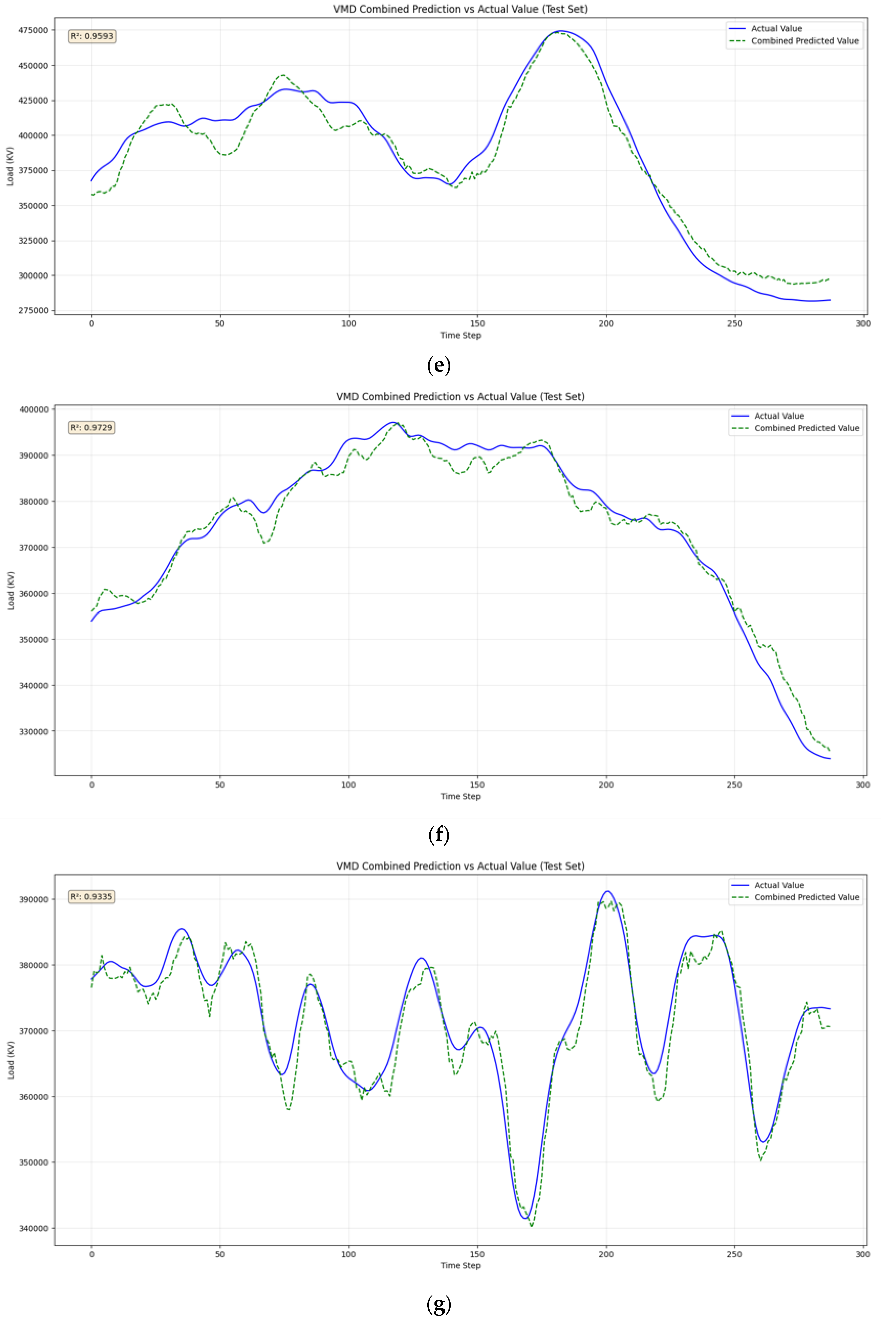
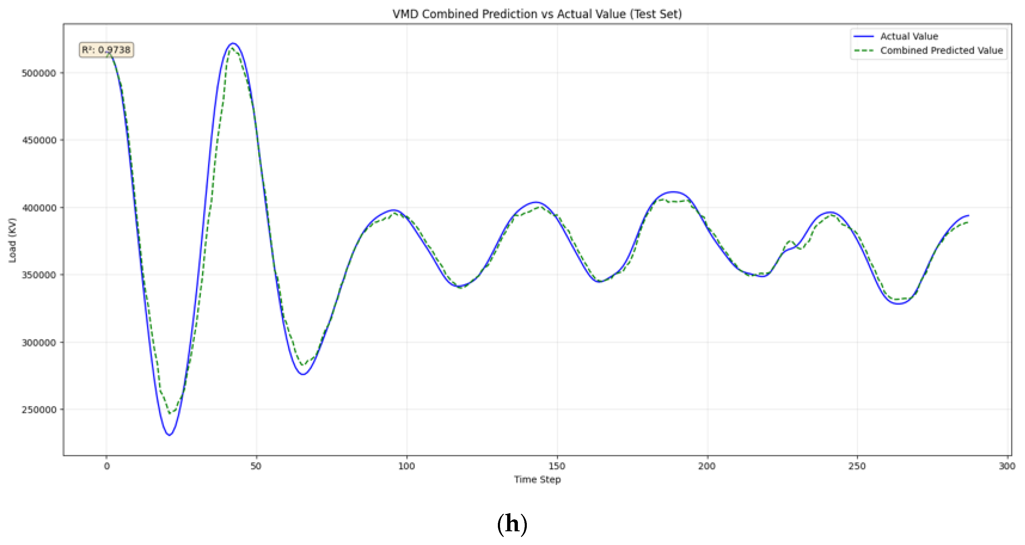
The VMD-LSTM-RF hybrid model demonstrated excellent seasonal adaptability in the half-hourly load forecasting task for the Ningbo user, which stems from its three-tier collaborative architecture of “signal decomposition–temporal modeling–ensemble optimization,” and its performance across different seasons can be validated through key evaluation metrics and visualized forecasting results. The comparison between the predicted and actual values of each modal component after VMD decomposition is shown in Figure 8, and the forecasting results of the VMD-LSTM-RF model are presented in Figure 9.
From the perspective of signal preprocessing, the introduction of Variational Mode Decomposition (VMD) serves as the foundational prerequisite for accuracy improvement and seasonal adaptability. Raw load data exhibit strong non-stationarity due to the integration of multiple features such as seasonal trends, intraday cycles, and random disturbances, making it difficult for a single LSTM-RF model to simultaneously adapt to multi-scale fluctuations; in contrast, VMD adaptively decomposes the original sequence into modal components with distinct frequency characteristics by constructing a constrained variational model. As evident from the component prediction charts for spring, summer, autumn, and winter, the decomposed dominant, sub-, and minor frequency components achieved feature decoupling; thus, this approach effectively overcomes the mode mixing issue inherent in traditional EMD, providing subsequent models with high-quality, “denoised and multi-scale” inputs, enabling the models to better capture the core characteristics of load data across different seasons.
However, during one specific week of winter data, the R2 decreased to around 0.93 after applying VMD, indicating a reduction in accuracy. The speculated reason is that when the load data for that week exhibited extremely weak multi-scale fluctuation characteristics, almost resembling a single-domain feature, VMD decomposition may have over-split the original data, introducing unnecessary decomposition errors that subsequently impacted the learning performance of the downstream models.
From the perspective of predictive module synergy, the combination of LSTM and RF achieves complementary advantages, enabling the model to adapt to seasonal variations. The gating mechanism of LSTM naturally aligns with the temporal dependencies of load data, allowing it to accurately capture long-term trends, such as the gentle fluctuations in spring and the sustained peak heating loads in winter. In contrast, the ensemble learning characteristic of RF exhibits strong robustness against random disturbances, effectively fitting short-term fluctuations caused by summer thunderstorms or autumn seasonal transitions. A comparison of the comprehensive forecasting charts across the four seasons revealed that single VMD component predictions showed significant lag during high-frequency fluctuation periods; however, the VMD-LSTM-RF model, by leveraging LSTM to learn temporal patterns and RF to optimize detailed deviations, significantly improved the alignment between the predicted curve and actual values.
A comparison of key evaluation metrics is shown in Table 7.
Based on the comparison table of key evaluation metrics, the model demonstrated outstanding performance across all four seasons, with R2 mostly above 0.95, RMSE ranging approximately between 3000 and 13,000, and MAPE within a relatively low range of 0.68–2.58. Compared with the LSTM-RF model, the VMD-LSTM-RF model achieved higher R2 and lower RMSE and MAPE values in all seasons, fully showcasing its strong adaptability to load characteristics and effective prediction under different seasonal conditions, whether they are gentle fluctuations in spring, high peak variations in summer, the trend transitions in autumn, or the sustained peaks and troughs in winter.

4.3.3. Electricity Market Application Value

In the electricity market, the accuracy of load forecasting directly impacts power generation planning, electricity price adjustments, and user consumption strategies. The high-precision forecasting of the VMD-LSTM-RF model brings multifaceted value, as follows:
Generation side: More accurate load forecasting enables optimized power generation planning, reducing wasted reserve capacity and emergency peak-shaving costs, thereby improving the power generation efficiency.
Electricity trading institutions: Based on precise load forecasting, day-ahead market clearing prices can be calculated more accurately, mitigating market trading risks and enhancing the efficiency and stability of electricity spot market transactions.
User side: With accurate peak and valley load forecasting, users can better arrange bidding and consumption strategies, capture peak–valley price differentials, optimize load curves, and reduce electricity costs.
In summary, the VMD-LSTM-RF model, which preprocesses load data using Variational Mode Decomposition (VMD) and combines the strengths of Long Short-Term Memory (LSTM) and Random Forest (RF), significantly outperforms the LSTM-RF model regarding the load forecasting accuracy, seasonal adaptability, and electricity market application value, providing robust technical support for the efficient operation of power systems and the sound development of electricity markets.

5. Conclusions

In this study, we addressed the high-precision requirements of load forecasting in electricity markets and tackled the non-stationary and nonlinear challenges of Short-Term Load Forecasting (STLF) in power systems. We proposed a hybrid forecasting model based on VMD, LSTM, and RF, combined with the PSO algorithm to optimize model hyperparameters. Using half-hourly load data from a Ningbo user as the research subject, an empirical analysis was conducted, leading to the following conclusions:
(1) The model significantly improved the short-term load forecasting accuracy through VMD decomposition and collaborative model architecture. Compared with the LSTM-RF model, the R2 values on the test sets across the four seasons showed overall improvement of 2.1% to 5.9%; the RMSE values were reduced by an average of 42.3% to 58.7%, and the MAPE value decreased by an average of 0.15 to 1.61 percentage points, with more stable prediction errors across seasons.
(2) The model demonstrated strong adaptability to load characteristics across different seasons. Addressing the seasonal variations in the Ningbo area—such as gentle fluctuations in spring, high peak values and volatility in summer, trend transitions in autumn, and sustained heating peaks in winter—the model utilizes VMD to adaptively decompose the load of each season into dominant, secondary, and minor frequency components. By combining LSTM’s ability to capture temporal trends with RF’s robustness against random disturbances, the model maintains excellent forecasting performance throughout all four seasons.
(3) The high-precision forecasting capability of the proposed model can support multi-agent decision making in electricity markets, providing technical support for the efficient operation of electricity spot markets. Simultaneously, it offers a methodological framework that can be referenced for load forecasting in similar regions.

Author Contributions

Conceptualization, L.Y. and L.S. (Lifei Song); Methodology, K.L., F.Q., X.W., L.W., J.D. and L.S. (Lianyi Shen); Formal analysis, K.L., L.Y. and L.S. (Lifei Song); Investigation, F.Q., X.W., L.W., J.D. and L.S. (Lianyi Shen); Data curation, L.Y. and L.S. (Lifei Song); Writing–original draft, K.L., L.Y. and L.S. (Lifei Song); Writing–review & editing, K.L., F.Q., X.W., L.W., J.D. and L.S. (Lianyi Shen); Funding acquisition, K.L. All authors have read and agreed to the published version of the manuscript.

Funding

This research was funded by China Energy Zhejiang Energy Sales Co., Ltd. grant number GNZX-FW-2025-7 And The APC was funded by Shanghai University of Electric Power.

Data Availability Statement

The raw data supporting the conclusions of this article will be made available by the authors on request.

Conflicts of Interest

Authors Kangkang Li, Li Wang, Jiefen Dai and Lianyi Shen were employed by the company China Energy Zhejiang Energy Sales Co., Ltd. Author Xinhong Wu was employed by the company State Grid Zhejiang Integrated Energy Service Company. The remaining authors declare that the research was conducted in the absence of any commercial or financial relationships that could be construed as a potential conflict of interest. This study received funding from China Energy Zhejiang Energy Sales Co. Ltd. The funder provided the data and relevant materials for this research. All authors were involved in the study and have contributed to the manuscript.

Abbreviations

SVRSupport Vector Regression
LSTMLong Short-Term Memory
RFRandom Forest
EMDEmpirical Mode Decomposition
VMDVariational Mode Decomposition
MODBOMulti-Objective Dark Bandit Optimizer
SVDSingular Value Decomposition
RNNRecurrent Neural Network
ANNArtificial Neural Network
MTLMulti-Task Learning
SSASparrow Search Algorithm
EEMDEnsemble Empirical Mode Decomposition
SVMDSparse Variational Mode Decomposition
IZOAImproved Zebra Optimization Algorithm
IMFIntrinsic Mode Function
GRUGated Recurrent Unit

References

  1. Wang, G.; Chen, X. Power System Load Forecasting Based on Multiple Models. Adv. Appl. Math. 2024, 13, 750–759. [Google Scholar] [CrossRef]
  2. Tarmanini, C.; Sarma, N.; Gezegin, C.; Ozgonenel, O. Short term load forecasting based on ARIMA and ANN approaches. Energy Rep. 2023, 9 (Suppl. S3), 550–557. [Google Scholar] [CrossRef]
  3. Lu, R.; Bai, R.; Li, R.; Zhu, L.; Sun, M.; Xiao, F.; Wang, D.; Wu, H.; Ding, Y. A Novel Sequence-to-Sequence-Based Deep Learning Model for Multistep Load Forecasting. IEEE Trans. Neural Netw. Learn. Syst. 2025, 36, 638–652. [Google Scholar] [CrossRef] [PubMed]
  4. Ortega, A.; Borunda, M.; Conde, L.; Garcia-Beltran, C. Load Demand Forecasting Using a Long-Short Term Memory Neural Network. In Advances in Computational Intelligence; Calvo, H., Martínez-Villaseñor, L., Ponce, H., Eds.; MICAI 2023; Lecture Notes in Computer Science; Springer: Cham, Switzerland, 2024; Volume 14391. [Google Scholar]
  5. Li, K.; Huang, W.; Hu, G.; Li, J. Ultra-short term power load forecasting based on CEEMDAN-SE and LSTM neural network. Energy Build. 2023, 279, 112666. [Google Scholar] [CrossRef]
  6. Cao, Z.; Wang, J.; Xia, Y. Combined electricity load-forecasting system based on weighted fuzzy time series and deep neural networks. Eng. Appl. Artif. Intell. 2024, 132, 108375. [Google Scholar] [CrossRef]
  7. Luo, S.; Wang, B.; Gao, Q.; Wang, Y.; Pang, X. Stacking integration algorithm based on CNN-BiLSTM-Attention with XGBoost for short-term electricity load forecasting. Energy Rep. 2024, 12, 2676–2689. [Google Scholar] [CrossRef]
  8. Zhang, S.; Chen, R.; Cao, J.; Tan, J. A CNN and LSTM-based multi-task learning architecture for short and medium-term electricity load forecasting. Electr. Power Syst. Res. 2023, 222, 109507. [Google Scholar] [CrossRef]
  9. Li, J.; Qiu, C.; Zhao, Y.; Wang, Y. A power load forecasting model based on a combined neural network. AIP Adv. 2024, 14, 045231. [Google Scholar] [CrossRef]
  10. Deng, S.; Dong, X.; Tao, L.; Wang, J.; He, Y.; Yue, D. Multi-type load forecasting model based on random forest and density clustering with the influence of noise and load patterns. Energy 2024, 307, 132635. [Google Scholar] [CrossRef]
  11. Guerra, R.R.; Vizziello, A.; Savazzi, P.; Goldoni, E.; Gamba, P. Forecasting LoRaWAN RSSI using weather parameters: A comparative study of ARIMA, artificial intelligence and hybrid approaches. Comput. Netw. 2024, 243, 110258. [Google Scholar] [CrossRef]
  12. Lv, L.; Wu, Z.; Zhang, J.; Zhang, L.; Tan, Z.; Tian, Z. A VMD and LSTM Based Hybrid Model of Load Forecasting for Power Grid Security. IEEE Trans. Ind. Inform. 2022, 18, 6474–6482. [Google Scholar] [CrossRef]
  13. Duo, Y.; Li, W.; Li, T. Short Term Power Load Forecasting Based on VMD Self Attention-LSTM. Adv. Appl. Math. 2023, 12, 1195–1206. [Google Scholar] [CrossRef]
  14. Dai, Y.; Yu, W. Short-term power load forecasting based on Seq2Seq model integrating Bayesian optimization, temporal convolutional network and attention. Appl. Soft Comput. 2024, 166, 112248. [Google Scholar] [CrossRef]
  15. Chen, J.; Liu, L.; Guo, K.; Liu, S.; He, D. Short-Term Electricity Load Forecasting Based on Improved Data Decomposition and Hybrid Deep-Learning Models. Appl. Sci. 2024, 14, 5966. [Google Scholar] [CrossRef]
  16. Li, Y. Short-Term Power Load Forecasting Modeling Based on Transfer Fuzzy System. Adv. Appl. Math. 2024, 13, 1671–1689. [Google Scholar] [CrossRef]
  17. Yang, M.; Guo, Z.; Wang, D.; Wang, B.; Wang, Z.; Huang, T. Short-term photovoltaic power forecasting method considering historical information reuse and numerical weather forecasting. Renew. Energy 2025, 256, 123933. [Google Scholar] [CrossRef]
  18. Wang, T.; Sun, J.; Gong, D.; Wang, F.; Yue, F. A Dual-layer Decomposition and Multi-model Driven Combination Interval Forecasting Method for Short-term PV Power Generation. Expert Syst. Appl. 2025, 288, 128235. [Google Scholar] [CrossRef]
  19. Liu, R.; Shi, J.; Sun, G.; Lin, S.; Li, F. A Short-term net load hybrid forecasting method based on VW-KA and QR-CNN-GRU. Electr. Power Syst. Res. 2024, 232, 110384. [Google Scholar] [CrossRef]
  20. Li, C.; Li, G.; Wang, K.; Han, B. A multi-energy load forecasting method based on parallel architecture CNN-GRU and transfer learning for data deficient integrated energy systems. Energy 2022, 259, 124967. [Google Scholar] [CrossRef]
  21. Niu, D.; Yu, M.; Sun, L.; Gao, T.; Wang, K. Short-term multi-energy load forecasting for integrated energy systems based on CNN-BiGRU optimized by attention mechanism. Appl. Energy 2022, 313, 118801. [Google Scholar] [CrossRef]
  22. Tan, M.; Liao, C.; Chen, J.; Cao, Y.; Wang, R.; Su, Y. A multi-task learning method for multi-energy load forecasting based on synthesis correlation analysis and load participation factor. Appl. Energy 2023, 343, 121177. [Google Scholar] [CrossRef]
  23. Huang, N.; Ren, S.; Liu, J.; Cai, G.; Zhang, L. Multi-task learning and single-task learning joint multi-energy load forecasting of integrated energy systems considering meteorological variations. Expert Syst. Appl. 2025, 288, 128269. [Google Scholar] [CrossRef]
  24. Li, K.; Mu, Y.; Yang, F.; Wang, H.; Yan, Y.; Zhang, C. Joint forecasting of source-load-price for integrated energy system based on multi-task learning and hybrid attention mechanism. Appl. Energy 2024, 360, 122821. [Google Scholar] [CrossRef]
  25. Lin, Z.; Lin, T.; Li, J.; Li, C. A novel short-term multi-energy load forecasting method for integrated energy system based on two-layer joint modal decomposition and dynamic optimal ensemble learning. Appl. Energy 2025, 378, 124798. [Google Scholar] [CrossRef]
  26. Ren, X.; Tian, X.; Wang, K.; Yang, S.; Chen, W.; Wang, J. Enhanced load forecasting for distributed multi-energy system: A stacking ensemble learning method with deep reinforcement learning and model fusion. Energy 2025, 319, 135031. [Google Scholar] [CrossRef]
  27. Peng, D.; Liu, Y.; Wang, D.; Zhao, H.; Qu, B. Multi-energy load forecasting for integrated energy system based on sequence decomposition fusion and factors correlation analysis. Energy 2024, 308, 132796. [Google Scholar] [CrossRef]
  28. Zhang, Y.; Wu, P.; Ma, X.; Qian, X. Short Term Load Forecasting Method for Power System Based on Neural Network. In Proceedings of the 2024 5th International Symposium on New Energy and Electrical Technology (ISNEET), Hangzhou, China, 27–29 December 2024; pp. 481–484. [Google Scholar] [CrossRef]
  29. Xu, Y.; Yang, J.; Cai, X. Intelligent analysis algorithm for power engineering data based on improved BiLSTM. Sci. Rep. 2025, 15, 15320. [Google Scholar] [CrossRef]
  30. Al-Selwi, S.M.; Hassan, M.F.; Abdulkadir, S.J.; Muneer, A.; Sumiea, E.H.; Alqushaibi, A.; Ragab, M.G. RNN-LSTM: From applications to modeling techniques and beyond—Systematic review. J. King Saud Univ.—Comput. Inf. Sci. 2024, 36, 102068. [Google Scholar] [CrossRef]
  31. Yue, W.; Liu, Q.; Ruan, Y.; Qian, F.; Meng, H. A prediction approach with mode decomposition-recombination technique for short-term load forecasting. Sustain. Cities Soc. 2022, 85, 104034. [Google Scholar] [CrossRef]
  32. Ou, H.; Yao, Y.; He, Y. Missing Data Imputation Method Combining Random Forest and Generative Adversarial Imputation Network. Sensors 2024, 24, 1112. [Google Scholar] [CrossRef]
  33. Rani, S.; Mahmood, A.; Ahmed, U.; Razzaq, S.; Manzoor, S. A Short-Term Load Forecasting by Using Hybrid Model. In Proceedings of the 2023 20th International Bhurban Conference on Applied Sciences and Technology (IBCAST), Bhurban, Pakistan, 22–25 August 2023; pp. 333–338. [Google Scholar] [CrossRef]
  34. Xu, Y.; Huang, X.; Zheng, X.; Zeng, Z.; Jin, T. VMD-ATT-LSTM electricity price prediction based on grey wolf optimization algorithm in electricity markets considering renewable energy. Renew. Energy 2024, 236, 121408. [Google Scholar] [CrossRef]
  35. Peng, S.; Zhu, J.; Wu, T.; Yuan, C.; Cang, J.; Zhang, K.; Pecht, M. Prediction of wind and PV power by fusing the multi-stage feature extraction and a PSO-BiLSTM model. Energy 2024, 298, 131345. [Google Scholar] [CrossRef]
  36. Bo, Y.; Guo, X.; Liu, Q.; Pan, Y.; Zhang, L.; Lu, Y. Prediction of tunnel deformation using PSO variant integrated with XGBoost and its TBM jamming application. Tunn. Undergr. Space Technol. 2024, 150, 105842. [Google Scholar] [CrossRef]
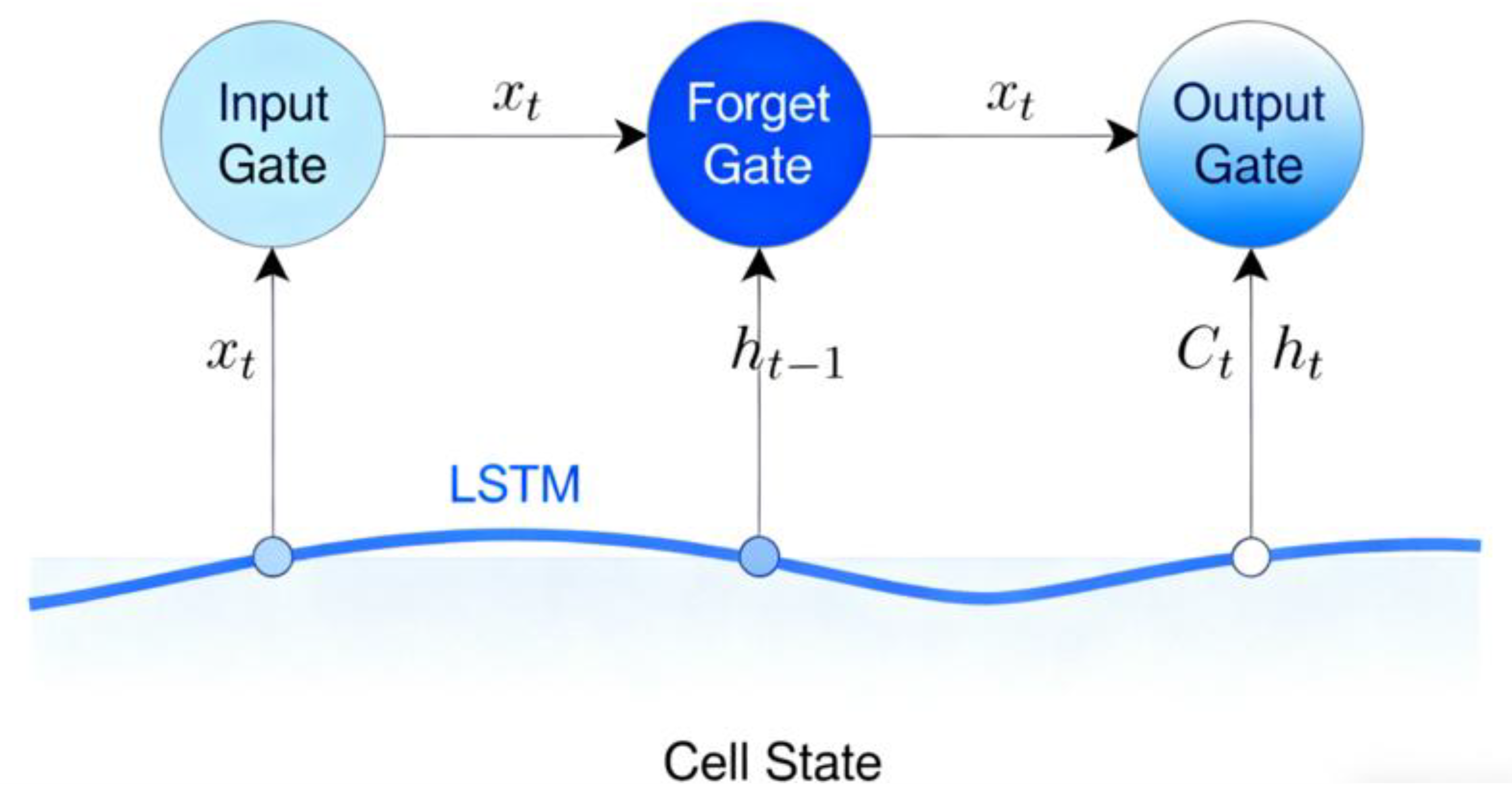
Figure 1. LSTM Structure.
Energies 18 06097 g001
Figure 2. Workflow of the VMD-PSO-LSTM-RF Combined Forecasting Model.
Energies 18 06097 g002
Figure 3. Time Series of Initial Power Load.
Energies 18 06097 g003
Figure 4. The load proportion of different industries.
Energies 18 06097 g004
Figure 5. VMD Decomposition Results of Power Load for (a) Spring, (b) Summer, (c) Autumn, and (d) Winter.
Energies 18 06097 g005aEnergies 18 06097 g005b
Figure 6. Error Distribution of Multi-Model Ablation Experiments.
Energies 18 06097 g006
Figure 7. (a) Modal Components After VMD Decomposition. (b) Summer Load Forecasting Chart of VMD-LSTM-RF Model.
Energies 18 06097 g007
Figure 8. Comparison of Predicted and Actual Values of Modal Components after VMD Decomposition for (a) Spring, (b) Summer, (c) Autumn, and (d) Winter.
Energies 18 06097 g008aEnergies 18 06097 g008b
Figure 9. VMD-LSTM-RF Model Prediction Results for (a,b) Spring, (c,d) Summer, (e,f) Autumn, and (g,h) Winter.
Energies 18 06097 g009aEnergies 18 06097 g009bEnergies 18 06097 g009cEnergies 18 06097 g009d
Table 1. Summary of Existing Load Forecasting Models.
ScenarioInput VariablesModelTraining TimeRefs
Load ForecastingIoT data, historical load data, meteorological data, economic data, historical load data, meteorological data, time featuresLSTM, LSTM-GRU, Stacking-Fusion, Reseamble-ModelMedium–Long[17,18]
IoT data, historical load data, meteorological data, economic dataShuffle-Transformer-Multi, Transformer-Attention-NetRelatively Long[3,19]
Historical load data, meteorological data, time features, multi-energy load dataCNN-LSTM, CNN-BiGRU, ResNet-LSTMMedium–Long[8,20,21]
Historical load data, meteorological data, multi-energy data, coupling featuresMulti-task Learning, Source-Load Integrated Forecasting ModelRelatively Long[22,23,24]
Historical load data, meteorological data, multi-energy data, key featuresTwo-layer Joint Modal Decomposition Dynamic Ensemble Model, Stacking Ensemble, Copula Correlation Analysis FusionLong[25,26,27]
Table 2. VMD Parameter Settings.
TypeParameterRage
Dynamic adaptable parametersNumber of Decomposition Modes3
Penalty Factor2000
Basic fixed parametersNoise Tolerance0
Whether to Enforce DC Component Decomposition0
Center Frequency Initialization Method1
Convergence Threshold10−7
Table 3. PSO Parameter Settings.
TypeParameterRage
Core Algorithm ParametersNumber of Particles20
Maximum Iterations40
Inertia Weight0.9
Cognitive and Social Coefficients2.0
Model Parameter Rangers to Be OptimizedNumber of Hidden Layer Neurons[32,256]
Number of Stacked Layers[1,5]
Learning Rate[0.0001,0.01]
Number of Decision Trees[50,150]
Maximum Depth[3,25]
Table 4. PSO Optimization Results.
SeasonNumber of Hidden Layer NeuronsNumber of Stacked LayersLearning RateNumber of
Decision Trees
Maximum Depth
Spring
(case 1)
25640.0110017
(case 2)23910.0110019
Summer
(case 3)
25320.000110020
(case 4)22410.00966110020
Autumn (case 5)25640.0110017
(case 6)25620.0110017
Winter
(case 7)
25630.0110017
(case 8)25640.00979510020
Table 5. Comparison of Key Evaluation Metrics for Different Models.
ModelR2MAPERMSEMAE
LSTM0.86514.390.01664.26
RF0.92372.810.01252.79
LSTM-RF0.94092.410.01062.39
PSO-LSTM-RF0.94492.380.01102.37
VMD-PSO-LSTM-RF0.95201.850.00981.83
Table 6. Key Evaluation Metrics of the VMD-PSO-LSTM-RF Model in Summer.
Jun.1Jun.2 (case 3)Jul.1Jul.2Aug.1Aug.2
R20.97990.96860.97130.98350.96380.969
RMSE3457.9954183.2163596.73166126.942847.96368746.8545
MAPE0.73%0.93%0.80%1.36%0.61%1.86%
Table 7. Comparison of Key Evaluation Metrics.
VMD-LSTM-RFLSTM-RF
Spring (case 1)R20.97970.9502
RMSE3853.00368579.7107
MAPE0.831.07
(case 2)R20.97330.9618
RMSE4445.16237019.5444
MAPE0.980.78
Summer (case 3)R20.96860.9206
RMSE4183.2169412.6558
MAPE0.931.05
(case 4)R20.97410.9543
RMSE13,331.176914,375.1483
MAPE3.181.07
Autumn (case 5)R20.95930.9412
RMSE12,749.643211,101.8328
MAPE2.581.24
(case 6)R20.97290.9371
RMSE3115.79796129.6015
MAPE0.680.69
Winter (case 7)R20.93350.9575
RMSE2659.88096547.8968
MAPE0.570.85
(case 8)R20.97380.9679
RMSE8690.829412,031.1458
MAPE1.441.41
Disclaimer/Publisher’s Note: The statements, opinions and data contained in all publications are solely those of the individual author(s) and contributor(s) and not of MDPI and/or the editor(s). MDPI and/or the editor(s) disclaim responsibility for any injury to people or property resulting from any ideas, methods, instructions or products referred to in the content.