Enhanced Deep Representation Learning Extreme Learning Machines for EV Charging Load Forecasting by Improved Artemisinin Optimization and Multivariate Variational Mode Decomposition

Abstract

The Electric Vehicle (EV) industry is developing rapidly, and EVs are becoming an increasingly important choice for the future of transportation. Therefore, accurately forecasting the electricity demand for EVs is crucial. This paper presents a hybrid deep learning model for EV charging load prediction based on Multivariate Variational Mode Decomposition (MVMD), Improved Artemisinin Optimization algorithm (IAO), and Deep Representation Learning Extreme Learning Machines (DrELMs). Firstly, MVMD decomposes the original data into several modal components. Secondly, IAO optimizes the hyperparameters of the DrELM model. Finally, the trained IAO-DrELM model predicts multiple modal components following MVMD decomposition to obtain the final predictions. Experimental results show that the proposed model outperforms eight other models, achieving the lowest Mean Squared Error (MSE), Root Mean Squared Error (RMSE), and Mean Absolute Error (MAE) error values and the highest Coefficient of Determination (R²) value.

1. Introduction

Under the background of the pressing need for global energy transition today, Electric Vehicles (EVs) have gained widespread recognition and promotion from the international community due to their potential to promote the use of clean energy. According to projections by the International Energy Agency (IEA), the global stock of EVs is expected to exceed 85 million units by 2025, representing a year-on-year increase of 33% [1]. However, the rapid growth of EVs has brought with it substantial and diverse charging requirements. It is worth noting that charging loads exhibit pronounced intermittent and random fluctuations, which stem from unpredictable user travel modes and charging behaviors [2]. This may intensify peak load pressures on the grid, posing new challenges to the stable operation of the power system [3]. Therefore, the precise forecasting of Electric Vehicle charging loads is crucial for mitigating fluctuations in the power system, optimizing energy management, and driving the transformation of the energy structure.

Research methodologies for EV charging load forecasting can primarily be categorized into model-driven and data-driven approaches [4]. The former methodology develops load models by statistical analysis or simulation of charging behavior, whereas the latter leverages artificial intelligence for time-series forecasting. Traditional model-driven methods, such as autoregressive moving average [5] and Monte Carlo simulation [6], lack the accuracy to effectively predict highly nonlinear and intermittent EV charging loads. Consequently, research has increasingly focused on data-driven approaches based on machine learning [7] and deep learning [8].

Machine learning models, such as Support Vector Machines (SVMs) [9], Random Forests (RFs) [10], and Extreme Gradient Boosting (XGBoost) [11], have proven effective for short-term load forecasting. Furthermore, deep learning models, such as Convolutional Neural Network (CNN) [12], Recurrent Neural Network (RNN) [13], and Long Short-Term Memory network (LSTM) [14], are also popular for their strong nonlinear modeling and feature extraction capabilities [15]. However, when faced with multivariate inputs and long-term dependencies, these models face significant challenges, notably overfitting and difficult parameter tuning.

Consequently, some researchers have proposed an enhanced strategy combining data preprocessing with modal decomposition techniques. Methods such as Ensemble Empirical Mode Decomposition (EEMD) [16] and Variational Mode Decomposition (VMD) [17] decompose complex raw load sequences into multiple sub-sequences, creating a more refined data basis for subsequent forecasting. For example, Zhang et al. [18] employed complete EEMD with adaptive noise decomposition to process data and integrated it with LSTM for forecasting. And Zhao et al. [19] proposed a combined approach, utilizing gray model decomposition and then optimizing a Least Squares Support Vector Machine (LSSVM) model with a particle swarm optimization algorithm.

However, existing load forecasting techniques still face several critical limitations. Traditional signal decomposition methods often struggle to preserve the interdependencies between variables, resulting in information loss during the feature extraction process [20]. This loss, in turn, exacerbates the inherent shortcomings of traditional forecasting models such as CNN, LSTM, and SVM, which suffer from slow training speeds and poor generalization capabilities when handling multidimensional time series [21]. Moreover, parameter optimization algorithms are prone to local optima, leading to a decline in the model’s predictive accuracy.

To address the above issues, this paper proposes a hybrid deep learning forecasting model integrating Multivariate Variational Mode Decomposition (MVMD), an Improved Artemisinin Optimization (IAO) algorithm, and a Deep Random Extreme Learning Machine (DrELM). First of all, MVMD is employed to decompose load data into several modal components, thereby analyzing the relationships between different components and avoiding issues of modal aliasing and incomplete decomposition. Next, the DrELM model incorporates deep learning structures upon the traditional Extreme Learning Machine (ELM) framework, thereby balancing both training speed and predictive accuracy. Finally, by employing Tent-Logistic double chaotic mapping, segmented nonlinear convergence, and adaptive inertial weighting to enhance the AO algorithm. By rapidly and precisely identifying optimal parameters across the entire domain, the DrELM model is robust against convergence to local optima.

The contributions of this paper are summarized as follows:

Firstly, MVMD signal decomposition technology is used to process load sequences. Compared with traditional single-channel decomposition techniques, it can effectively mitigate the issues of mode mixing and incomplete decomposition.

Secondly, the DrELM model is proposed for predicting EV charging loads. DrELM is a mix of DL and ELM. It balances the speed and accuracy of training the model.

Thirdly, the IAO is used to optimize the key parameters of the DrELM model. Experiments proved that this algorithm can effectively improve the prediction performance of the model and reduce training time.

Finally, the proposed model is verified using three regional datasets. Experimental results demonstrate that the model outperforms eight benchmark methods in terms of prediction accuracy and stability.

The structure of this paper is as follows: Section 2 introduces the methodological principles of the proposed model. Section 3 introduces the structural framework of the model. Section 4 presents data sources, processing methods, and evaluation indicators used. Section 5 uses experiments to prove the predictive effectiveness and accuracy of the proposed model, comparing it with eight others. Section 6 concludes the paper and outlines future research directions.

2. Method

2.1. Multivariate Variational Mode Decomposition (MVMD)

EV charging load prediction is a complex nonlinear and dynamic problem influenced by multiple factors. These include different timescales, such as long-term trend changes and seasonal cyclical fluctuations, as well as multidimensional coupling relationships involving user behavior patterns, the interactions between charging facilities and the power grid, and external environmental influences. To effectively analyze these intricate relationships, this paper employs MVMD to decompose the charging load data into distinct modal components.

MVMD [22] differs from EMD [23] and VMD [24] in that it is capable of processing multi-channel signals, a capability not present in the aforementioned methods, which are limited to single-variable signals. During the decomposition process, MVMD considers the correlations between all input sequences, enabling it to extract joint oscillation patterns from multivariate data more effectively [25]. This enables us to understand the complex relationships and patterns in charging load data, thereby improving prediction accuracy.

The MVMD decomposes $x(t)$ into a superposition of $K$ multivariable modulated oscillation modes, as shown in (1)

$$x(t)={\displaystyle \sum _{k=1}^K{u}_k(t)}$$

(1)

where $u_k(t)$ denotes the $k\mathrm{th}$ decomposed modal component from MVMD.

During the decomposition process, MVMD needs to find a set of optimal multivariable modulated oscillation modes $u_k(t)$ and central frequencies ${\mathrm{w}}_k$ such that the total bandwidth of all modes is minimized while satisfying the reconstruction constraints. The MVMD constraint optimization problem can be described as follows in (2):

$$\begin{array}{l}\underset{\left\{u_k\right\},\left\{{\mathrm{w}}_k\right\}}{\min }\{{\displaystyle \sum _k{‖{\mathit{\partial }}_t[u_{+}^k(t)e^{-j{\mathrm{w}}_{k}t}]‖}_2^2}\}\\ subject to{\displaystyle \sum _k{u}_k(t)=x(t)}\end{array}$$

(2)

where $u_{+}^k(t)$ denotes the analytic modulated signal $u_k(t)$ corresponding to mode number $k$; ${\mathit{\partial }}_t$ denotes partial derivative operation with respect to time; ${\mathrm{w}}_k$ denotes the central frequency.

In order to convert the multivariable variational optimization problem into an unconstrained optimization problem, it is necessary to introduce a penalty factor $\alpha$ and a Lagrangian multiplier $\lambda$ to construct an augmented Lagrange function. The specific formula is shown in (3)

$$\begin{array}{l}\mathcal{L}(\{u_k\},\{{\mathrm{w}}_k\},\lambda )=\alpha {\displaystyle \sum _k{‖{\partial }_t[u_{+}^k(t)e^{-j{\mathrm{w}}_{k}t}]‖}_2^2+}\\ {\displaystyle \sum {‖x(t)-{\displaystyle \sum _k{u}_k(t)}‖}_2^2}+{\displaystyle \sum 〈\lambda (t),x(t)-{\displaystyle \sum _k{u}_k(t)}〉}\end{array}$$

(3)

where $x(t)$ denotes the original input signal; $e^{-j{\mathrm{w}}_{k}t}$ denotes recurrence relations; $\lambda (t)$ denotes the corresponding Lagrange multipliers; $〈\lambda (t),x(t)-{\displaystyle \sum _k{u}_k(t)}〉$ denotes the inner product between vectors $\lambda (t)$ and $x(t)-{\displaystyle \sum _k{u}_k(t)}$.

Finally, using the Alternating Direction Method of Multipliers (ADMM), the complex optimization problem is converted into iterative sub-optimization problems concerning the mode $u_k(t)$, the central frequency ${\mathrm{w}}_k$, and the Lagrangian multipliers $\lambda$. The specific formula is as follows in (4)–(6):

$${\widehat{u}}_k^{n+1}(w)={\displaystyle \frac{\widehat{x}(w)-{\displaystyle {\sum }_{i\ne k}{\widehat{u}}_i(w)+\frac{\widehat{\lambda }(w)}{2}}}{1+2\alpha {(\mathrm{w}-{\mathrm{w}}_k)}^2}}$$

(4)

$${\mathrm{w}}_k^{n+1}={\displaystyle \frac{{\displaystyle \sum {\displaystyle {\int }_0^{\infty }w{\left|{\widehat{u}}_k(w)\right|}^2}dw}}{{\displaystyle \sum {\displaystyle {\int }_0^{\infty }{\left|{\widehat{u}}_k(w)\right|}^2}dw}}}$$

(5)

$${\widehat{\lambda }}^{n+1}(w)={\widehat{\lambda }}^n(w)+\tau (\widehat{x}(w)-{\displaystyle \sum _k{\widehat{u}}_k^{n+1}})$$

(6)

where $\widehat{x}(w)$, $\widehat{\lambda }(w)$, and $\widehat{u}(w)$ denote the Fourier transforms of $x(t)$, $\lambda (t)$, and $u(t)$, respectively; $\mathrm{w}$ denotes the current frequency variable; $\tau$ denotes the step size.

2.2. Artemisinin Optimization (AO)

Artemisinin Optimization (AO) is an intelligent optimization algorithm proposed by Yuan et al. [26] in 2024, inspired by the process of artemisinin treatment of malaria. The AO algorithm solves complex optimization problems by simulating the mechanism by which a drug removes pathogens from the body. The algorithm consists of three main optimization phases: the global elimination phase, the local eradication phase, and the consolidation therapy phase.

(1)

Initialization phase

Random initialization generates a set of candidate solutions representing the initial position of artemisinin, as shown in (7)

$$\begin{array}{l}{a}_{ij}=l{b}_j+rand\times (u{b}_j-l{b}_j)\\ i=1,2,\cdots ,\mathrm{N}; j=1,2,\cdots ,\mathrm{D}\end{array}$$

(7)

where $u{b}_j$ and $l{b}_j$ denote the upper and lower bounds of the search space, respectively; $rand$ denotes a sequence of random numbers with the value range of [0, 1]; $\mathrm{N}$ denotes the size of the population; and $\mathrm{D}$ denotes the dimension.

(2)

Global elimination phase

In the early stages of treatment, patients take larger doses of artemisinin-containing drugs to control the progression of the disease. The concentration of artemisinin decreases over time as it enters the body, and the response and duration of the drug vary from patient to patient. Therefore, a probabilistic coefficient $P$ and a drug concentration factor $\mathit{\epsilon }$ are introduced to model the individual differences in the degree of drug absorption and the decay of drug concentration into the body during the treatment process, respectively.

When $r_1<P$, the algorithm enters the comprehensive elimination phase and the diffusion process of artemisinin drug in the human body, as shown in (8)

$$\left\{\begin{array}{l}{a}_{i,j}^{iter+1}=a_{i,j}^{iter}+\epsilon \times a_{i,j}^{iter}\times {(-1)}^{iter},rand<0.5\\ a_{i,j}^{iter+1}=a_{i,j}^{iter}+\epsilon \times bes{t}_j^{iter}\times {(-1)}^{iter},rand>0.5\end{array}\right. ,r_1<P$$

(8)

where $a_{i,j}^{iter+1}$ and $a_{i,j}^{iter}$ denote the position of the artemisinin drug in the $iter+1$th and $iter$th iteration, respectively; $bes{t}_j^{iter}$ denotes the optimal position of the artemisinin drug in the $iter$th iteration; and $r_1$ denotes a random number in the range [0, 1].

The formulas for the expression of the drug concentration factor $\mathit{\epsilon }$ and the probabilistic coefficient $P$ are shown in (9) and (10)

$$\epsilon =1\times e^{-(4\times {\displaystyle \frac{iter}{Maxt}})}$$

(9)

$$P=1-{\displaystyle \frac{ite{r}^{1/6}}{Max{t}^{1/6}}}$$

(10)

where $Maxt$ denotes the maximum number of iterations.

(3)

Local eradication phase

When treating malaria, high doses of drugs can rapidly alleviate symptoms, but low doses must be administered continuously to eradicate any remaining Plasmodium parasites and to enter a maintenance phase to prevent recurrence. The AO algorithm, upon identifying a superior solution through global search in the local removal phase, introduces a step coefficient to facilitate the continued refinement of local search within the spatial region of the candidate solution to identify an optimal solution. The specific equation is shown in (11)

$$\begin{array}{l}{a}_i^{iter+1}=a_{b_3}^{iter}+d\times (a_{b_1}^{iter}-a_{b_2}^{iter}),if rand<{\mathrm{Fit}}_{\mathrm{norm}}(i)\\ {\mathrm{Fit}}_{\mathrm{norm}}(i)={\displaystyle \frac{\mathrm{fit}(i)-\min (\mathrm{fit})}{\max (\mathrm{fit})-\min (\mathrm{fit})}}\\ b_1,b_2,b_3~U(1,N),b_1\ne b_2\ne b_3\end{array}$$

(11)

where $a_{b_1}^{iter}$, $a_{b_2}^{iter}$, and $a_{b_3}^{iter}$ denote the locations of the artemisinin drugs randomly selected in the $iter$th iteration, and $b_1$, $b_2$, and $b_3$ represent random and mutually exclusive indices; ${\mathrm{Fit}}_{\mathrm{norm}}(i)$ denotes the normalized fitness value.

(4)

Consolidation therapy phase

With continued treatment, the vast majority of Plasmodium parasites are eradicated from the patient’s body, but a small percentage of parasites can develop drug resistance and undergo a dormant phase. If treatment is discontinued, these residual Plasmodium vivax worms can reintroduce disease and continued intervention is still required. The AO algorithm enters a post-consolidation phase. After finding a better solution, additional searches are required to ensure the true, global optimal solution is found. This prevents the algorithm from prematurely falling into a local optimum. The specific equation is shown in (12)

$$\left\{\begin{array}{l}{a}_{i,j}^{iter+1}=a_{i,j}^{iter},if rand<0.05\\ a_{i,j}^{iter+1}=bes{t}_{i,j},if rand<0.2\end{array}\right.$$

(12)

where $bes{t}_{i,j}$ denotes the current optimal solution.

2.3. Deep Representation Learning Extreme Learning Machines (DrELMs)

Deep learning models, such as LSTM, GRU, and Transformer, are powerful for sequence modeling. However, their training processes typically contain substantial parameters and gradient-based backpropagation, resulting in protracted training durations and high computational costs. In contrast, ELM and its variants, such as DrELM, train much faster.

The DrELM [27] constructs a deep network model by stacking multiple ELM [28] layers. It uses techniques such as stacking generalization, stochastic projection, and kernel function transformation. Experiments show that the DrELM performs better than basic ELM and rELM models in classification and regression tasks. The training process of each layer of ELM is the same as the traditional ELM training process when the DrELM is implemented, but the DrELM can gradually extract features at different levels in the data through random projection and kernel function transformation, thus improving the prediction performance. The structure of the DrELM model is shown in Figure 1.

The main steps of the DrELM algorithm are as follows:

The original input matrix feature $\mathbf{X}$ is used as the input of the first layer (the model has $z$ layers, with each hidden layer containing $L$ nodes), and the input weight matrix ${\mathbf{W}}_{1i}$ of the $i$th ELM is randomly initialized; then the hidden layer output ${\mathbf{H}}_i$ of the $i$th ELM is shown in (13)

$${\mathbf{H}}_i={\mathbf{X}}_i{\mathbf{W}}_{1i}$$

(13)

Then the output weight vector ${\widehat{\beta }}_i$ of the ELM in $i$th layer is calculated using the least squares method, as shown in (14)

$${\widehat{\beta }}_i={\mathbf{H}}_i^{†}\mathbf{T}$$

(14)

where ${\mathbf{H}}_i^{†}$ denotes the generalized inverse matrix of ${\mathbf{H}}_i$; $\mathbf{T}$ denotes the target value matrix.

Further, the prediction results ${\mathbf{O}}_i$ of the ELM in the $i$th layer are calculated as shown in (15)

$${\mathbf{O}}_i={\mathbf{H}}_i{\widehat{\beta }}_i$$

(15)

Randomization generates the projection weight matrix ${\mathbf{W}}_{2i}$ for the $i$th layer and integrates the predictions from the $i$th layer into the original features by random projection and then applies the kernel function to generate new features as inputs for the next layer. The specific equation is shown in (16)

$${\mathbf{X}}_{i+1}=\sigma (\mathbf{X}+\chi {\mathbf{O}}_i{\mathbf{W}}_{2i})$$

(16)

where $\sigma (\cdot )$ denotes the kernel function; $\chi$ denotes the weighting parameter, which is used to control the degree of bias towards the original data samples.

Finally, the prediction function $f_{\mathrm{z}}(\mathbf{X})$ is calculated, and the output of the last layer of ELM is the final prediction result of the DrELM, as shown in (17)

$$f_z(\mathbf{X})={\mathbf{X}}_z{\mathbf{W}}_{1z}{\widehat{\beta }}_z$$

(17)

where $z$ denotes the number of ELM layers included in the model.

2.4. Improved Artemisinin Optimization Algorithm

(1)

Tent-Logistic Double Chaotic Mapping Initialization

The quality of individuals in the initial population will directly affect the search direction and convergence speed of the algorithm. For this reason, this paper adopts the improved Tent-Logistic double chaotic mapping to generate the initial population in order to produce a more uniform and diverse initial population. The details are shown in (18)

$$a_{ij}^{iter+1}=\left\{\begin{array}{l}{\eta }_1\cdot \mu \cdot a_{ij}^{iter} ,\hspace{1em}\hspace{1em}\hspace{1em}\hspace{1em}0\le a_{ij}^{iter} \le {\displaystyle \frac{1}{\mu }}\\ {\eta }_2\cdot \psi \cdot a_{ij}^{iter}\cdot (1-a_{ij}^{iter}) , {\displaystyle \frac{1}{\mu }}\le a_{ij}^{iter}\le 1\end{array}\right.$$

(18)

where ${\eta }_1$ and ${\eta }_2$ denote the chaos factors; $\mu$ denotes the Tent mapping parameter; and $\psi$ denotes the Logistic mapping parameter.

(2)

Segmented Nonlinear Convergence Drug Factors

Since the concentration factor decays nonlinearly, the algorithm introduces a nonlinear convergence factor based on a sinusoidal function. This slows down the decay rate of the concentration factor and optimizes the global search capability of the AO algorithm. The details are shown in (19)

$$\epsilon =\left\{\begin{array}{l}1+\sin (1+{\displaystyle \frac{iter}{Maxt}}\times \pi ),iter\le {\displaystyle \frac{Maxt}{2}}\\ 1-\sin (1-{\displaystyle \frac{iter}{Maxt}}\times \pi ),iter>{\displaystyle \frac{Maxt}{2}}\end{array}\right.$$

(19)

(3)

Adaptive Inertia Weight Step Coefficient

The step length coefficient is used to control the search step length of the individual in the local region; in order to better search the local region in a more detailed way, the algorithm introduces adaptive inertia weights to optimize the step length coefficient. The details are shown in (20)

$$d(iter)=\zeta \cdot \tan {({\displaystyle \frac{Maxt-iter}{iter}})}^{\hslash }$$

(20)

where $d(t)$ denotes the step coefficient in the $iter$th iteration; $\zeta$ denotes the parameter that controls the upper and lower bounds of the weights; and $\hslash$ denotes the parameter of the control search smoothness.

3. Flowchart of the Charging Load Forecasting Model

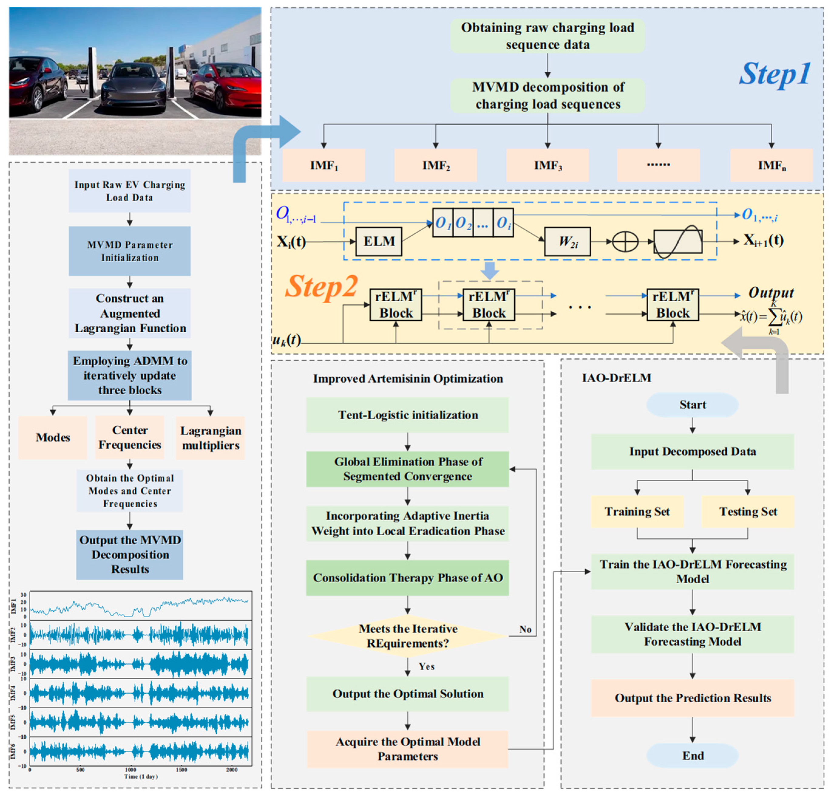
This article proposes MVMD-IAO-DrELM, a hybrid deep learning prediction model for EV charging load prediction. This paper first decomposes and processes charging load data using MVMD and then uses the IAO to enhance the accuracy of the DrELM prediction model. The IAO algorithm improves the predictive performance of the model by optimizing the hyperparameters of the DrELM prediction model.

The overall procedure flow of the model can be summarized as follows:

Step 1. The MVMD decomposes the original load data into $K$ modal components, effectively removing noise while preserving critical information.

Step 2. The dataset is divided. For model training and validation, the dataset is divided into a training set and a test set in a 7:3 proportion.

Step 3. The DrELM prediction model is trained.

Step 4. The hyperparameters (number of hidden nodes $L$, number of model layers $z$, and feature fusion weight parameter $\chi$) of the DrELM prediction model are optimized using the improved artemisinin (IAO) optimization algorithm.

Step 5. The trained IAO-DrELM model takes each decomposed component $u_k(t)$ as input and outputs its predicted value ${\widehat{u}}_k(t)$.

Step 6. A linear summation of all forecast results is performed to derive the final charging load forecast outcome.

$$\widehat{x}(t)={\displaystyle \sum _{k=1}^K{\widehat{u}}_k(t)}$$

(21)

where $\widehat{x}(t)$ denotes the total predicted value obtained from the final reconstruction.

The flowchart of the proposed MVMD-IAO-DrELM hybrid deep learning prediction model is shown in Figure 2.

4. Case Study

4.1. Data Sources

To verify the stability and effectiveness of the proposed MVMD-IAO-DrELM hybrid deep learning prediction model, three publicly available datasets from different regions were used: ShenZhen (https://opendata.sz.gov.cn/), Perth (https://data.pkc.gov.uk/), and EvnetNL (https://www.elaad.nl).

The Shenzhen dataset consists of data on EV charging stations at a ground-level car park in Bao’an District, Shenzhen City, Guangdong Province, with coordinates (22.726478°, 113.849316°). The dataset covers the period from 1 January 2019 to 1 August 2020, with a sampling interval of 1 h. This article selected spring load data from 1 January 2019 to 31 March 2019, comprising a total of 2160 hourly records. Each record primarily contains the timestamp and the charging load (e.g., in kW or kWh).

The Perth dataset consists of anonymized records from 41 EV charging points under the Scottish Tolling Scheme. The dataset spans the period from January 2017 to December 2019, with a sampling interval of one hour. This article selected data from May 2018 to August 2018, with a total of 2621 records, each record containing 10 different data points.

The EVnetNL dataset provides anonymized records of EV charging points for ElaadNL. The dataset selected for this article covers the period from September 2019 to December 2019, with a sampling interval of one hour, comprising a total of 2620 records, each of which contain 11 different data points.

4.2. Data Processing

The original dataset contains a large amount of charging information, but it also includes outliers and missing values. These cannot be used directly for model training and prediction. In order to meet the experimental requirements, the original EV charging load data must be preprocessed and converted into a time-series format suitable for model input.

For a small amount of missing data, linear interpolation was employed to fill in the gaps. For extended consecutive gaps, the entire affected time segments were removed. The paper also employs a statistical method based on the interquartile range to identify outliers, treating data points falling outside this range as outliers. Rather than deleting these outliers, they were smoothly replaced with the average of their adjacent normal points to maintain time-series continuity. Before inputting data into the model, normalize the data. The paper employs Min-Max normalization to linearly scale all data within the interval $[0,1]$. Data normalization prevents certain data features from dominating model training due to differing units, thereby enhancing the convergence speed and stability of the model.

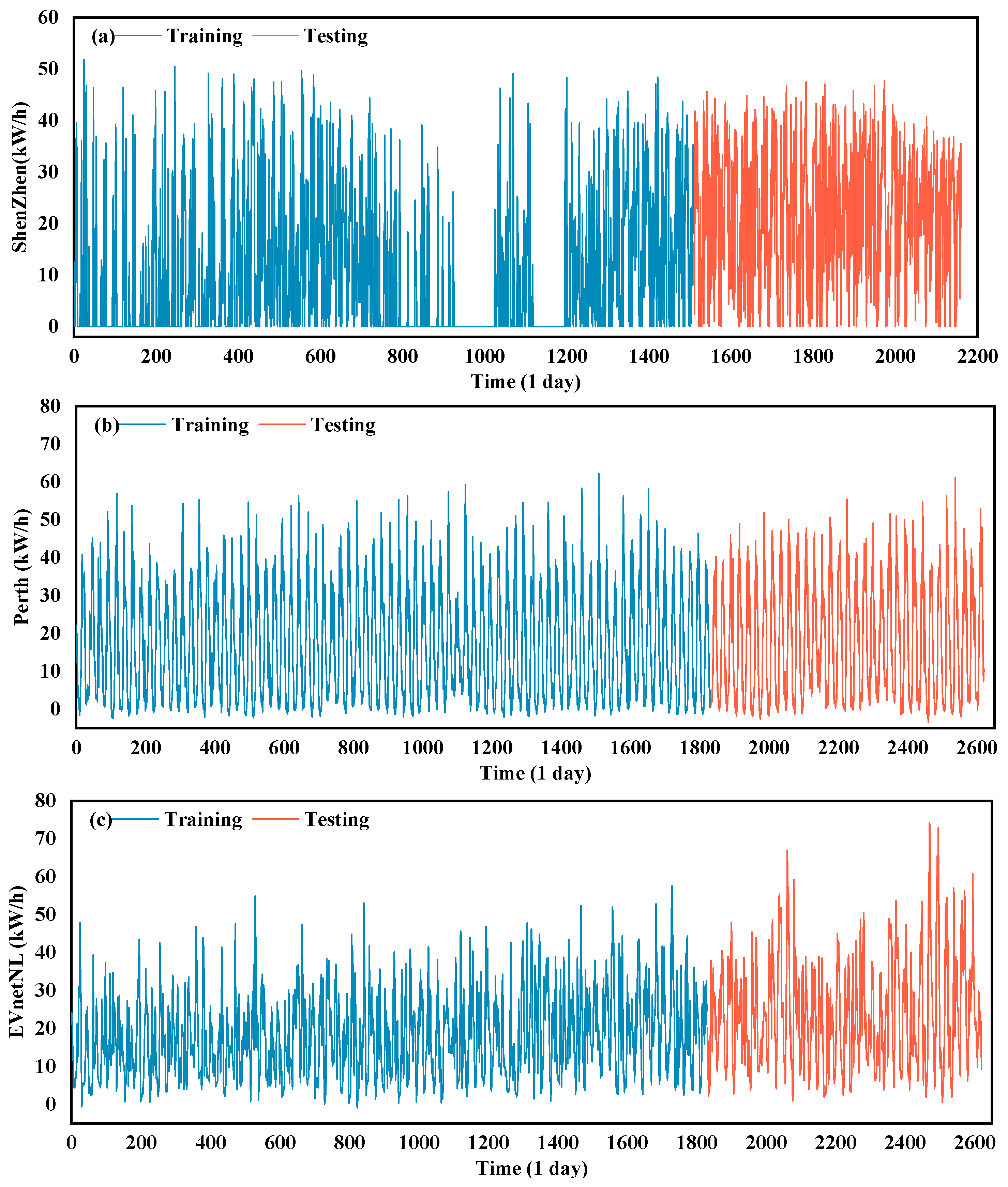
Following the preprocessing of the data, the charging load datasets for the three regions contained 2160, 2621, and 2620 transaction records, respectively. The datasets from these three regions were split into training and test sets in a ratio of 7:3. The first 70% of the data is used to train the model. The remaining 30% is used to test and validate the model. Figure 3 shows the information of the divided dataset.

4.3. MVMD Decomposition

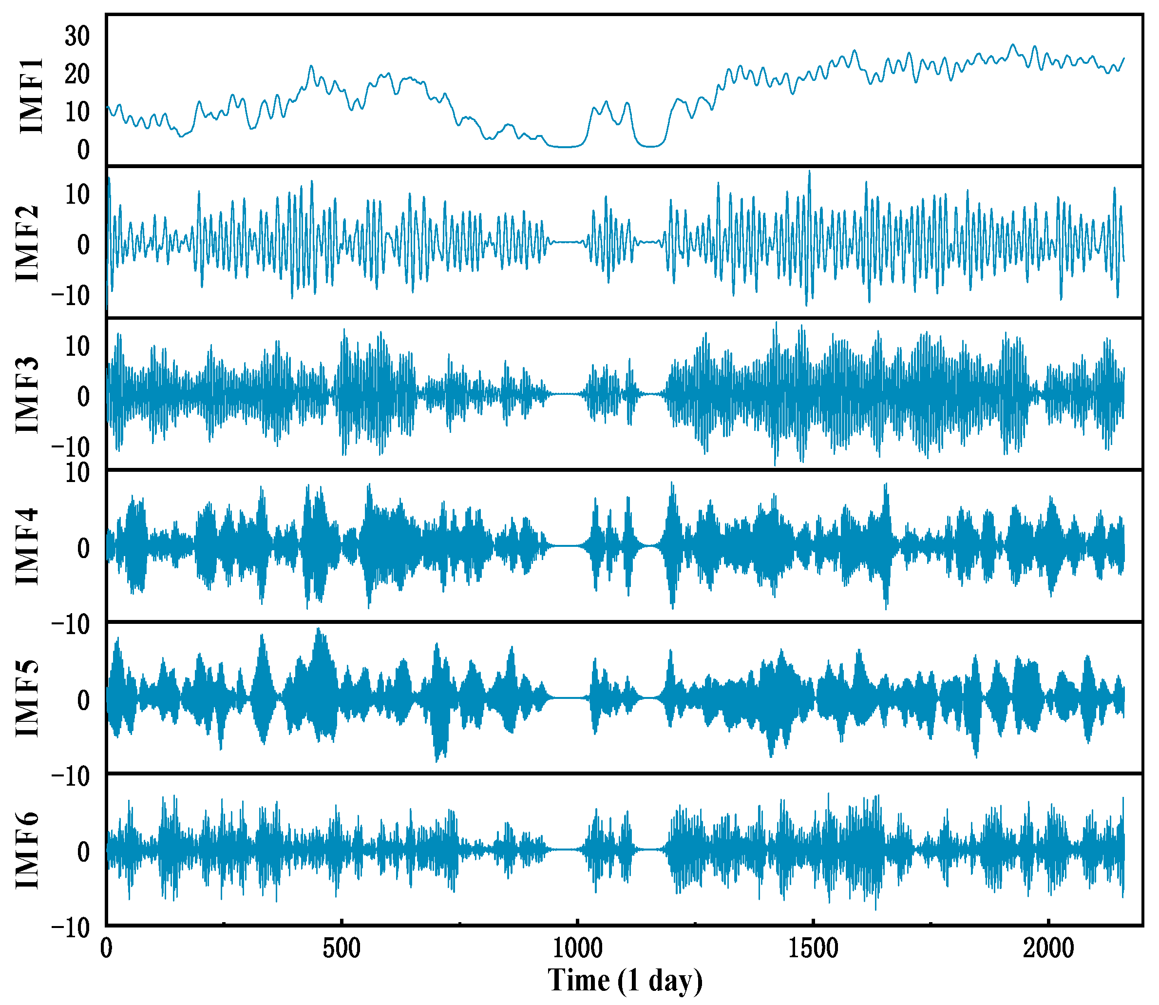
The MVMD method is used to decompose EV charging load data into multiple intrinsic modal function (IMF) components, as shown by the Shenzhen dataset. MVMD controls the fineness of decomposition by introducing a penalty term from variational methods. The quality of the decomposition results and the number of components can be controlled by adjusting the hyperparameters. The load component is decomposed within the raw data into multiple relevant components, including instantaneous rates of change encompassing the load, short-term trends of the load, and time-series characteristics strongly correlated with load periodicity, thereby enhancing the predictive accuracy of charging load sequences.

The penalty term weight alpha parameter is set to 2000; the number of modes is set to 6, and the convergence tolerance is set to 1 × 10⁻⁷ [29]. And the MVMD decomposition results of the Shenzhen charging load signal are shown in Figure 4.

4.4. Model Performance Evaluation Metrics

This article primarily uses four performance metrics to measure model accuracy, including Mean Squared Error (MSE), Mean Absolute Error (MAE), Root Mean Squared Error (RMSE), and Coefficient of Determination (R²). MSE is the Mean Squared Error, which is the average of the squared differences between the predicted and actual values. MAE is the Mean Absolute Error, which is the average of the absolute differences between the predicted and actual values. RMSE is the Root Mean Squared Error, which is the square root of the MSE. The Coefficient of Determination R² is used to measure the goodness of fit of a model. If its value is close to 1, the model fits well; if it is close to 0, the fit is poor.

The following formula is used to calculate the evaluation index:

$$\mathrm{MSE}={\displaystyle \frac{1}{Total}}{\displaystyle \sum _{i=1}^{Total}{(Y_{actual,i}-{\widehat{Y}}_{predictive,i})}^2}$$

(22)

$$\mathrm{MAE}={\displaystyle \frac{1}{Toal}}{\displaystyle \sum _{i=1}^{Toal}\left|Y_{actual,i}-{\widehat{Y}}_{predictive,i}\right|}$$

(23)

$$\mathrm{RMSE}=\sqrt{{\displaystyle \frac{1}{Toal}}{\displaystyle \sum _{i=1}^{Toal}{(Y_{actual,i}-{\widehat{Y}}_{predictive,i})}^2}}$$

(24)

$${\mathrm{R}}^2=1-{\displaystyle \frac{{\displaystyle \sum _{i=1}^{Toal}{({\widehat{Y}}_{predictive,i}-Y_{actual,i})}^2}}{{\displaystyle \sum _{i=1}^{Toal}{({\overline{Y}}_{actual,i}-Y_{actual,i})}^2}}}$$

(25)

where $Toal$ denotes the total number of sample data; $Y_{actual,i}$ denotes the true value; ${\overline{Y}}_{actual,i}$ denotes the average value of the true value; ${\widehat{Y}}_{predictive,i}$ denotes the predicted value.

5. Experimental Results and Discussion

5.1. Performance Comparison Between the DrELM and Sequential Models

To validate the appropriateness of the proposed hybrid model MVMD-IAO-DrELM, the paper conducts comparative experiments against multiple benchmark models using the ShenZhen dataset. These include traditional single models (BP, LSTM, ELM, GRU, Transformer, DrELM) as well as hybrid models incorporating signal decomposition (EMD-DrELM, VMD-DrELM, MVMD-DrELM). The performance metrics of each model on the test set are shown in

Table 1. Performance comparison of different models.

Models	MSE	RMSE	MAE	R2 (%)
BP	33.2369	5.7651	4.5577	82.52%
LSTM	27.1997	5.2153	4.1614	85.87%
ELM	26.5322	5.1509	4.0213	86.05%
GRU	26.9878	5.1950	4.0671	85.91%
Transformer	24.5070	4.9505	3.9446	87.14%
DrELM	20.1206	4.4856	3.6319	89.43%
EMD-DrELM	18.0196	4.2449	3.3955	90.54%
VMD-DrELM	17.5789	4.1927	3.3212	90.76%
MVMD-DrELM	15.6927	3.9614	3.1604	91.79%

.

Through an analysis of the results presented in Table 1, the following conclusions may be drawn:

(1)

Within a single model framework, the DrELM outperforms BP, LSTM, ELM, GRU, and Transformer across all four metrics: MSE, RMSE, MAE, and R². Compared with the baseline ELM model, the DrELM reduces the MSE, RMSE, and MAE by 24.17%, 12.92%, and 9.68%, respectively, while increasing R² to 89.43%. The results demonstrate that the DrELM has stronger nonlinear fitting and generalization capabilities when handling complex time series. It also explains why the DrELM model was selected as the core predictor.

(2)

Following the introduction of signal decomposition techniques, all decomposition-based hybrid models (EMD/VMD/MVMD-DrELM) significantly outperformed the standalone DrELM model. Compared with the DrELM, the MVMD-DrELM achieved reductions in MSE, RMSE, and MAE of 22.01%, 11.69%, and 12.98%, respectively, whilst the R² value increased to 91.79%. The results demonstrate that decomposing the original signal into multiple, relatively stationary sub-modes effectively mitigates the interference posed by sequence non-stationarity to the prediction model.

(3)

All error metrics for the MVMD-DrELM outperform those of the VMD-DrELM and the EMD-DrELM. Compared with the VMD-DrELM, its MSE, RMSE, and MAE were further reduced by 10.73%, 5.52%, and 4.84%, respectively. The results further validate the superiority of MVMD in processing multivariate signals, avoiding modal aliasing and information loss. The model reconstructs the final load sequence by linearly weighting and summing the predictions of each modal component. Experimental results demonstrate that this strategy maintains prediction consistency without introducing significant reconstruction error, further validating the feasibility and stability of the proposed framework.

5.2. Analysis of the MVMD-IAO-DrELM Model Prediction Results

In order to validate the effectiveness of the proposed MVMD-IAO-DrELM hybrid model in predicting EV charging loads, this paper compares its results with those of eight other models on the Shenzhen dataset. The eight models in the study are as follows: single models CNN, LSSVM, ELM, Regularized Extreme Learning Machine (RELM), DrELM and combination prediction models VMD-DrELM, MVMD-DrELM, and MVMD-AO-DrELM. This paper evaluates the test results of the prediction model using four common metrics: MSE, RMSE, MAE, and R².

Table 2. Comparison of load forecasting results for the ShenZhen dataset.

Models	MSE	RMSE	MAE	R2 (%)
CNN	32.8351	5.7302	4.6190	83.57%
LSSVM	29.5549	5.4364	4.3112	85.02%
ELM	26.5322	5.1509	4.0213	86.05%
RELM	23.0818	4.8044	3.8071	87.93%
DrELM	20.1206	4.4856	3.6319	89.43%
VMD-DrELM	17.5789	4.1927	3.3212	90.76%
MVMD-DrELM	15.6927	3.9614	3.1604	91.79%
MVMD-AO-DrELM	14.5710	3.8172	3.0494	92.35%
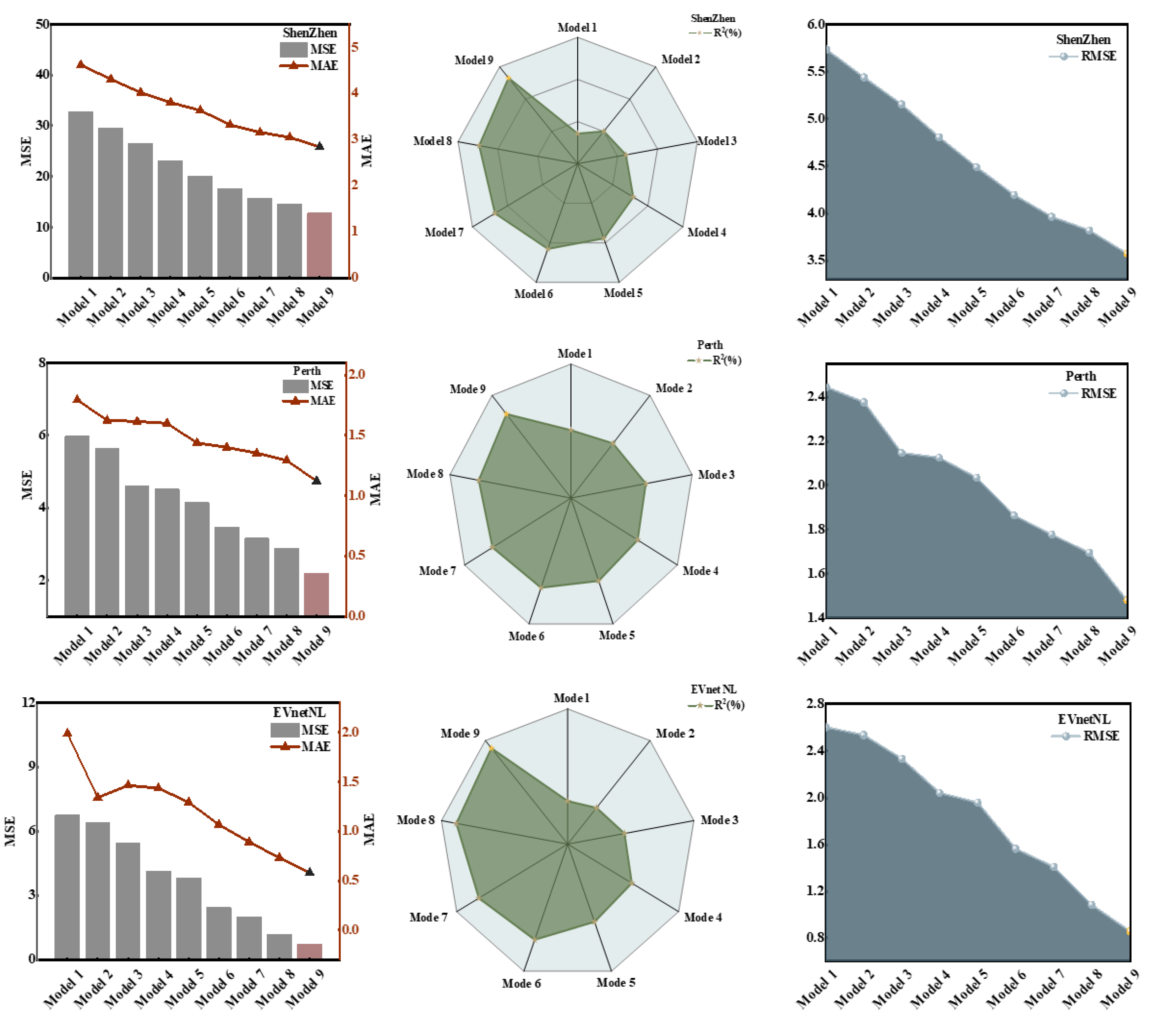
MVMD-IAO-DrELM	12.7700	3.5735	2.8405	93.29%

shows the four error metrics of the ShenZhen dataset after prediction using the above nine models. Furthermore, to more intuitively demonstrate the error metrics of each model on the ShenZhen dataset, this paper uses dual-Y-axis column-dot charts, line charts, and radar charts for display, as shown in Figure 5. At the same time, in order to present the graphics in a more convenient and intuitive manner, each model name is replaced with Model 1 to Model 9, as shown in

Table 3. Model abbreviations and corresponding algorithms.

Name	Models
Model 1	CNN
Model 2	LSSVM
Model 3	ELM
Model 4	RELM
Model 5	DrELM
Model 6	VMD-DrELM
Model 7	MVMD-DrELM
Model 8	MVMD-AO-DrELM
Model 9	MVMD-IAO-DrELM

.

The following conclusions can be drawn through a careful analysis of Table 2 and Figure 5:

(1)

After comparing the proposed hybrid deep learning prediction model MVMD-IAO-DrELM with eight other models, the error metric results show that this model has the most accurate prediction results. The predictive model proposed in this paper performed as follows in terms of the four error metrics: the MSE value was 12.7700; the RMSE value was 3.5735; the MAE value was 2.8405; and the R² value was 93.29%.

(2)

The DrELM model is a bit better than the other single models: CNN, LSSVM, ELM, and RELM. Compared with the basic ELM model, the DrELM achieved reductions in MSE, RMSE, and MAE of 24.17%, 12.92%, and 9.68%, respectively.

(3)

During model training on the Shenzhen dataset, the MSE, RMSE, and MAE values of the MVMD-DrELM were 15.6927, 3.9614, and 3.1604, respectively. These values were reduced by 22.01%, 11.69%, and 12.98%, respectively, compared with the DrELM single model.

(4)

In the experiment, this paper also used VMD signal decomposition and MVMD signal decomposition for comparison. The experimental results show that the signal decomposition effect of MVMD is slightly better than that of VMD, with the error indicators MSE, RMSE, and MAE decreasing by 10.73%, 5.52%, and 4.84%, respectively.

(5)

The MVMD-AO-DrELM showed a 7.15% reduction in MSE, a 3.64% reduction in RMSE, and a 3.51% reduction in MAE when compared with the experimental results of the MVMD-DrELM. The experimental results show that the AO algorithm can optimize the parameters of the DrELM model, improving its efficiency and accuracy.

(6)

Compared with the MVMD-AO-DrELM model, the MVMD-IAO-DrELM model proposed in this paper exhibits lower error metrics (MSE, RMSE, and MAE) and a higher R² Coefficient of Determination. The experimental results demonstrate the positive impact of the improved IAO algorithm on the prediction model parameter optimization.

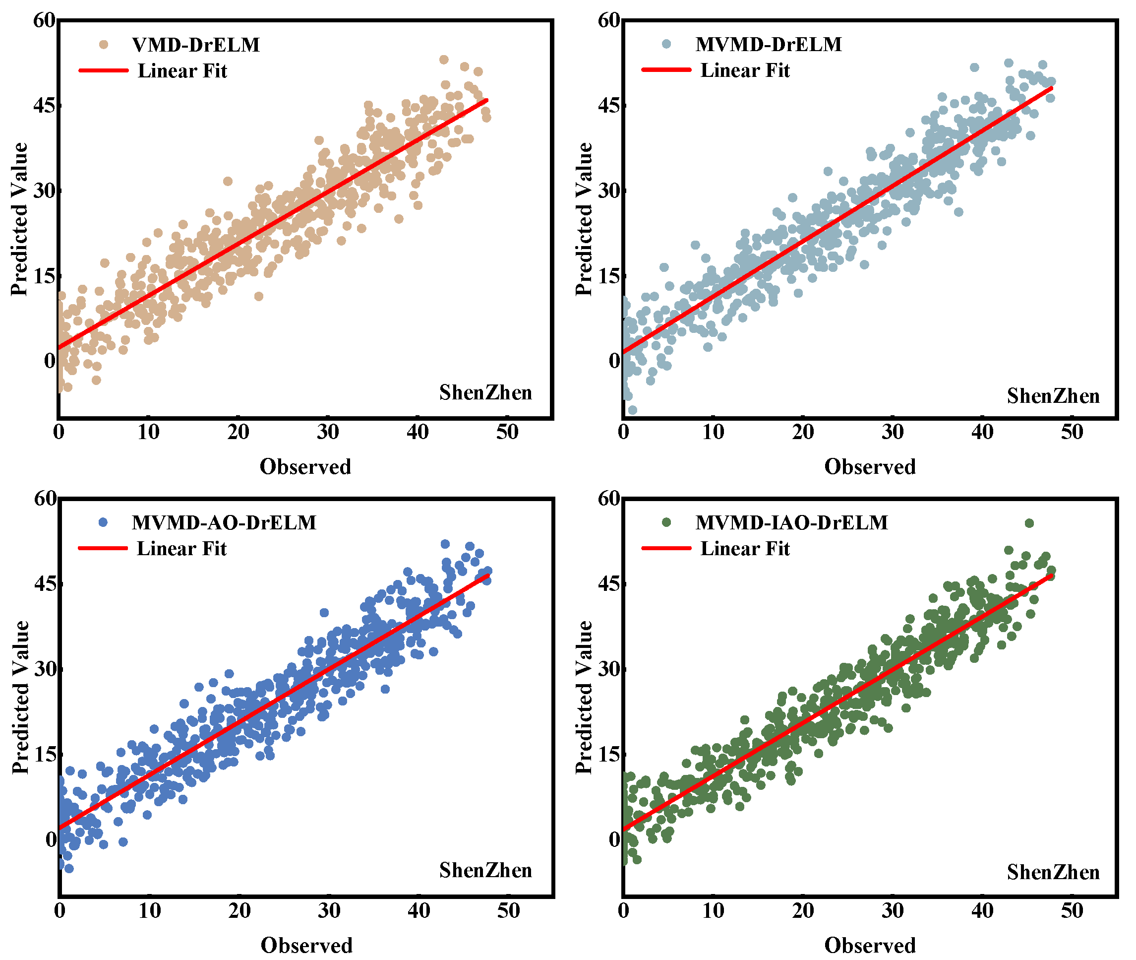
Figure 6 shows the experimental results of the four prediction models, VMD-DrELM, MVMD-DrELM, MVMD-AO-DrELM, and MVMD-IAO-DrELM, on the ShenZhen dataset. As Figure 6 shows, the MVMD-IAO-DrELM prediction model proposed in this paper has the best fitting effect. The analysis above indicates that the MVMD-IAO-DrELM prediction model is a more suitable option for EV charging load data, resulting in more-precise prediction outcomes.

5.3. Combinatorial Predictive Model Generalization Ability Test

To fully validate the model’s generalization ability beyond a single region, this paper evaluates the hybrid deep prediction model using multi-regional charging load data: the Perth and EVnetNL datasets.

Table 4. Comparison of load forecasting results for the Perth dataset.

Models	MSE	RMSE	MAE	R2 (%)
CNN	5.9688	2.4431	1.7932	97.53%
LSSVM	5.6400	2.3749	1.6236	97.66%
ELM	4.6047	2.1458	1.6157	98.09%
RELM	4.5140	2.1246	1.5995	98.13%
DrELM	4.1381	2.0342	1.4372	98.29%
VMD-DrELM	3.4728	1.8635	1.4006	98.56%
MVMD-DrELM	3.1582	1.7771	1.3523	98.69%
MVMD-AO-DrELM	2.8724	1.6948	1.2919	98.81%
MVMD-IAO-DrELM	2.1917	1.4805	1.1209	99.09%

shows the experimental error metric results for the Perth dataset, while

Table 5. Comparison of load forecasting results for the EVnetNL dataset.

Models	MSE	RMSE	MAE	R2 (%)
CNN	6.7531	2.5987	1.9900	96.59%
LSSVM	6.4075	2.5313	1.3411	96.75%
ELM	5.4273	2.3296	1.4646	97.25%
RELM	4.1482	2.0367	1.4381	97.89%
DrELM	3.8171	1.9538	1.2935	98.06%
VMD-DrELM	2.4338	1.5601	1.0671	98.76%
MVMD-DrELM	1.9749	1.4053	0.8919	99.00%
MVMD-AO-DrELM	1.1682	1.0808	0.7311	99.41%
MVMD-IAO-DrELM	0.7346	0.8571	0.5801	99.63%

shows the results for the EVnetNL dataset. To demonstrate the performance of the MVMD-IAO-DrELM hybrid deep prediction model on these two datasets more intuitively, the experimental results of each prediction model are presented in Figure 5.

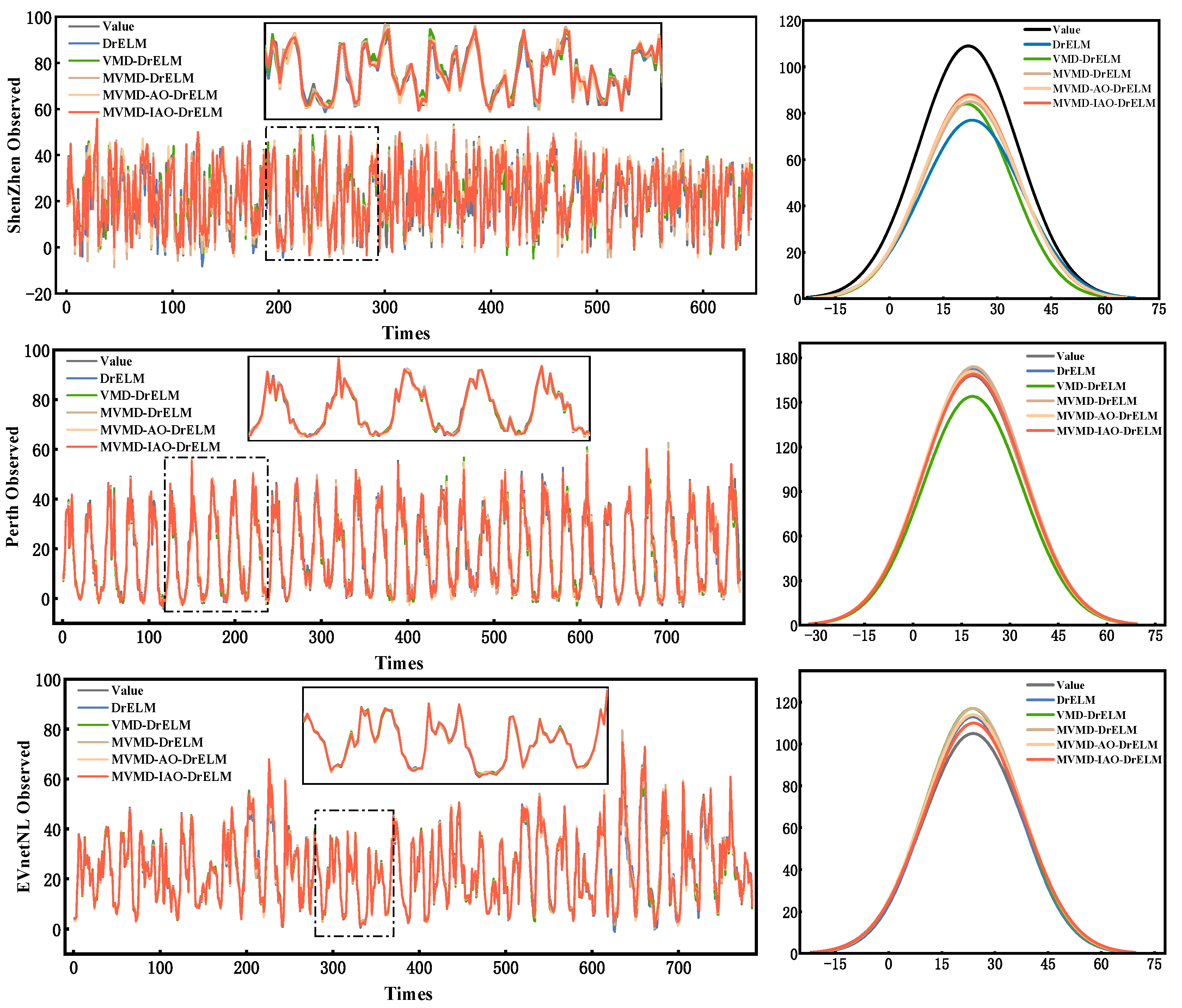
As shown in Table 4 and Table 5, the proposed hybrid deep learning prediction model MVMD-IAO-DrELM performs very well on the Perth and EVnetNL datasets. On the Perth dataset, the MSE, RMSE, MAE, and R² values of the proposed hybrid deep prediction model were 2.1917, 1.4805, 1.1209, and 99.09%, respectively. Compared with the single model prediction DrELM, the MSE decreased by 47.04%: the RMSE decreased by 27.22%; and the MAE decreased by 22%. On the EVnetNL dataset, the MSE, RMSE, MAE, and R² of the proposed hybrid deep prediction model achieved 0.7346, 0.8571, 0.5801, and 99.63%, respectively. Compared with the single model prediction DrELM, the MSE decreased by 80.76%; the RMSE decreased by 56.13%; the MAE decreased by 55.15%. As can be clearly seen from Figure 5, there is a significant improvement in the evaluation indicators of the MVMD-IAO-DrELM prediction model compared with those for other prediction models. Figure 6 provides further illustration of the linear fit and error normal distribution of the hybrid deep prediction model proposed in this paper on the Perth and EVnetNL datasets.

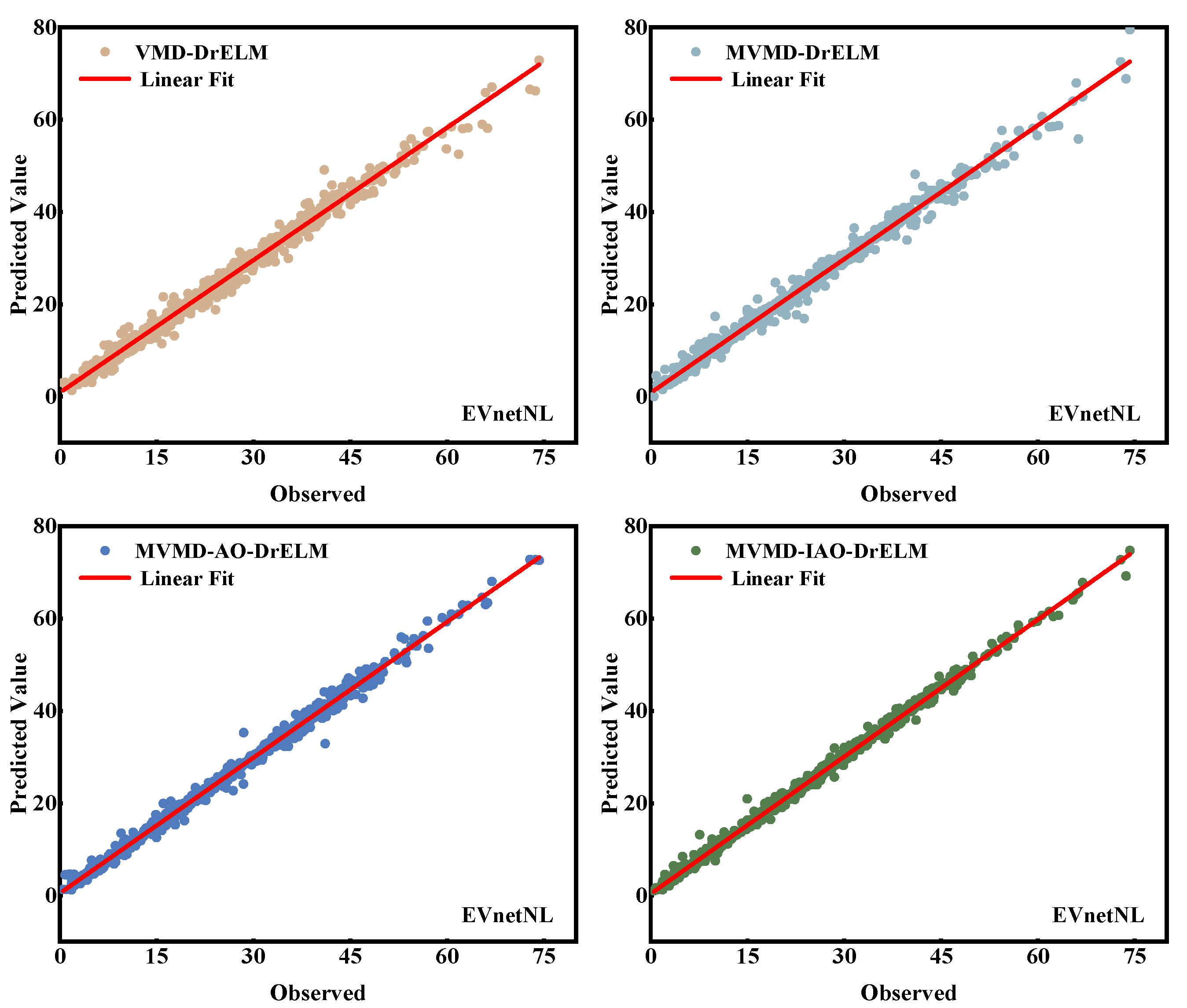
Figure 7 shows that the prediction results of the model remain optimal after incorporating the MVMD signal decomposition technique. This also proves the effectiveness of the prediction model proposed in this paper, suggesting that the accuracy of the prediction model can be further improved by using MVMD signal decomposition technology. The error distribution diagram in Figure 7 shows that the MVMD-IAO-DrELM prediction model has the narrowest prediction bandwidth and normal distribution in the Perth and EVnetNL datasets. The experimental results of these two datasets further prove that the prediction performance of the hybrid deep prediction model proposed in this paper is optimal. Figure 8 and Figure 9 continue to plot the experimental results for the four prediction models (VMD-DrELM, MVMD-DrELM, MVMD-AO-DrELM, and MVMD-IAO-DrELM) on the Perth and EVnetNL datasets.

It is clear from Figure 8 and Figure 9 that the MVMD-IAO-DrELM prediction model proposed still provides the best fit. The above analysis further demonstrates that the MVMD-IAO-DrELM prediction model is effective in predicting EV charging loads and can produce more-accurate results.

6. Conclusions

This paper proposes a hybrid deep learning prediction model based on MVMD-IAO-DrELM. Across all datasets, the proposed model achieved the lowest error in MSE, RMSE, and MAE, and the highest R² value. And it achieved RMSE values of 3.57, 1.48, and 0.86 for the ShenZhen, Perth, and EVnetNL datasets, respectively. Compared with traditional single models like CNN, LSSVM, and ELM, it reduced RMSE and MAE by approximately 48% and 49% on average, while improving R² by 1.6%. Compared with the previously proposed MVMD-AO-DrELM hybrid model, this model achieved a reduction of approximately 13% in both RMSE and MAE. Consequently, the MVMD-IAO-DrELM model presented demonstrates superior predictive performance in forecasting EV charging loads.

Although the model proposed in this paper demonstrates superior predictive accuracy compared with other traditional forecasting models, it nevertheless exhibits certain limitations. Firstly, the predictive performance of the model relies on high-quality multidimensional historical data. Should the data exhibit significant missing values, noise, or other issues, the prediction accuracy of the model may be compromised. Secondly, although the model demonstrates sound predictive capabilities on datasets from ShenZhen, Perth, and EVnetNL, its predictive performance in other regions or at other charging stations remains unclear. Moreover, this model is primarily constructed based on load time-series data and does not incorporate external variables such as weather, public holidays, or traffic flow. Consequently, its applicability in complex scenarios may be limited. And the study primarily focuses on forecasting the total load volume and does not delve into the specific impact of harmonic distortion introduced by charging behavior on the power quality of the grid. Moreover, the extreme intermittency of load remains an inherent challenge for all forecasting models. Although this model can smooth the forecast curve to some extent, it cannot fundamentally eliminate its randomness.

Accordingly, future work will focus on the following:

(1)

Prioritizing improving the accuracy and reliability of the model when dealing with situations involving missing data and noise interference.

(2)

Investigating how trained models can adapt quickly to new regions or charging station types with minimal additional training, thereby improving their generalization capabilities and practical utility.

(3)

Strengthening the spatiotemporal feature extraction capabilities of the model by integrating external conditions such as weather, public holidays, and traffic volume.

(4)

Considering integrating the model with the energy management systems to optimize the coordinated operation between EVs and the power grid holistically.

In summary, the hybrid deep learning prediction model proposed in this paper effectively uses the signal decomposition capability of MVMD, the prediction efficiency of DrELM, and the parameter optimization prowess of the IAO algorithm. It offers a novel and practical solution for EV charging load forecasting, holding significant potential for real-world application in the evolving smart grid landscape.

References

1. Global EV Outlook 2024: Moving Towards Increased Affordability; International Energy Agency: Paris, France, 2024; Available online: https://www.iea.org/reports/global-ev-outlook-2024 (accessed on 15 March 2025).
2. Liu, Y.S.; Tayarani, M.; Gao, H.O. An activity-based travel and charging behavior model for simulating battery electric vehicle charging demand. Energy 2022, 258, 124938. [Google Scholar] [CrossRef]
3. Xia, F.; Chen, H.; Yan, M.; Gan, W.; Zhou, Q.; Ding, T.; Wang, X.; Wang, L.; Chen, L. Market-Based Coordinated Planning of Fast Charging Station and Dynamic Wireless Charging System Considering Energy Demand Assignment. IEEE Trans. Smart Grid 2023, 15, 1913–1925. [Google Scholar] [CrossRef]
4. Siddiqui, J.; Ahmed, U.; Amin, A.; Alharbi, T.; Alharbi, A.; Aziz, I.; Khan, A.R.; Mahmood, A. Electric Vehicle charging station load forecasting with an integrated DeepBoost ap-proach. Alex. Eng. J. 2025, 116, 331–341. [Google Scholar] [CrossRef]
5. Palou, J.T.V.; González, J.S.; Santos, J.M.R.; Fernández, J.M.R. A novel weight-based ensemble method for emerging energy players: An application to electric vehicle load prediction. Energy AI 2025, 20, 100510. [Google Scholar] [CrossRef]
6. Akil, M.; Dokur, E.; Bayindir, R. Analysis of Electric Vehicle Charging Demand Forecasting Model based on Monte Carlo Simulation and EMD-BO-LSTM. In Proceedings of the 2022 10th International Conference on Smart Grid (icSmartGrid), Istanbul, Turkey, 27–29 June 2022; pp. 356–362. [Google Scholar]
7. Akinola, I.T.; Sun, Y.; Adebayo, I.G.; Wang, Z. Daily peak demand forecasting using Pelican Algorithm optimised Support Vector Machine (POA-SVM). Energy Rep. 2024, 12, 4438–4448. [Google Scholar] [CrossRef]
8. Yaghoubi, E.; Khamees, A.; Razmi, D.; Lu, T. A systematic review and meta-analysis of machine learning, deep learning, and ensemble learning approaches in predicting EV charging behavior. Eng. Appl. Artif. Intell. 2024, 135, 108789. [Google Scholar] [CrossRef]
9. Jiang, P.; Li, R.; Liu, N.; Gao, Y. A novel composite electricity demand forecasting framework by data processing and optimized support vector machine. Appl. Energy 2020, 260, 114243. [Google Scholar] [CrossRef]
10. Pesantez, E.J.; Li, B.; Lee, C.; Zhao, Z.; Butala, M.; Stillwell, A.S. A Comparison Study of Predictive Models for Electricity Demand in a Diverse Urban Environment. Energy 2023, 283, 129142. [Google Scholar] [CrossRef]
11. Sarkin Adar, Z.M.; Alhayd, A.; Todeschini, G. Predicting EV Charging Duration Using Machine Learning and Charging Transactions at Three Sites. In Proceedings of the 2024 IEEE International Conference on Industrial Technology (ICIT), Bristol, UK, 25–27 March 2024; pp. 1–6. [Google Scholar]
12. Ren, X.; Zhang, F.; Zhu, H.; Liu, Y. Quad-kernel deep convolutional neural network for intra-hour photovoltaic power forecasting. Appl. Energy 2022, 323, 119682. [Google Scholar] [CrossRef]
13. Danish, M.U.; Grolinger, K. Kolmogorov–Arnold recurrent network for short term load forecasting across diverse consumers. Energy Rep. 2025, 13, 713–727. [Google Scholar] [CrossRef]
14. Wang, S.; Zhuge, C.; Shao, C.; Wang, P.; Yang, X.; Wang, S. Short-term electric vehicle charging demand prediction: A deep learning approach. Appl. Energy 2023, 340, 121032. [Google Scholar] [CrossRef]
15. Zhao, Y.; Wang, Z.; Shen, Z.-J.M.; Sun, F. Data-driven framework for large-scale prediction of charging energy in electric vehicles. Appl. Energy 2021, 282, 116175. [Google Scholar] [CrossRef]
16. Yue, W.; Liu, Q.; Ruan, Y.; Qian, F.; Meng, H. A prediction approach with mode decomposition-recombination technique for short-term load forecasting. Sustain. Cities Soc. 2022, 85, 104034. [Google Scholar] [CrossRef]
17. Guo, H.; Chen, L.; Wang, Z.; Li, L. Day-ahead prediction of electric vehicle charging demand based on quadratic decomposition and dual attention mechanisms. Appl. Energy 2025, 381, 125198. [Google Scholar] [CrossRef]
18. Zhang, X.; Kong, X.; Yan, R.; Liu, Y.; Xia, P.; Sun, X.; Zeng, R.; Li, H. Data-driven cooling, heating and electrical load prediction for building integrated with electric vehicles considering occupant travel behavior. Energy 2023, 264, 126274. [Google Scholar] [CrossRef]
19. Zhao, Z.; Zhang, Y.; Yang, Y.; Yuan, S. Load forecasting via Grey Model-Least Squares Support Vector Machine model and spatial-temporal distribution of electric consumption intensity. Energy 2022, 255, 124468. [Google Scholar] [CrossRef]
20. Kim, H.J.; Kim, M.K. Spatial-Temporal Graph Convolutional-Based Recurrent Network for Electric Vehicle Charging Stations Demand Forecasting in Energy Market. IEEE Trans. Smart Grid 2024, 15, 3979–3993. [Google Scholar] [CrossRef]
21. Yin, W.; Ji, J.; Wen, T.; Zhang, C. Study on orderly charging strategy of EV with load forecasting. Energy 2023, 278, 127818. [Google Scholar] [CrossRef]
22. Rehman, N.U.; Aftab, H. Multivariate Variational Mode Decomposition. IEEE Trans. Signal Process. 2019, 67, 6039–6052. [Google Scholar] [CrossRef]
23. Rilling, G.; Flandrin, P. One or Two Frequencies? The Empirical Mode Decomposition Answers. IEEE Trans. Signal Process. 2007, 56, 85–95. [Google Scholar] [CrossRef]
24. Dragomiretskiy, K.; Zosso, D. Variational mode decomposition. IEEE Trans. Signal Process. 2013, 62, 531–544. [Google Scholar] [CrossRef]
25. Zeng, H.; Wu, B.; Fang, H.; Lin, J. Interpretable wind speed forecasting through two-stage decomposition with comprehensive relative importance analysis. Appl. Energy 2025, 392, 126015. [Google Scholar] [CrossRef]
26. Yuan, C.; Zhao, D.; Heidari, A.A.; Liu, L.; Chen, Y.; Wu, Z.; Chen, H. Artemisinin optimization based on malaria therapy: Algorithm and applications to medical image segmentation. Displays 2024, 84, 102740. [Google Scholar] [CrossRef]
27. Yu, W.; Zhuang, F.; He, Q.; Shi, Z. Learning deep representations via extreme learning machines. Neurocomputing 2015, 149, 308–315. [Google Scholar] [CrossRef]
28. Huang, G.B.; Zhu, Q.Y.; Siew, C.K. Extreme learning machine: A new learning scheme of feedforward neural networks. Neurocomputing 2004, 2, 985–990. [Google Scholar]
29. Wang, J.; Chen, Q.; Lang, X.; Liu, S.; Liu, Y.; Su, H. A modified multivariate variational mode decomposition for multi-channel signal processing. In Proceedings of the 2023 8th International Conference on Communication, Image and Signal Processing (CCISP), Chengdu, China, 17–19 November 2023; pp. 384–390. [Google Scholar]
Figure 1. Structure of the DrELM model.
Energies 18 06061 g001
Figure 2. Flowchart of the proposed MVMD-IAO-DrELM hybrid deep learning model.
Energies 18 06061 g002
Figure 3. Division of the Electric Vehicle Charging Station (EVCS) datasets: (a) ShenZhen; (b) Perth; (c) EVnetNL.
Energies 18 06061 g003
Figure 4. MVMD decomposition results of the Shenzhen charging load signal (K = 6).
Energies 18 06061 g004
Figure 5. Comparison of MSE, MAE, RMSE, and R2 results for ShenZhen, Perth, and EVnetNL datasets. (The red highlighting is used to emphasize the MSE of the proposed model, underscoring its performance difference from other baseline methods).
Energies 18 06061 g005
Figure 6. Linear fit plot for the ShenZhen dataset.
Energies 18 06061 g006
Figure 7. The linear fit and error normal distribution plots of the combined prediction model for the ShenZhen, Perth, and EVnetNL datasets.
Energies 18 06061 g007
Figure 8. Linear fit plot for the Perth dataset.
Energies 18 06061 g008
Figure 9. Linear fit plot for the EVnetNL dataset.
Energies 18 06061 g009