Abstract
The transition from conventional fossil-fueled buses to electric buses (EBs) is accelerating in the global public transportation sector. However, owing to the limitations of battery lifespan and capacity, EBs have a shorter driving range than conventional buses, and their power consumption is highly variable depending on the ambient temperature. In addition, battery lifespans are affected by charging and discharging cycles and battery age over time in all situations, which requires a method of operation that considers these factors. In this study, we estimated the driving, heating, and cooling energy consumptions based on the dispatch schedule and actual power consumption of EBs. The estimated energy consumption was then used as an input to plan the amount of charging power by time of day to optimize the charging and battery degradation costs. The optimization methodology employed mixed-integer linear programming (MILP), which facilitates discrete charging decision-making and ensures an optimum solution for operation costs by taking cost factors into account. In this phase, the scenarios were configured according to the time-of-use (TOU) charging cost and whether or not battery degradation. Battery degradation can be divided into cycle and calendar aging. The scenarios that considered both TOU and battery degradation reduced the average operating costs by approximately 1.43, 12.3, and 5.69% in spring/fall, summer, and winter, respectively, compared with scenarios that did not consider either.
1. Introduction
CO2 emissions from the transportation sector grew at an average annual rate of 1.7% from 1990 to 2022, and by 2023, these accounted for 21.11% of total emissions [1,2]. In this context, electric buses (EBs) are emerging as promising alternatives that offer significant advantages over conventional diesel-powered buses. In addition to reducing greenhouse gas (GHG) emissions, the introduction of electric buses can help create healthier urban environments by reducing noise pollution and improving air quality. In addition to environmental benefits, EBs also offer economic benefits, such as reductions in operating costs and the promotion of technological innovation in the transportation sector [3]. Therefore, the adoption of EBs in public transportation systems is being accelerated to help achieve carbon neutrality [4,5].
Bus operations are generally performed by picking up and dropping off passengers along a fixed route, and establishing dispatching and charging schedules for EBs is considered one of the major tasks of bus operators [6,7]. EBs require frequent recharging because of their limited battery capacity, and managing the battery lifespan is an important factor for economic operation because of the high cost of batteries [8,9]. Furthermore, charging costs vary with the time of day, and charging schedule planning is essential for economical operation [10,11]. In particular, the energy consumption of EBs can increase both while driving and from additional factors, such as heating and cooling systems, which can directly limit their driving range [12,13]. Therefore, an optimized dispatching and charging strategy that accounts for these limitations is essential to ensure cost-effective EB operations [14,15].
Several studies have been conducted on EB scheduling. In [4,16,17,18,19], EB charging-scheduling algorithms were proposed. Ref. [4] proposed a dynamic programming algorithm based on the Lagrangian mitigation framework and optimized the charging schedule for 10 actual EB routes and 13 charging stations. Ref. [16] optimized the charging schedule of six circular EBs on university campuses in Brazil using a dynamic approach based on the rolling-horizon method. Ref. [17] proposed an adaptive large neighborhood search algorithm that extends the alternative-fuel vehicle scheduling problem to the electric vehicle scheduling problem. Ref. [18] proposed a battery EB-network charging optimization (BEB-NCO) model and ref. [19] proposed an improved particle swarm optimization algorithm to optimize the dispatch and charging schedule for six routes in Beijing, China. These studies focused on developing EB charging algorithms for various operating environments to reduce economic efficiency but did not consider battery degradation.
To address this limitation, various studies [8,20,21,22] have explored the impact of battery degradation due to cycle aging, with the aim of managing battery life in EBs. Ref. [8] proposed a mixed-integer linear programming (MILP)-based EB charging strategy considering cycle aging. The battery degradation cost was calculated based on the achievable cycle count depth (ACC-DOD) of the discharge curve. Ref. [20] considered the cycle aging of a battery and proposed a branch-and-price (B&P) approach, which was designed using a column generation (CG) procedure to ensure a water purification solution and optimize the charging schedule. Ref. [21] calculated the battery performance degradation cost according to the ACC-DOD curve when considering cycle aging and proposed mixed-integer nonlinear and nonconvex programming (MINL&NCP) to solve the EB charging scheduling problem. Ref. [22] modeled the battery capacity reduction owing to cycling using a natural network (NN)-based battery degradation model and proposed an MILP-based operating strategy considering the charging cost.
Based on the reviewed studies, the existing research focuses on reducing charging costs and managing battery life by considering the power consumption from driving and cycle aging of the battery, rarely considering the energy consumption associated with calendar aging and the heating and cooling systems. Heating and cooling systems, account for a significant portion of the energy consumption of EBs, second only to driving. These systems are highly influenced by weather conditions, such as ambient temperature. If this is not considered, the additional energy consumption could result in an insufficient available battery capacity, which may impact the preplanned EB dispatch and charging schedules. Such schedule adjustments under the time-of-use (TOU) pricing system can result in battery charging during higher price periods than initially planned, thereby incurring additional costs. Furthermore, it can cause the battery’s state of charge (SoC) to deviate from its stable range. In addition, EBs that provide public transportation services have cyclical power consumption and idle times because of their fixed-route driving and dispatch schedules [23,24]. However, reviewed studies on battery degradation typically neglect calendar aging and focus only on cycle aging, potentially resulting in an underestimation of battery disposal or replacement costs. Therefore, effective battery life management must account for both cycle aging, caused by repeated charging and discharging, and calendar aging, which is influenced by internal and external environmental factors, such as ambient temperature and SoC during idle periods. Consequently, the optimization of EB operation through the integration of energy consumption from driving and heating and cooling systems while considering both cycle aging and calendar aging in the context of battery degradation will achieve reductions in actual EB operating costs. Furthermore, optimization methods frequently used by existing studies (e.g., heuristics, rolling-horizon, PSO) for the problem risk settling on local or suboptimal solutions because they cannot mathematically guarantee the global optimum [16,19]. In comparison, MILP can ensure mathematically optimal and feasible solutions under linear and integer constraints, systematically exploring feasible spaces and ensuring physically and economically consistent results. Therefore, the optimization of electric bus operations to reduce operational costs requires a MILP model that guarantees the effectiveness of the global optimal solution.
This study developed an EB charging strategy to minimize charging costs and manage battery degradation. The proposed model optimizes the EB charging strategy by considering the dispatch schedule of the EBs, battery energy consumption, degradation, and charging prices. The energy consumption model of the EBs was estimated through electricity consumption according to the driving speed, and the electricity consumption of the cooling and heating systems according to the driving time and ambient temperature. In addition, a battery degradation model was designed based on an empirical model that considers the battery cell temperature, DoD, and SoC states. These models were linearized and integrated into the charging strategy and then formulated as MILP-based models. The proposed model was verified through case studies based on whether TOU and battery degradation were considered as scenarios to evaluate the EB charging and battery life management costs.
The remainder of this paper is organized as follows. Section 2 describes the environment for the proposed EB charging strategy and the resulting system configuration. This is followed by the process of estimating the EB energy consumption, degradation, and charging cost optimization in Section 3. Finally, the case study setup and the results are presented in Section 4.
2. Proposed EB Charging Strategy
The proposed EB charging strategy aims to minimize the charging costs and battery degradation. An EB departs from the depot, reaches a turn stop, and returns to the depot without an additional charge. Upon returning to the depot, the charging system plans a charging schedule based on the remaining battery SoC and the estimated power consumption for the next trip.
Figure 1 shows the proposed EB charging mechanism. The EB operator aims to minimize both the battery charging and degradation costs The objective function consists of these two costs and can be verified in the optimization box along with the constraints. Here, the charging cost is determined based on TOU load periods and costs. The charging schedule of the EBs is determined by considering the energy consumed during each EB operation and the dispatch schedule. The energy consumption of the EB is further divided into driving and cooling/heating systems. The driving energy consumption is estimated based on the average energy consumption per kilometer, considering the driving distance and time. The heating and cooling system consumptions are estimated based on the ambient temperature and driving time. The battery capacity loss owing to degradation is calculated based on the ambient temperature, battery SoC, and DoD. This is then converted into a degradation cost based on the unit price of the battery. As can be seen in Figure 1, there are four main optimization constraints. These are the battery SOC and charger technical constraints of EB, the duration of charging and the interval between the next charging, and the movement and charging of EBs after the end of operation. These are discussed in detail in Section 3.
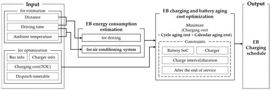
Figure 1.
EB charging system scheduling.
3. Optimization Cost of EB Charging and Battery Capacity Loss
The objective function aims to minimize the total cost, which consists of the charging cost ( and battery degradation cost (, as shown in Equation (1) where and are the EB number and set of EBs, respectively. Detailed explanations of the related variables can be found in Appendix A. and are the time and set of operation times, respectively. The charging cost () is calculated by multiplying the charging power () and TOU (), as shown in Equation (2) where is the unit conversion constant from power to energy. Equation (3) expresses the battery degradation cost (), calculated based on the battery capacity loss rate (), battery capacity of the EB (), unit cost per capacity (), end-of-life criteria (), and rate of depreciation at resale (). Here, is applied as to set the price until the end of battery life. Battery loss rate is calculated as the sum of cycle () and calendar () aging. The battery loss rate due to cycle aging () is determined by the change in battery DoD of bus between time and time during each charge and discharge cycle and parameters dependent on external temperature () and battery DoD (, ). The battery loss rate due to calendar aging is determined by the SoC of bus at time and the parameters pertaining to external temperature () and battery SoC (, ). These parameters are the seasonal external temperature parameters (, ), battery DoD and SoC states of the EB (, ), and the corresponding parameters (, , , ) were adjusted to fit the model of this study based on experimental values from the reference study [25].
The constraints on the EB SoC, charging schedule, and chargers are expressed using Equations (6)–(12). The battery SoCs at the beginning and end of the EB charging schedule are set to be the same for each EB in Equation (6). This is because a daily schedule optimization is performed; however, in reality, charging should be performed the next day. Equation (7) expresses the minimum SoC ( and maximum SoC ( constraints of the battery, whereas the SoC of EB b at time t () is calculated using Equation (8). Here, the battery SoC () of the EB at time is calculated using the battery SoC from previous timeslot, energy consumption (), charging power , unit conversion constant from power to energy , and unit conversion constant from energy to SoC . and are the charging start and end state EB. For battery life management, the minimum charging duration of the EB and the minimum waiting time between the previous charging and next charging are limited as shown in Equation (9) [26,27]. Equation (10) expresses the charging constraint after the end of the last EB operation, which determines the charging state () at time . The number of EBs that can be charged simultaneously is constrained using Equation (11) to ensure that the total number of chargers is not exceeded. Equation (12) expresses the charging power constraint. Here, is the state variable of the garaged EBs at the depot, meaning that only these EBs can be charged.
The EB energy consumption () can be expressed using Equation (13). The energy consumption due to driving () and cooling/heating systems () is calculated using Equations (14) and (15), respectively. Equation (14) expresses the energy consumption during driving () for a interval relative to the average driving speed by dividing the route distance () by the trip time of EB at the -th trip (). Here, and are parameters that have been adjusted to fit the model of this study based on the reference study [28]. Equation (15) expresses the energy consumption of the cooling/heating system () by converting the heating and cooling power at time . This is calculated based on the ambient temperature (), with the unit conversion constant (ε_P). Here, , and are parameters that have been adjusted to fit the model of this study based on the reference study [29]. Each heating, air conditioning, and cooling temperature range is defined by the heating start temperature () and cooling start temperature ().
4. Case Study
4.1. Case Study Design
This study analyzed the charging and battery degradation costs saved by using the proposed charging strategy. The primary objective of Scenario 1 was to minimize the number of charging cycles, regardless of the TOU and battery life. Conversely, Scenario 2 involved the formulation of a charging schedule that was contingent on TOU and battery degradation, with the objective of minimizing the total cost comprising charging cost and battery degradation cost . The conditions for each scenario are listed in Table 1.

Table 1.
Conditions considered when scheduling by scenario.
The EB routes employed in this case study correspond to city buses operating in Busan, South Korea. The electricity usage rate is equivalent to the electric vehicle charging cost (for charging service providers) in South Korea, based on [30]. This can be confirmed in Figure 2. The changes in charging cost by season and load hours are displayed from 5:00 a.m. to 5:00 a.m. the following day based on the route’s dispatch schedule. The ambient air temperature used to estimate the heating and cooling energy consumptions is the ambient air temperature of Busan, which serves as the operational area for EBs [31]. The route distance of the target EB is 32.9 km, and there are a total of 19 EBs operating on weekdays, with the first EB departure time and last EB return time set at 5:00 a.m. and 12:30 a.m., respectively [32,33]. Figure 3 shows the weekday operating patterns of the target EB. The depot waiting state (gray), running state (white), and red dotted lines indicating the departure time of the first EB and return time of the last EB [34] are shown.
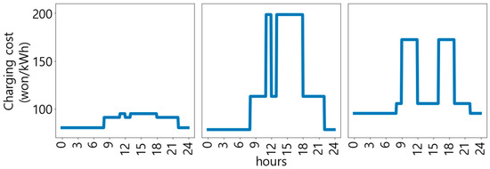
Figure 2.
Changes in charging cost by season and load hours.
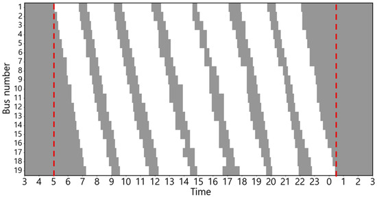
Figure 3.
Weekday operating pattern of Busan bus 41.
The parameters used to estimate the EB energy consumption are listed in Table 2. The parameters and in Equation (14) are used to calculate the energy consumption based on the driving speed, with values of and , respectively [29]. The parameters , and in Equation (15) were set to 0.7199, 11.977, 0.9163, 0.3665, and −6.1087, respectively [30]. Here, the heating start temperature was set to 15 °C and the cooling start temperature to 20 °C.
Table 2.
Parameters for estimating EB energy consumption.
The parameters used to calculate the battery aging cost are listed in Table 3. The parameters of cycle aging (, , ) and calendar aging (, , ) in Equations (4) and (5) were set to , , , , , , respectively [26]. The EOL in Equation (3) was set to 0.75, and , representing the decline in the value at resale, was set to 0.7.
Table 3.
Parameters for calculating EB energy consumption and battery capacity loss rate.
The parameter values for Scenario 2, 3 are listed in Table 4. The unit price per battery capacity () and battery capacity () were set to and , respectively. All EBs are serviced at the single depot located at the start/end points of the route. The number of chargers () in the depot was set to 4. The depot is equipped with fast chargers. In addition, EBs are also fast charging. The maximum charging power of the chargers and one EB () was set to . The parameters for constraining the upper and lower bounds of the battery SoC for all EBs (, ) were set to 0.2 and 0.8, respectively. The 235th time slot was selected as to when the last dispatched EB returned to the depot (). The total number of time slots to schedule charging () was 288, divided into 5 min intervals from 5 a.m., the time of the first dispatch, to 5:00 a.m. the next day. The minimum time slot of the interval between charges and the charging duration for each bus () was set to 3 [28,29]. The constants used for converting power to wattage () and wattage to battery SoC of the bus () were set to 0.0833 and , respectively.
Table 4.
Parameters for optimizing an EB charging schedule.
All scenario simulations were conducted with an Intel® Xeon® Gold 5320T CPU with 2.3 GHz and 128 Gb of RAM, and the optimization solver CPLEX Optimization Studio V12.8 was used to solve the MILP models.
4.2. Case Study Results
A comparison of the charging and battery degradation costs for the two scenarios is shown in Figure 4. Here, the hatched portions of the bar plots correspond to the battery aging cost in Scenario 1, which was calculated retrospectively. Compared with Scenario 1, Scenario 2 exhibited a reduction in the overall operating cost of 1.43, 12.3, and 5.69% in the spring/fall, summer, and winter seasons, respectively. Similarly, a comparison of Scenario 3 with Scenario 2 exhibited a reduction 0.198%, 0.303%, and 0.210%, respectively. These findings underscore the necessity of a charging strategy that considers battery aging and TOU. The cost of battery degradation decreased by 0.998%, 1.24%, and 0.779% in spring/fall, summer, and winter seasons, respectively, for Scenario 3 compared to Scenario 1, and by 0.795%, 1.24%, and 0.845% compared to Scenario 2. During winter, when energy consumption is at highest, the feasibility of implementing charging shifting is significantly constrained, thereby yielding minimal cost savings from battery degradation. During the spring/fall, energy consumption reaches its lowest, resulting in a relatively limited potential for cost savings, which in turn limits the overall impact of these savings. Consequently, it can be deduced that the savings rate is at its zenith during the summer. Charging costs decreased by 1.72%, 17.2%, and 7.82% in spring/fall, summer, and winter seasons, respectively, for Scenario 3 compared to Scenario 1. This demonstrates the most significant reduction during summer, when the disparity between off-peak and on-peak load charging costs is at its zenith. This is due to the fact that Scenario 1 did not take into account TOU. Additionally, the cost of charging in Scenario 3 exhibited an increase of 0.209%, 0.204%, and 0.0896% seasonally compared to Scenario 2. This finding suggests that Scenario 3, which was designed to achieve an overall reduction in operational costs, led to a reduction in battery degradation costs through the implementation of charging schedule adjustments. However, this was accompanied by a marginal increase in charging costs. Furthermore, the seasonal reduction rates are inversely proportional to energy consumption and charge/discharge volumes.
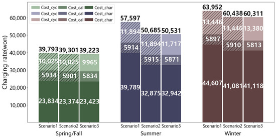
Figure 4.
Comparison of charging and battery degradation costs for one EB by scenario and season.
Figure 5 shows the daily energy consumption ratios for driving and cooling/heating according to the season. The percentage of the total energy consumption attributable to heating and cooling was higher in winter, summer, and spring, in that order: 29.58%, 20.39%, and 5.55%, respectively. Thus, the energy consumption for heating in winter was higher than the energy consumption for cooling in summer. These results indicate that heating and cooling systems should be considered when estimating the energy consumption of EBs.
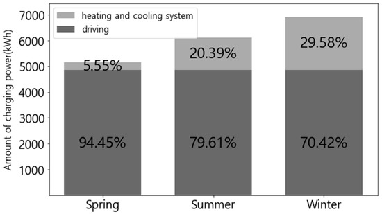
Figure 5.
Comparison of energy consumption by season. (The percentage written on each bar represents the ratio of the energy consumption due to the heating and cooling system and driving to the total energy consumption.).
The statuses of the EBs in the two scenarios are shown in Figure 6, Figure 7, Figure 8, Figure 9, Figure 10, Figure 11, Figure 12, Figure 13 and Figure 14. Here, white, grey, and black indicate the EB states for driving, waiting in the depot, and charging, respectively, and the dashed blue line indicates the end of the last EB operation. Smart charging was not applied in all scenarios; therefore, charging started immediately upon plug-in and ended when fully charged. Consequently, the EB was charged after the end of the last operation. In Scenario 1, the EBs charged during on-peak hours in all seasons. By contrast, Scenarios 2 and 3 incorporates a TOU charging cost, thereby ensuring that all EBs charged during on-peak hours exclusively in winter and some summer, when the energy consumption is at its peak. Details regarding the State of Charge (SoC) for each vehicle related to this is delineated in Figure A1, Figure A2, Figure A3, Figure A4, Figure A5, Figure A6, Figure A7, Figure A8 and Figure A9 in Appendix B. Notably, in Scenarios 2 and 3, an average of 37% of the EBs charged before the initial departure compared with 26% in Scenario 1. This result demonstrates the effectiveness of utilizing off-peak hours to minimize charging costs.
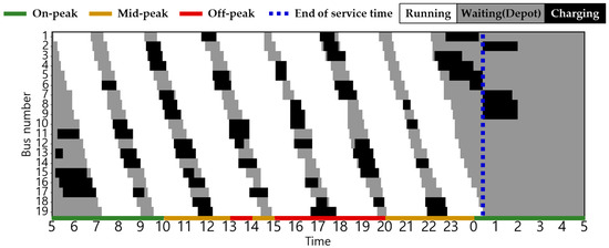
Figure 6.
EB operation pattern in Scenario 1 during spring/fall.
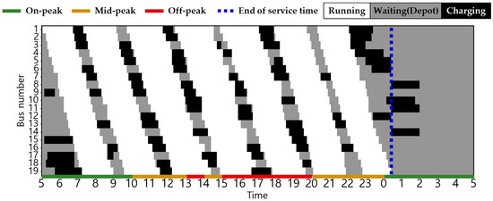
Figure 7.
EB operation pattern in Scenario 1 during summer.
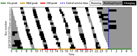
Figure 8.
EB operation pattern in Scenario 1 during winter.
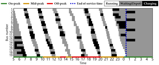
Figure 9.
EB operation pattern in Scenario 2 during spring/fall.
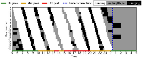
Figure 10.
EB operation pattern in Scenario 2 during summer.
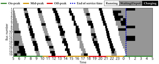
Figure 11.
EB operation pattern in Scenario 2 during winter.
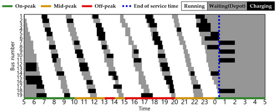
Figure 12.
EB operation pattern in Scenario 3 during spring/fall.
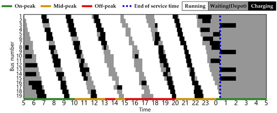
Figure 13.
EB operation pattern in Scenario 3 during summer.
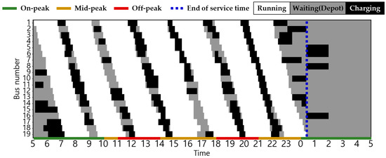
Figure 14.
EB operation pattern in Scenario 3 during winter.
Figure 15 shows the average battery SoC of EBs for each scenario and season. The average battery SoC for Scenario 3, which considered battery degradation, remained lower than that for Scenarios 1 and 2 for all seasons. This is because the battery SoC of EBs is affected by calendar aging. Although the dispatch schedule was the same for all seasons and scenarios, the energy consumptions per season differed. Consequently, the average battery SoC in Scenario 1, which did not consider the TOU charging cost, decreased in the order of spring/fall, summer, and winter. It was confirmed that the operating schedule of all seasons is the same, but it is inversely proportional accordingly because the energy consumption of each season is different. However, in Scenarios 2 and 3, where the TOU charging costs were considered, the average battery SoC decreased in the order of summer, winter, and spring/fall. The reason for the lowest value in winter is because energy consumption is highest. In addition, the average battery SoC is highest during summer, likely due to charging schedule adjustments to avoid peak load hours. This is due to the fact that the peak load rate during the summer season is the highest, although the total peak load hours for all seasons remain constant at six h.
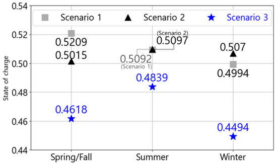
Figure 15.
Comparison of average SoC by scenario.
The hourly variations in the average battery SoC of EBs for each scenario and season is shown in Figure 16, Figure 17 and Figure 18. In spring/fall, each scenario has similar overall charging patterns, but Scenario 3 has lower values in all time zones, except at 8 a.m. This is because the calendar aging considered in Scenario 3 maintained the battery SoC at low. In addition, in spring/fall, the average battery SoC at the start of the charging schedule was approximately 59% in Scenario 1 and 53% in Scenario 3, which was the largest difference compared with that in the other seasons. This is attributed to the lowest energy consumption in spring/fall, allowing for more flexibility in the same charging time. In summer, the average battery SoC of the EBs was higher from 8 a.m. to 2 p.m. in Scenario 3 than that in Scenario 1, and Scenario 2 was also high, including this time zone and after 12 a.m. This can be attributed to the reduction in charging during peak loads from 3 p.m. to 8 p.m. In addition, the average battery SoC in Scenario 2 reached approximately 67% from 10 a.m.to 11 a.m., which was the highest value for all seasons and scenarios. In winter, the overall charging patterns for each scenario were similar, with the average battery SoC of EBs in Scenario 3 being lowest in all time zones, except at 8 a.m. This suggests that the calendar aging considered in Scenario 3 maintained the battery SoC at low. In addition, in winter, the difference in values between each scenario was the smallest compared with that in the other seasons, which can be attributed to the highest energy consumption in winter.
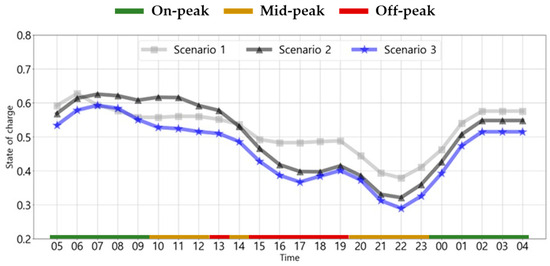
Figure 16.
Hourly variations in the average battery SoC of EBs for each scenario in spring/fall.
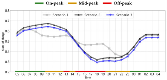
Figure 17.
Hourly variations in the average battery SoC of EBs for each scenario in summer.
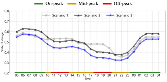
Figure 18.
Hourly variations in the average battery SoC of EBs for each scenario in winter.
5. Conclusions
The case study presented in this study revealed that heating and cooling energy consumption accounted for up to 29.58% of the total EB energy consumption. As indicated by the findings of the reviewed studies, neglecting this factor can lead to deviations in the EB battery SoC state beyond stable operational thresholds or result in increased charging costs. Moreover, the exclusion of calendar aging may cause an underestimation of end-of-life battery disposal or replacement costs. As demonstrated in this study, the adoption of the EB charging strategy, which integrates heating and cooling energy consumption into the total energy consumption while simultaneously accounting for both cycle and calendar aging, reduced operating costs by up to 12.3%. These findings underscore the imperative for an operational framework that comprehensively considers heating and cooling systems alongside periodic aging and calendar aging phenomena to ensure cost-effective operation and optimal battery life for EB. Consequently, EB operators can achieve reduced charging costs and overall operational efficiency improvements by incorporating these additional factors into their operations.
In this study, the focus was on short-term operational efficiency by minimizing daily operation costs, excluding Capital Expenditures (CAPEX), and applying the case study deterministically due to actual fixed route allocation. Future work will address these limitations by incorporating operational uncertainty and validating the model’s prediction accuracy using real-world bus operation data. It will also include a long-term cost analysis that considers CAPEX, battery warranty and replacement costs, second-life applications of aged batteries as energy storage systems (ESS), and vehicle-to-grid (V2G) integrated operation scenarios.
Author Contributions
Conceptualization, Y.-B.S. and S.-Y.S.; methodology, Y.-B.S. and S.-W.P.; software, Y.-B.S.; validation, S.-W.P. and S.-Y.S.; formal analysis, Y.-B.S. and S.-W.P.; investigation, Y.-B.S.; resources, Y.-B.S.; data curation, Y.-B.S. and S.-W.P.; writing—original draft preparation, Y.-B.S.; writing—review and editing, S.-W.P. and S.-Y.S.; visualization, Y.-B.S.; supervision, S.-Y.S.; project administration, S.-Y.S.; funding acquisition, S.-Y.S. All authors have read and agreed to the published version of the manuscript.
Funding
This work is supported by the Ministry of Trade, Industry and Energy (Grant No. 20214000000060, 50% and No. RS-2024-00419642, 50%) supervised by the KETEP (Korea Institute of Energy Technology Evaluation and Planning).
Data Availability Statement
The data presented in this study are available in reference number [30,31,32,33,34]. These data were derived from the following resources available in the public domain: https://online.kepco.co.kr/PRM004D00 (accessed on 1 August 2025), https://data.kma.go.kr/data/grnd/selectAsosRltmList.do?pgmNo=36 (accessed on 1 August 2025), http://bus.busan.go.kr/ (accessed on 1 August 2025), https://map.kakao.com/ (accessed on 1 August 2025), and https://www.data.go.kr/tcs/dss/selectApiDataDetailView.do?publicDataPk=15098533 (accessed on 1 August 2025).
Conflicts of Interest
The authors declare no conflict of interest.
Abbreviations
| Time interval suffix number. | |
| Total number of time slots. | |
| EB suffix number. | |
| Total number of EBs. | |
| Trip suffix number. | |
| Total number of trips. |
Appendix A
- Input variables
- : Total energy consumed by whether EB is garaged or waiting at time (0–1 binary, waiting = 1).: Amount of energy consumed by EB driving at time .: Amount of energy consumed by EB for heating and cooling at time .: Distance of route covered by EB .: Trip time for EB ’s trip.: EB ambient temperature at time .: Heating start temperature.: Cooling start temperature.: Charging cost for each load hour at time .: Battery unit cost per kWh.: Battery capacity of EB, .: End of battery life criteria.: Weighting to account for depreciation when selling used batteries.: Parameters based on cell temperature for estimating battery capacity loss due to cycle aging.: Cell temperature-dependent parameters for estimating battery capacity loss due to calendar aging.: DoD-specific parameters for estimating battery capacity loss due to cycle aging.: SoC-specific parameters for estimating battery capacity loss due to calendar aging.: Lower bound SoC.: Upper limit SoC.: Minimum number of charge duration intervals.: Total number of chargers.: Maximum charging power.: Time suffix number at which all operations end.: Time interval number at which the charging schedule ends.: Constant to convert power to the amount of power used during .: Constant for converting power to SoC value on the EB.: Whether EB is garaged or waiting at time (0–1 binary, waiting = 1).
- Decision variable
- : Charging power of EB at time : SoC on EB at time .: Percentage loss of battery capacity on EB at time .: Percentage of battery capacity loss due to cycle aging on EB at time .: Percentage of battery capacity loss due to calendar aging on EB at time .: Whether EB is charging at time (0–1 binary, charging = 1).: Whether EB starts charging at time (0–1 binary, start = 1).: Whether EB is terminating charging at time (0–1 binary, end = 1).
Appendix B
The following figures are as follows: Battery SoC by bus for different scenarios and seasons (with higher values indicating higher charge).

Figure A1.
Seasonal (Spring/Fall) Changes in Battery SoC Status for Scenario 1 (with higher values indicating higher charge).

Figure A2.
Seasonal (Summer) Changes in Battery SoC Status for Scenario 1 (with higher values indicating higher charge).

Figure A3.
Seasonal (Winter) Changes in Battery SoC Status for Scenario 1 (with higher values indicating higher charge).

Figure A4.
Seasonal (Spring/Fall) Changes in Battery SoC Status for Scenario 2 (with higher values indicating higher charge).

Figure A5.
Seasonal (Summer) Changes in Battery SoC Status for Scenario 2 (with higher values indicating higher charge).

Figure A6.
Seasonal (Winter) Changes in Battery SoC Status for Scenario 2 (with higher values indicating higher charge).

Figure A7.
Seasonal (Spring/Fall) Changes in Battery SoC Status for Scenario 3 (with higher values indicating higher charge).

Figure A8.
Seasonal (Summer) Changes in Battery SoC Status for Scenario 3 (with higher values indicating higher charge).

Figure A9.
Seasonal (Winter) Changes in Battery SoC Status for Scenario 3 (with higher values indicating higher charge).
References
- IEA. Available online: https://www.iea.org/energy-system/transport (accessed on 1 August 2025).
- Statista. Available online: https://www.statista.com/statistics/1129656/global-share-of-co2-emissions-from-fossil-fuel-and-cement/ (accessed on 1 August 2025).
- Borne, I.; Souza, S.A.S.d.; Carniatto Silva, E.T.; Soares, G.B.; Gimenez Ledesma, J.J.; Ando Junior, O.H. Sustainable mobility: Analysis of the implementation of electric bus in university transportation. Energies 2025, 18, 2195. [Google Scholar] [CrossRef]
- Bao, Z.Y.; Li, J.P.; Bai, X.H.; Xie, C.; Chen, Z.B.; Xu, M.; Shang, W.L.; Li, H.L. An optimal charging scheduling model and algorithm for electric buses. Appl. Energy 2023, 332, 120512. [Google Scholar] [CrossRef]
- Zheng, F.F.; Wang, Z.J.; Liu, M. Overnight charging scheduling of battery electric buses with uncertain charging time. Oper. Res. 2022, 22, 4865–4903. [Google Scholar] [CrossRef]
- Diego, C.; Jakub, G.; Christian, M. Energy Logistics Cost Study for Wireless Charging Transportation Networks. Sustainability 2021, 13, 5986. [Google Scholar] [CrossRef]
- Li, T.T.; Zhang, W.C.; Huang, G.S.; He, H.C.; Xie, Y.; Zhu, T.X.; Liu, G.T. Real-world data-driven charging strategies for incorporating health awareness in electric buses. J. Energy Storage 2024, 92, 112064. [Google Scholar] [CrossRef]
- Jin, K.; Li, X.R.; Wang, W.; Hua, X.D. Cost-Optimal Charging Strategies for electric bus Fleets Considering Battery Degradation and Nonlinear Charging. IEEE Trans. Intell. Transp. Syst. 2024, 25, 6212–6222. [Google Scholar] [CrossRef]
- Houbbadi, A.; Redondo-Iglesias, E.; Pelissier, S.; Trigui, R.; Bouton, T. Smart charging of electric bus fleet minimizing battery degradation at extreme temperature conditions. In Proceedings of the 2021 IEEE Vehicle Power and Propulsion Conference (VPPC), Gijon, Spain, 25–28 October 2021. [Google Scholar]
- Ma, X.L.; Miao, R.; Wu, X.K.; Liu, X.L. Examining influential factors on the energy consumption of electric and diesel buses: A data-driven analysis of large-scale public transit network in Beijing. Energy 2021, 216, 119196. [Google Scholar] [CrossRef]
- Wang, G.; Fang, Z.H.; Xie, X.Y.; Wang, S.; Sun, H.J.; Zhang, F.; Liu, Y.H.; Zhang, D.S. Pricing-aware Real-time Charging Scheduling and Charging Station Expansion for Large-scale electric buses. ACM Trans. Intell. Syst. Technol. 2021, 12, 26. [Google Scholar] [CrossRef]
- Liu, X.H.; Qu, X.B.; Ma, X.L. Optimizing electric bus charging infrastructure considering power matching and seasonality. Transp. Res. Part D Transp. Environ. 2021, 100, 103057. [Google Scholar] [CrossRef]
- Cigarini, F.; Schminkel, P.; Sonnekalb, M.; Best, P.; Göhlich, D. Determination of improved climatic conditions for thermal comfort and energy efficiency in electric buses. Appl. Ergon. 2022, 105, 103856. [Google Scholar] [CrossRef]
- Xing, Y.; Fu, Q.B.; Li, Y.C.; Chu, H.S.; Niu, E.Y. Optimal Model of electric bus Scheduling Based on Energy Consumption and Battery Loss. Sustainability 2023, 15, 9640. [Google Scholar] [CrossRef]
- Würtz, S.; Bogenberger, K.; Göhner, U.; Rupp, A. Towards Efficient Battery electric bus Operations: A Novel Energy Forecasting Framework. World Electr. Veh. J. 2024, 15, 27. [Google Scholar] [CrossRef]
- Zaneti, L.A.L.; Arias, N.B.; de Almeida, M.C.; Rider, M.J. Sustainable charging schedule of electric buses in a University Campus: A rolling horizon approach. Renew. Sustain. Energy Rev. 2022, 161, 112276. [Google Scholar] [CrossRef]
- Chen, Q.Z.; Niu, C.M.; Tu, R.; Li, T.Z.; Wang, A.; He, D.B. Cost-effective electric bus resource assignment based on optimized charging and decision robustness. Transp. Res. Part D Transp. Environ. 2023, 118, 103724. [Google Scholar] [CrossRef]
- Li, P.S.; Jiang, M.Y.; Zhang, Y. Cooperative Optimization of Bus Service and Charging Schedules for a Fast-Charging Battery electric bus Network. IEEE Trans. Intell. Transp. Syst. 2023, 24, 5362–5375. [Google Scholar] [CrossRef]
- Fan, D.M.; Feng, Q.; Zhang, A.B.; Liu, M.M.; Ren, Y.; Wang, Y.P. Optimization of Scheduling and Timetabling for Multiple Electric Bus Lines Considering Nonlinear Energy Consumption Model. IEEE Trans. Intell. Transp. Syst. 2024, 25, 5342–5355. [Google Scholar] [CrossRef]
- Zhang, L.; Wang, S.A.; Qu, X.B. Optimal electric bus fleet scheduling considering battery degradation and non-linear charging profile. Transp. Res. Part E Logist. Transp. Rev. 2021, 154, 102445. [Google Scholar] [CrossRef]
- Zhou, Y.; Meng, Q.; Ong, G.P. Electric bus Charging Scheduling for a Single Public Transport Route Considering Nonlinear Charging Profile and Battery Degradation Effect. Transp. Res. Part B Methodol. 2022, 159, 49–75. [Google Scholar] [CrossRef]
- Saner, C.B.; Trivedi, A.; Srinivasan, D. A Multi-Module Modeling and Optimization Framework for Integrated Planning and Operation of electric bus Shuttle Fleets. IEEE Trans. Intell. Transp. Syst. 2024, 25, 16910–16924. [Google Scholar] [CrossRef]
- Gkiotsalitis, K.; Rizopoulos, D.; Merakou, M.; Iliopoulou, C.; Liu, T.; Cats, O. Electric bus charging station location selection problem with slow and fast charging. Appl. Energy 2025, 382, 125242. [Google Scholar] [CrossRef]
- Jiang, M.Y.; Zhang, Y.; Zhang, Y. A Branch-and-Price Algorithm for Large-Scale Multidepot Electric Bus Scheduling. IEEE Trans. Intell. Transp. Syst. 2023, 24, 15355–15368. [Google Scholar] [CrossRef]
- Sayfutdinov, T.; Ali, M.; Khamisov, O. Alternating direction method of multipliers for the optimal siting, sizing, and technology selection of Li-ion battery storage. Electr. Power Syst. Res. 2020, 185, 106388. [Google Scholar] [CrossRef]
- Tomizawa, Y.; Ihara, Y.; Kodama, Y.; Iino, Y.; Hayashi, Y.; Ikeda, O.; Yoshinaga, J. Multipurpose Charging Schedule Optimization Method for electric buses: Evaluation Using Real City Data. IEEE Access 2022, 10, 56067–56080. [Google Scholar] [CrossRef]
- Hu, H.; Du, B.; Liu, W.; Perez, P. A joint optimisation model for charger locating and electric bus charging scheduling considering opportunity fast charging and uncertainties. Transp. Res. Part C Emerg. Technol. 2022, 141, 103732. [Google Scholar] [CrossRef]
- Basma, H.; Mansour, C.; Haddad, M.; Nemer, M.; Stabat, P. Comprehensive energy modeling methodology for battery electric buses. Energy 2020, 207, 118241. [Google Scholar] [CrossRef]
- Perugu, H.; Collier, S.; Tan, Y.; Yoon, S.; Herner, J. Characterization of battery electric transit bus energy consumption by temporal and speed variation. Energy 2023, 263, 125914. [Google Scholar] [CrossRef]
- Electricity Table KEPCO ON. Available online: https://online.kepco.co.kr/PRM004D00 (accessed on 1 August 2025).
- Weather Data Opening Portal KMA. Available online: https://data.kma.go.kr/data/grnd/selectAsosRltmList.do?pgmNo=36 (accessed on 1 August 2025).
- Busan Bus Information Management System. Available online: http://bus.busan.go.kr/ (accessed on 1 August 2025).
- Kakao Map. Available online: https://map.kakao.com/ (accessed on 1 August 2025).
- Ministry of Land, Infrastructure and Transport_(TAGO)_Bus Location Information, Public Data Portal. Available online: https://www.data.go.kr/tcs/dss/selectApiDataDetailView.do?publicDataPk=15098533 (accessed on 1 August 2025).
Disclaimer/Publisher’s Note: The statements, opinions and data contained in all publications are solely those of the individual author(s) and contributor(s) and not of MDPI and/or the editor(s). MDPI and/or the editor(s) disclaim responsibility for any injury to people or property resulting from any ideas, methods, instructions or products referred to in the content. |
© 2025 by the authors. Licensee MDPI, Basel, Switzerland. This article is an open access article distributed under the terms and conditions of the Creative Commons Attribution (CC BY) license (https://creativecommons.org/licenses/by/4.0/).