1. Introduction
Container trucks constitute the primary mode of cargo transport in port cities. However, their heavy dependence on diesel fuel results in considerable emissions of air pollutants and carbon dioxide, generating not only localized impacts within port areas but also contributing to city-wide air quality degradation and heightened urban carbon burdens [
1].
To address these challenges, liquefied natural gas (LNG) container trucks, which offer distinct low-carbon and economic advantages, have been identified as a promising option [
2,
3,
4] for reducing emissions and improving air quality. Compared with conventional diesel trucks, they significantly reduce nitrogen oxides and particulate matter and achieve about a 10% reduction in CO
2 emissions [
5]. Given these environmental benefits, it is crucial to identify the factors that influence their carbon emissions and to quantify the contributions of these factors to overall emissions. This study aims to provide the scientific basis for promoting the wider adoption of LNG container trucks and for developing targeted emission control strategies to mitigate pollution in port-adjacent cities. Existing studies on vehicle emissions can be broadly categorized into macroscopic and microscopic approaches. At the macroscopic level, the top-down method estimates emissions at national or regional scales using fuel sales data from specific areas. Research has evaluated the CO
2 emissions of conventional diesel and liquefied natural gas heavy-duty vehicles (LNG HDVs), highlighting key factors that influence overall greenhouse gas outputs [
6]. At the microscopic level, the bottom-up method requires more detailed datasets, including vehicle-specific characteristics and mileage traveled by individual vehicles. Studies have analyzed the fuel consumption and exhaust emissions of diesel vehicles under different road conditions, applying vehicle-specific power (VSP) models to estimate road load and regression coefficients [
7].
Laboratory simulations are an important method for assessing vehicle carbon emissions, with controlled tests and engine bench experiments widely used to evaluate emissions under standardized operating conditions. At the same time, modeling has advanced through the development of bottom-up life-cycle models, which estimate the total energy use and greenhouse gas (GHG) emissions of diesel and LNG heavy-duty vehicles across both fuel and vehicle life-cycle stages [
8]. In addition to controlled experiments and statistical analyses, researchers have increasingly relied on real-world emission measurements and modeling approaches. Portable Emission Measurement Systems (PEMS), which allow for direct sampling and on-road monitoring of exhaust emissions, have been widely applied in diesel and hybrid vehicle studies, providing valuable data under actual driving conditions [
9,
10,
11,
12,
13]. These empirical findings have further informed the calibration and validation of emission models, thereby enhancing the accuracy of emission inventories and policy evaluations.
In summary, previous studies have made valuable contributions by highlighting the energy-saving and emission-reduction potential of natural gas heavy-duty vehicles. However, the emission characteristics and influencing factors of LNG container trucks in the complex port hinterland environment remain underexplored. Particularly, the effects of traffic congestion, road types, and ramp slopes on CO2 emissions are insufficiently studied. This paper investigated the emission characteristics of LNG container trucks through real-world road tests, focusing on the relationship between traffic congestion and CO2 emissions on elevated roads, and the impact of ramp slopes, providing a scientific basis for the energy saving and emission reduction of clean energy vehicles in port transportation.
2. Experimental Setup and Calculation Methods
2.1. Test Vehicle and Routes
The experimental vehicle in this study was an LNG container truck produced in 2023, complying with China VI emission standards [
14]. Relevant information and specifications are listed in
Table 1. To minimize the influence of variations in driving style on the experimental results, all test conditions were conducted by a single driver to ensure consistency in driving operations. The weight of the LNG container truck during the experiment was 7.3 ton. Generally, vehicles with a longer service life and a greater mileage tend to have higher emissions than those with shorter service life and mileage [
15]. The vehicles used in this study started operation in 2023 and had a mileage of less than 10,000 km. Therefore, the findings presented in this paper reflect the emission characteristics of the vehicles during their initial stage of use.
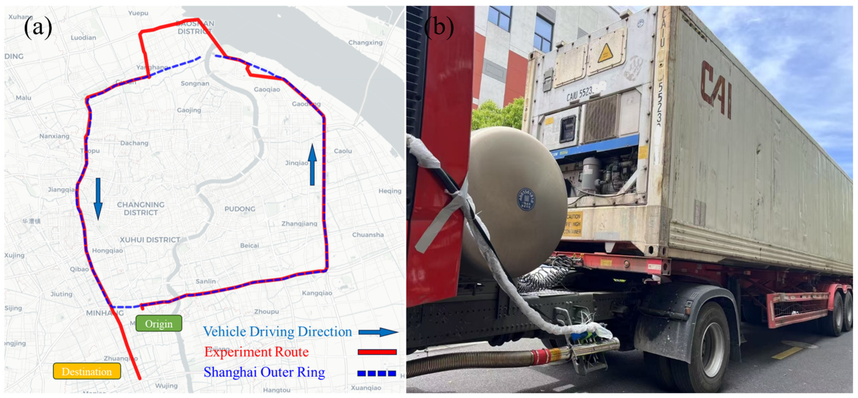
The experiment was conducted in Shanghai on 8 May 2024 (15:00–22:00) and 9 May 2024 (11:00–18:00), covering an approximately 80 km closed-loop route. The route traveled via the Outer Ring Expressway to the Outer Fifth/Outer Fourth Terminals and then returned via the Outer Ring Expressway, which was shown in
Figure 1. Due to Shanghai’s local restrictions on heavy trucks, container trucks were unable to enter urban roads within the Outer Ring Road. Therefore, the experimental route planning excluded urban roads.
The route primarily consisted of the main expressway (free-flowing speed = 80 km/h) and ramp connections, covering a variety of typical operating conditions, including peak and off-peak traffic. Based on real-time vehicle speed and congestion index, the data was divided into three operating conditions: unobstructed traffic (vehicle speed > 40 km/h, congestion index < 20%), congestion (24 km/h < vehicle speed≤ 40 km/h, congestion index 20–50%), and severe congestion (vehicle speed ≤ 24 km/h, congestion index > 50%). Combined with elevation data, comparative analysis was conducted for level roads, uphill sections (entering elevated ramps), and downhill sections (descending elevated ramps).
2.2. Carbon Emission Measurement System
In this study, a vehicle-mounted Portable Emission Measurement System (PEMS) was installed in the driver’s cabin to record real-time emissions at 1 Hz, and was applied to quantify the CO2 emissions of an LNG container truck under actual road conditions.
During data collection, the system synchronized three key types of data: emissions data, vehicle operating parameters and environmental data. During data collection, the system synchronized three key types of data: emissions data, vehicle operating parameters and environmental data. Vehicle operating parameters (engine speed, throttle position) were synchronously recorded through the OBD interface, GPS positioning system tracked vehicle speed and driving trajectory, PEMS built-in meteorological module and vehicle dashcam collected temperature, humidity, atmospheric pressure, and road condition videos. Supplementary meteorological data came from fixed monitoring stations around Shanghai and portable weather instruments. All equipment was calibrated and statically verified on 8 May 2024 and 9 May 2024, ensuring CO2 measurement accuracy of ±2% and particle number concentration measurement error <5%.
2.3. Methods
2.3.1. Calculation of Vehicle Specific Power (VSP)
Vehicle Specific Power (VSP) is an important indicator that describes the instantaneous power demand per unit mass of a vehicle during driving [
16,
17,
18]. It can comprehensively reflect the impact of acceleration, aerodynamic drag, tire rolling resistance, and road gradient on emissions. In the MOVES [
19] model developed by USEPA, the VSP calculation formula for diesel medium and heavy-duty passenger vehicles is as follows, and this formula is also used in the calculation of VSP for LNG trucks:
where v is the instantaneous vehicle speed (m/s); a is the acceleration (m/s
2); g is the acceleration due to gravity (9.81 m/s
2); θ is the vertical ascent of the vehicle divided by the slope length. The gradient on the elevated road is very small, which is assumed to be 0. Because this study analyzes the emission data collected on ramps or bridges separately, the height of the elevated road is designed according to the specifications, and the slope changes are ignored.
In order to enhance the accuracy of data analysis and the robustness of the results, this study uses the interval method to classify VSP. By dividing the continuous VSP values into intervals, the average emission level in each interval can be determined more accurately, and in-depth analysis can be carried out in combination with the VSP distribution characteristics. Considering the need to reduce data aggregation errors and reduce computational complexity, this study chooses to bin the VSP at intervals of 2 kW/t. The binning method [
20,
21] is shown in Formula (2):
where n was any integer value.
2.3.2. Determination on the Feature Importance of CO2 Emission
To accurately identify the key factors influencing vehicle CO2 emissions, this study categorized all input features into three main categories based on their physical significance and operational mechanisms for systematic analysis. Engine behavior features include throttle position, engine speed, fuel rate, exhaust temperature, and exhaust volume flow rate. These parameters directly reflect the internal combustion process and thermodynamic state of the engine. Driving behavior features include vehicle speed and VSP, representing vehicle operating conditions and driver operating characteristics. External environmental features include weather probe humidity and ambient temperature, reflecting the impact of external conditions on emissions. This classification approach allows for a systematic assessment of the relative contributions of different types of factors to CO2 emission prediction.
To assess the potential impact of multicollinearity between features on model performance, this study calculated the variance inflation factor (VIF) [
22] for each feature under different traffic conditions. The VIF value is defined as:
where
Ri2 represents the coefficient of determination of the regression of the
i-th feature on all other features. This metric quantifies the degree to which a feature is linearly explained by other features. Higher VIF values indicate more severe multicollinearity. In this study, VIF analysis was employed as a preprocessing procedure rather than a direct modeling outcome. As shown in
Table 2, the VIF values for all features under various traffic conditions are below the critical threshold of 5, indicating that inter-feature collinearity has been effectively controlled and does not significantly impact the stability and interpretability of the model.
This study employed the SHAP [
23] method to conduct feature importance analysis on the machine learning model. This approach was based on the Shapley value concept from game theory and provides marginal contributions of each feature for every prediction outcome. By calculating the marginal contribution of each feature across all possible feature combinations, the SHAP method fairly allocated the responsibility of each feature to the final prediction results, overcoming the limitations of traditional feature importance methods in handling feature interactions. The SHAP analysis results not only provided a global ranking of feature importance but also visualized the specific impact direction and magnitude of each feature value range on model predictions through visualization, establishing a solid theoretical foundation for model interpretability.
2.3.3. CO2 Emission Prediction Model Based on XGBoost Method
XGBoost (eXtreme Gradient Boosting) [
24] is an advanced ensemble learning algorithm that implements gradient boosting of decision trees through significant computational optimization and regularization techniques. The algorithm builds a strong predictor by sequentially adding weak learners (typically decision trees) to minimize a differentiable loss function [
25,
26].
3. Results and Discussion
3.1. Impact of Traffic Behavior on CO2 Emission
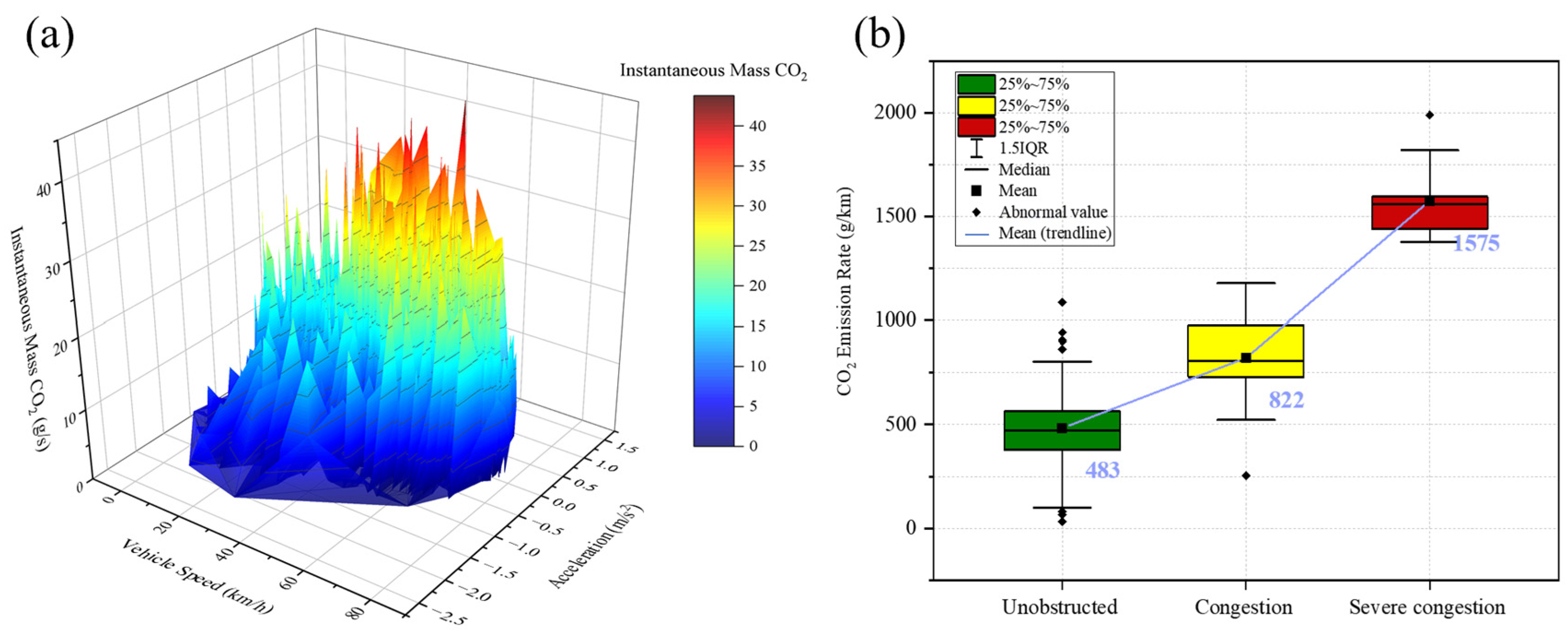
Figure 2a illustrated the nonlinear relationship between carbon emissions and speed-acceleration for natural gas container trucks. LNG trucks on elevated highways predominantly operated within the medium-to-high speed range (40–80 km/h). Carbon emissions exhibited a characteristic U-shaped distribution with respect to vehicle speed [
27,
28]: during low-speed operation (0–10 km/h), reduced engine efficiency and incomplete combustion resulted in elevated emissions; at medium speeds (30–50 km/h), engine thermal efficiency reached optimal conditions with the lowest carbon emissions per unit distance; while at high speeds (>60 km/h), dramatically increased aerodynamic drag and elevated engine power demands caused emissions to rise again. The acceleration process demonstrated a significant amplification effect on emissions, as increased engine load led to substantial increases in fuel injection rates [
29], with instantaneous emissions potentially increasing by 10–20% under rapid acceleration conditions. The surface plot revealed a “peak-valley” distribution with multiple local extrema, indicating that emission behavior was subject to complex regulation through speed-acceleration coupling effects. Maintaining steady acceleration during high-speed operation could effectively reduce emission peaks, while frequent acceleration-deceleration maneuvers significantly deteriorated emission levels [
30,
31]. These nonlinear characteristics provided supporting evidence for the subsequent application of XGBoost methods to capture complex emission mechanisms and offered theoretical foundations for optimizing energy-saving and emission-reduction strategies for LNG container trucks on elevated highways.
Figure 2b revealed significant differences in CO
2 emissions from LNG container trucks under three traffic congestion conditions. The average emission factor under unobstructed conditions was 482.65 g/km, rising to 821.55 g/km under congestion, a 70.2% increase compared to unobstructed conditions. Under severe congestion, the emission factor rose further to 1575.43 g/km, a 226.4% increase compared to unobstructed conditions and a 91.7% increase compared to congestion. The change in the mean CO
2 emission factor clearly demonstrated an exponential growth trend with increasing traffic congestion severity [
32,
33]. Under severe congestion, frequent stop-and-go patterns, idling, and low-speed driving significantly reduced engine efficiency, exacerbated incomplete combustion and caused CO
2 emissions per mile to more than double compared to unobstructed conditions [
31].
Figure 3 illustrated the quadratic functional relationship between CO
2 emissions and VSP under different traffic conditions, along with their statistical characteristics. The four subplots represented unobstructed, congestion, severe congestion, and overall condition, respectively. Unobstructed condition exhibited the highest R
2 value (0.966), while congestion showed a decrease to R
2 = 0.783. Severe congestion condition demonstrated an R
2 recovery to 0.889, and overall condition yielded R
2 = 0.921. The lowest R
2 under congestion condition indicated that vehicles frequently alternate between free-flow and constrained states during this phase, with random driving behaviors such as micro-accelerations and brief braking making the emission patterns most complex. Conversely, although severe congestion presented the worst traffic conditions [
34], vehicles remained in relatively stable low-speed-idling cycles for extended periods, resulting in emission behaviors that exhibited certain regularities.
The intercept coefficients displayed a decreasing pattern: congestion showed the highest value (7.249), followed by free-flow conditions (6.258), overall conditions (5.873), and severe congestion with the lowest value (4.729). This phenomenon indicated that irregular driving behaviors such as frequent start-stop patterns and idling during congestion, generated the highest baseline emissions even in low VSP ranges. Although severe congestion presented the worst traffic conditions, vehicles maintained relatively stable low-speed or stationary states for extended periods, avoiding the frequent dynamic transitions characteristic of congestion, thus resulting in relatively lower baseline emissions. Analysis of the quadratic coefficients revealed that severe congestion exhibited the largest coefficient (0.067), indicating the most dramatic emission growth once entering high VSP ranges. Overall condition showed intermediate values (0.031), while congestion demonstrated the smallest coefficient (0.026), reflecting relatively gradual emission growth under high-load conditions. The overall condition eliminated the extreme characteristics of individual traffic states and presented smoother and more regular emission patterns, which exemplified the “regression to the mean” phenomenon under large-sample statistics [
35,
36]. Even when incorporating the complex and variable congestion conditions, the overall fitting quality remained at a high level (0.921), demonstrating that VSP served as a robust emission prediction indicator at the macroscopic scale.
3.2. Impact of Slope Behavior on CO2 Emission
In previous research [
31] on container truck carbon emissions, given Shanghai’s location on a plain and the relatively small slope of the elevated highway, the impact of slope was largely ignored when considering different road conditions, setting it to zero to simplify the complexities and focus on key issues. However, ignoring road grade can cause errors exceeding 25% in mesoscopic modeling of heavy-duty truck energy consumption and emissions [
37], making it necessary to reconsider this factor. On- and off-ramps, as essential components of the elevated highway, must be designed to strictly adhere to regulations and differ significantly from other sections of the elevated highway. Furthermore, these on- and off-ramps were often congested areas on the Shanghai Outer Ring Elevated Highway, making them highly valuable for research.
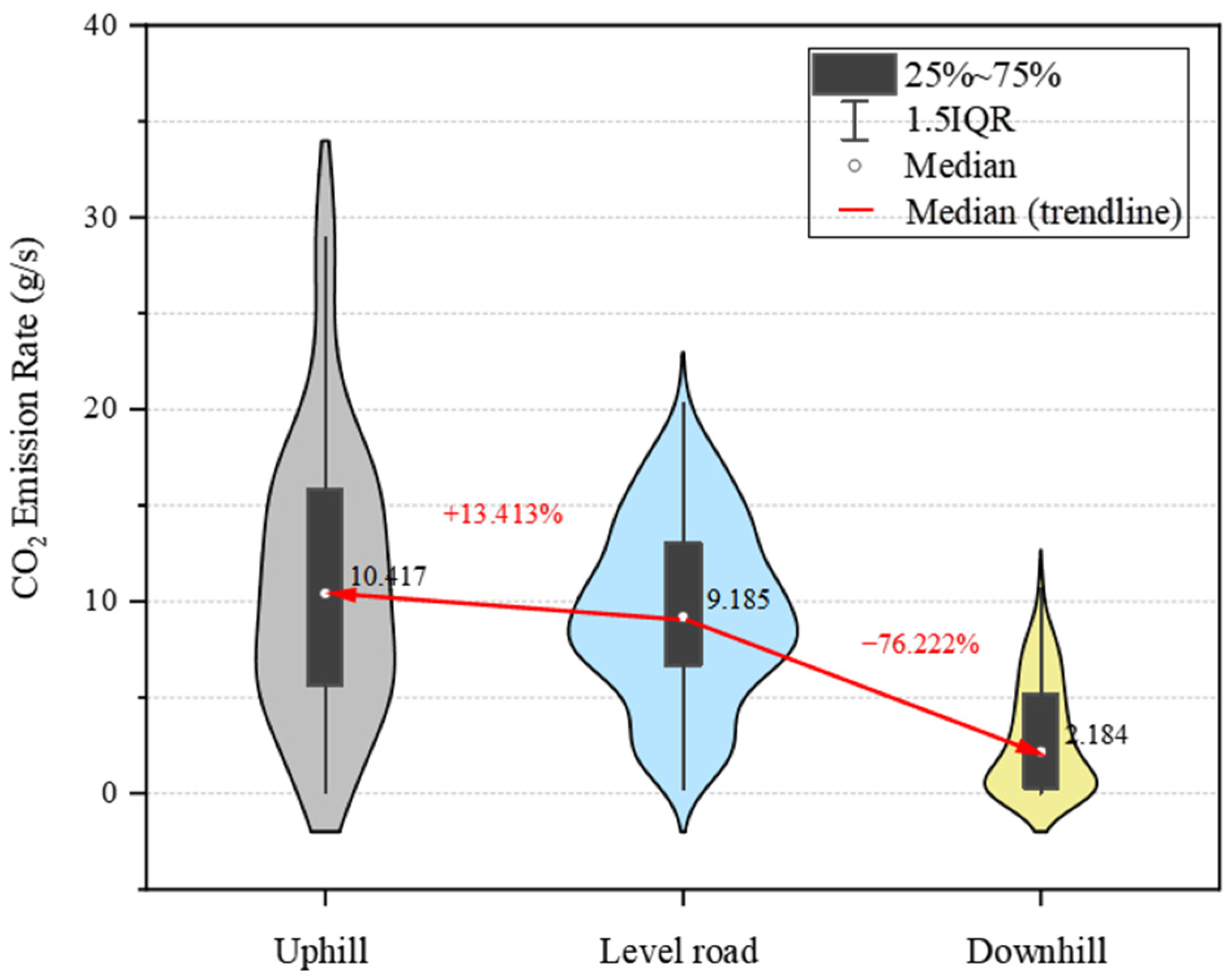
Figure 4 showed the statistical distribution and numerical trends of CO
2 emission factors for motor vehicles under three typical road conditions. The carbon emission factors for uphill, flat, and downhill conditions exhibited a clear step-by-step decreasing pattern. The median emission factor for flat roads was 9.185. The median emission factor for uphill driving reached 10.417, a 13.41% increase compared to the control group. The median emission factor for downhill driving was 2.184, a significant decrease of 76.22% compared to flat roads. The distribution of carbon emission factors on uphill slopes was characterized by a wide spindle shape and a large upward and downward extension range, with the highest data variability and uncertainty. This was because the vehicle needed additional power to overcome gravity when going uphill [
38]; the distribution of CO
2 emission factors on flat slopes was significantly narrowed, reflecting that when the slope was almost 0, there was no influence of gravity, the consistency of emission factors improved, and the impact of driving behavior was relatively controllable; the CO
2 emission factors in downhill condition changed most significantly, and the distribution showed obvious contraction and downward shift and was concentrated in the low value range, reflecting that the conversion of gravitational potential energy into kinetic energy greatly reduced the engine load [
39], and its high concentration indicated the strongest predictability.
3.3. Impact of Engine Behavior on CO2 Emission
Engine behavior is also an important characteristic factor affecting CO
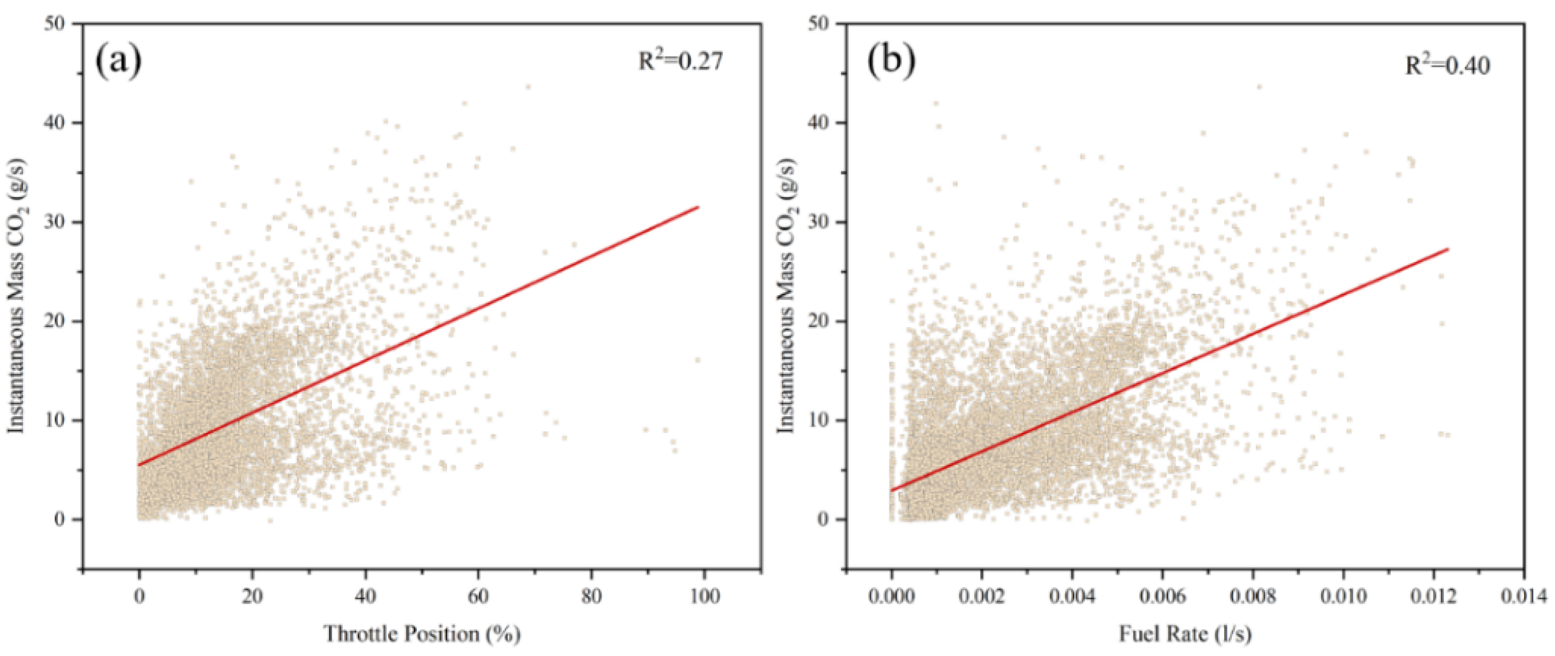
2 emissions. Throttle Position and Fuel Rate are selected as representatives to draw a relationship diagram.
Figure 5 showed that there is a clear nonlinear positive correlation between the CO
2 emission factor and both Throttle Position [
40] and Fuel Rate [
41].
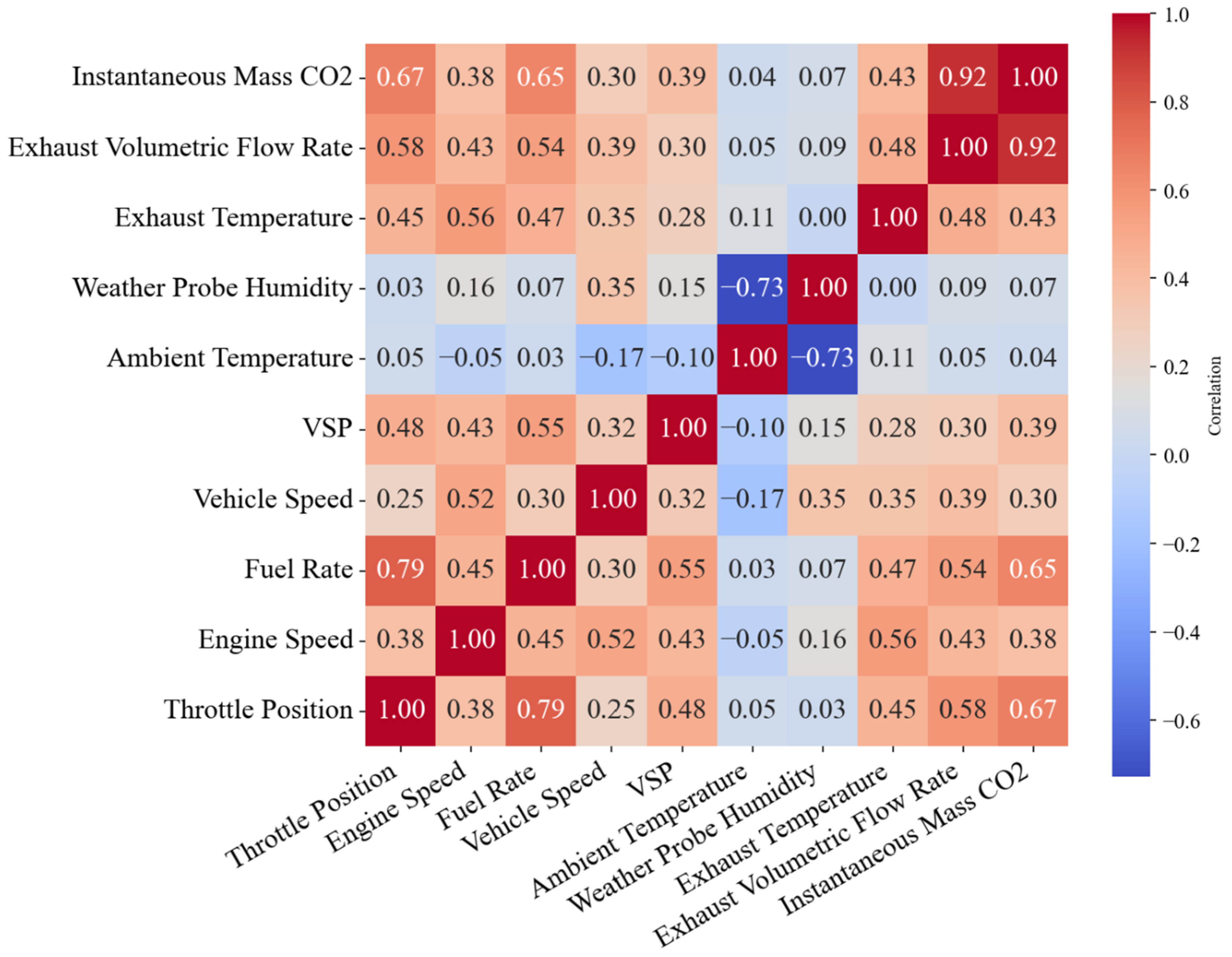
Quantitative analysis of the correlation matrix in
Figure 6 illustrated the strong correlation between engine parameters and CO
2 emissions. Exhaust volume flow rate exhibited a correlation coefficient of 0.92, surpassing the conventional threshold for super-strong correlation (r > 0.90). This result indicates that exhaust flow can serve as a near-deterministic indicator of CO
2 formation, directly reflecting the magnitude of combustion products. By comparison, throttle position (r = 0.67) and fuel consumption rate (r = 0.65) showed strong but less pronounced correlations, which is likely attributable to the influence of engine control strategies and transient driving conditions [
42]. Engine speed exhibited only a moderate correlation (r = 0.38), suggesting that its effect on CO
2 emissions is indirect, primarily mediated through variations in engine load and fuel injection rate.
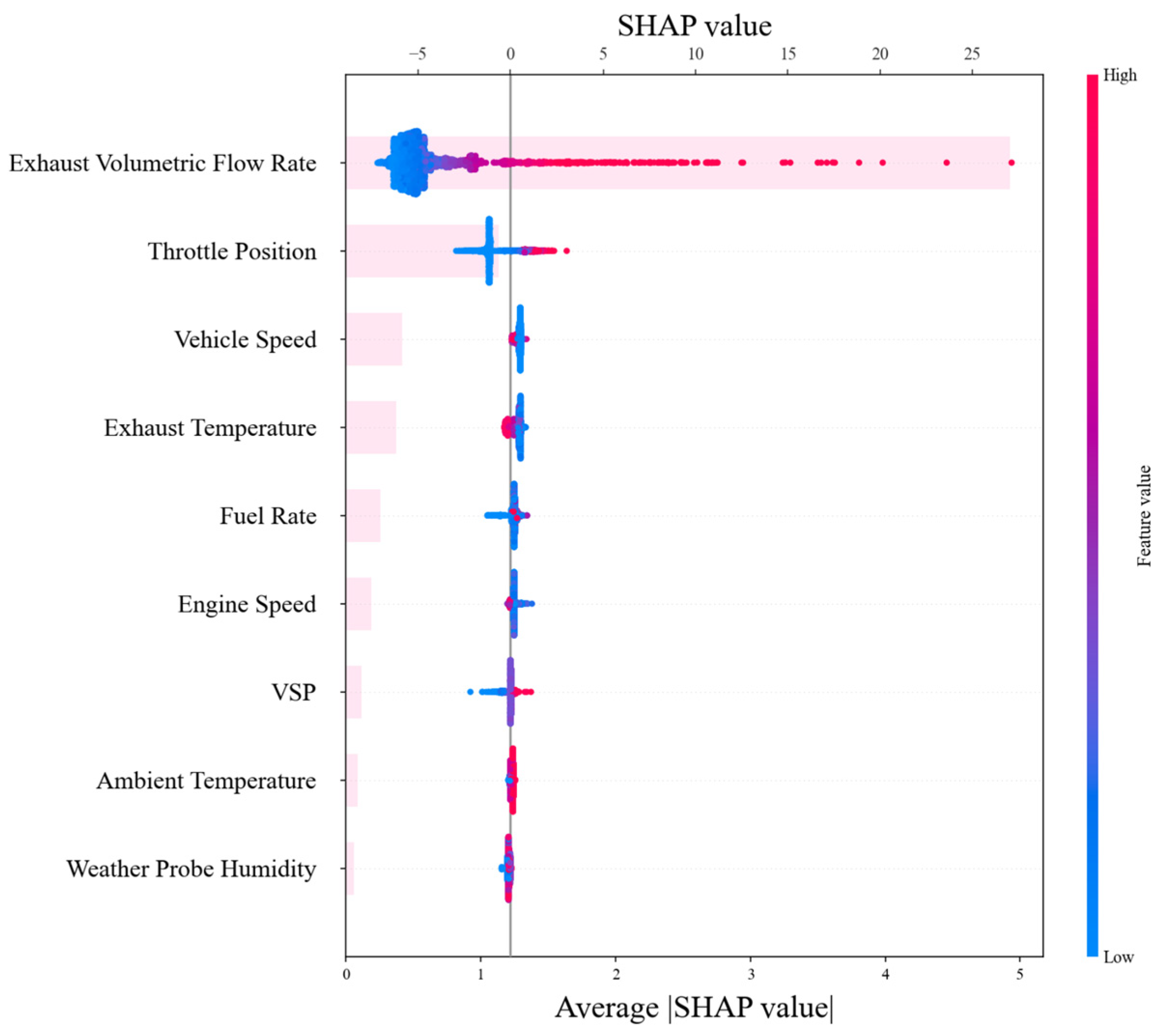
Figure 7 showed the numerical results of the SHAP importance analysis, further quantifying the predictive contribution of each engine parameter. The SHAP plot showed that exhaust volume flow rate had the highest average SHAP value, approximately 1.0, significantly exceeding all other features. Throttle position had an average SHAP value of approximately 0.4, ranking second, while exhaust temperature and fuel consumption rate had SHAP values of approximately 0.3 and 0.25, respectively. Engine speed and VSP had relatively low SHAP values, approximately 0.15–0.20. These numerical differences clearly reflected the weighting of different engine parameters in the model’s decision-making, with exhaust volume flow rate contributing 4–5 times more than less important features.
3.4. Estimation of CO2 Emission Using Machine Learning Method
To quantify the contribution of different feature dimensions to emission prediction accuracy, this study constructed two comparative models: an engine behavior feature model (including throttle position, engine speed, fuel consumption rate, exhaust temperature, and exhaust volume flow) and a full-feature integration model (which additionally incorporated driving behavior features: vehicle speed and specific power (VSP), and environmental feature: humidity and ambient temperature).
The prediction results of the model based solely on engine intrinsic parameters are shown in
Figure 8a. This model achieved an accuracy of R
2 = 0.966 with an RMSE of 1.173 g/s. The scatter plot demonstrated a strong linear correlation between predicted and measured values, with most data points distributed near the ideal fit line. These results indicated that directly measured parameters of the engine combustion process explained 96.6% of the variability in CO
2 emissions, thereby confirming the strong coupling between the engine’s intrinsic mechanisms and emissions output.
The prediction performance of the model can be further enhanced by comprehensively incorporating driving behavior and environmental features, as illustrated in
Figure 8b The R
2 increased to 0.982, and the RMSE decreased to 0.849 g/s, representing improvements of 1.66% and reductions of 27.6%, respectively, compared to the engine-only model. The scatter plot indicated that the data points were more tightly clustered around the ideal fit line, with significant improvements in fit accuracy, particularly in the mid-to-high emission range (20–40 g/s). This enhancement reflected the synergistic effect of multidimensional feature integration on emission prediction accuracy.
Model validation results demonstrated that while emission prediction based solely on engine parameters achieved good baseline performance, the limitations of feature dimensionality restricted the model’s accuracy under complex operating conditions. Multidimensional feature integration, through information complementarity and redundancy correction mechanisms, significantly enhanced the model’s generalization and stability, providing a reliable foundation for developing high-precision vehicle emissions prediction systems.
4. Conclusions
This study employed PEMS to conduct real-world emission measurements of LNG container trucks in Shanghai. The measurement study quantified the key factors influencing the instantaneous emission rates of China VI LNG container trucks, predicted their instantaneous CO2 emission rates, and derived distance-dependent CO2 emission factors. The main findings were summarized as follows:
Firstly, CO2 emissions exhibited a typical U-shaped distribution with vehicle speed of LNG container trucks operating on highways. Specifically, engine thermal efficiency was optimal and per-kilometer emissions were lowest at medium speeds (30–50 km/h), while emissions increased at both low and high speeds. Rapid acceleration increased instantaneous emissions by 10–20%. Emission factors varied significantly under different traffic conditions: the average emission factor under unobstructed conditions was 482.65 g/km, rising to 821.55 g/km (a 70.2% increase) under congestion and 1575.43 g/km (a 226.4% increase compared with unobstructed traffic) under severe congestion.
Secondly, engine-related factors were found to be the primary determinants of CO2 emissions, accounting for approximately 74% of total feature importance. Through correlation analysis, VIF tests, and SHAP importance analysis, the contribution of each factor on CO2 emissions was evaluated. Exhaust volumetric flow rate and exhaust temperature showed the strongest correlations with instantaneous CO2 mass emissions. Driving behavior factors accounted for about 20% of overall importance, while external environmental factors contributed only 6%. The XGBoost model demonstrated strong predictive capability, achieving R2 = 0.968 and RMSE = 1.139 on the full test set.
Thirdly, CO2 emissions from LNG container trucks on level roads, uphill segments, and downhill segments of elevated roads were qualified and compared. The median emission factor on level roads was 9.185 g/km. During uphill driving, it rose to 10.417 g/km, 13.41% higher than under level conditions. In contrast, during downhill driving, the median factor declined sharply to 2.184 g/km, representing a 76.22% reduction compared with level roads. Moreover, the on-ramp emission factor distribution exhibited the broadest spindle shape, reflecting the greatest variability and uncertainty among the three conditions.
In summary, this study conducted an in-depth investigation into the CO2 emissions of LNG container trucks and developed an efficient prediction model based on machine learning methods. The findings provided theoretical support and methodological guidance for the large-scale application of LNG trucks and for the development of high-precision vehicle emission prediction systems in future clean freight transport. Furthermore, the study on the emission characteristics of LNG container trucks conducted in this paper can provide a research basis for the life cycle assessment of LNG, enabling a better understanding of this green energy. However, this study was based on short-term data, so it might not provide a thorough understanding of long-term trends or seasonal variations. Future research can delve deeper into this issue.
Author Contributions
Conceptualization, Y.S. and H.H.; methodology, Y.S.; software, Y.S.; validation, H.Z., B.L. and L.L.; formal analysis, Y.S.; investigation, Y.S.; resources, H.Z.; data curation, Y.S.; writing—original draft preparation, H.Z.; writing—review and editing, Y.S., H.Z., B.L. and L.L.; visualization, H.Z.; supervision, H.H.; project administration, H.H.; funding acquisition, H.H. All authors have read and agreed to the published version of the manuscript.
Funding
This study was supported by the National Natural Science Foundation of China (No. 42507155) and the Oceanic Interdisciplinary Program of Shanghai Jiao Tong University (No. SL2023MS013).
Data Availability Statement
The data applied in this research will be available upon request.
Acknowledgments
The authors would like to acknowledge the members of the Center for ITS and UAV Applications Research at Shanghai Jiao Tong University for their help in carrying out the experiments.
Conflicts of Interest
The authors declare no conflicts of interest.
Abbreviations
The following abbreviations are used in this manuscript:
| LNG | Liquefied Natural Gas |
| PEMS | Portable Emissions Measurement System |
| VSP | Vehicle Specific Power |
| VIF | Variance Inflation Factor |
References
- Barberi, S.; Sambito, M.; Neduzha, L.; Severino, A. Pollutant emissions in ports: A comprehensive review. Infrastructures 2021, 6, 114. [Google Scholar] [CrossRef]
- Zhao, Q.; Huang, W.; Hu, M.; Xu, X.; Wu, W. Characterizing the economic and environmental benefits of lng heavy-duty trucks: A case study in shenzhen, china. Sustainability 2021, 13, 13522. [Google Scholar] [CrossRef]
- Smajla, I.; Karasalihović Sedlar, D.; Drljača, B.; Jukić, L. Fuel switch to LNG in heavy truck traffic. Energies 2019, 12, 515. [Google Scholar] [CrossRef]
- Kumar, S.; Kwon, H.-T.; Choi, K.-H.; Lim, W.; Cho, J.H.; Tak, K.; Moon, I. LNG: An eco-friendly cryogenic fuel for sustainable development. Appl. Energy 2011, 88, 4264–4273. [Google Scholar] [CrossRef]
- Gnap, J.; Dočkalik, M. Impact of the operation of LNG trucks on the environment. Open Eng. 2021, 11, 937–947. [Google Scholar] [CrossRef]
- Sütheö, G.; Háry, A. Comparison of Carbon-Dioxide Emissions of Diesel and LNG Heavy-Duty Trucks in Test Track Environment. Clean Technol. 2024, 6, 1465–1479. [Google Scholar] [CrossRef]
- Chong, H.S.; Kwon, S.; Lim, Y.; Lee, J. Real-world fuel consumption, gaseous pollutants, and CO2 emission of light-duty diesel vehicles. Sustain. Cities Soc. 2020, 53, 101925. [Google Scholar] [CrossRef]
- Song, H.; Ou, X.; Yuan, J.; Yu, M.; Wang, C. Energy consumption and greenhouse gas emissions of diesel/LNG heavy-duty vehicle fleets in China based on a bottom-up model analysis. Energy 2017, 140, 966–978. [Google Scholar] [CrossRef]
- Zhang, L.; Lin, J.; Qiu, R. Characterizing the toxic gaseous emissions of gasoline and diesel vehicles based on a real-world on-road investigation. J. Clean. Prod. 2021, 286, 124957. [Google Scholar] [CrossRef]
- Lu, D.-N.; He, H.-D.; Zhao, H.-M.; Lu, K.-F.; Peng, Z.-R.; Li, J. Quantifying traffic-related carbon emissions on elevated roads through on-road measurements. Environ. Res. 2023, 231, 116200. [Google Scholar] [CrossRef]
- Huang, C.; Lou, D.; Hu, Z.; Feng, Q.; Chen, Y.; Chen, C.; Tan, P.; Yao, D. A PEMS study of the emissions of gaseous pollutants and ultrafine particles from gasoline-and diesel-fueled vehicles. Atmos. Environ. 2013, 77, 703–710. [Google Scholar] [CrossRef]
- Weiss, M.; Bonnel, P.; Hummel, R.; Manfredi, U.; Colombo, R.; Lanappe, G.; Le Lijour, P.; Sculati, M. Analyzing On-Road Emissions of Light-Duty Vehicles with Portable Emission Measurement Systems (PEMS); Publications Office of the European Union: Luxembourg, 2011. [Google Scholar]
- Johnson, K.C.; Durbin, T.D.; Cocker, D.R.; Miller, J.W.; Agama, R.J.; Moynahan, N.; Nayak, G. On-road evaluation of a PEMS for measuring gaseous in-use emissions from a heavy-duty diesel vehicle. SAE Int. J. Commer. Veh. 2008, 1, 200–209. [Google Scholar] [CrossRef]
- Zhu, X.-H.; He, H.-D.; Lu, K.-F.; Peng, Z.-R.; Gao, H.O. Characterizing carbon emissions from China V and China VI gasoline vehicles based on portable emission measurement systems. J. Clean. Prod. 2022, 378, 134458. [Google Scholar] [CrossRef]
- Pryciński, P.; Pielecha, J.; Korzeb, J.; Jachimowski, R.; Pielecha, P. Impact of Vehicle Aging and Mileage on Air Pollution Emissions. Energies 2025, 18, 939. [Google Scholar] [CrossRef]
- Jimenez-Palacios, J.L. Understanding and Quantifying Motor Vehicle Emissions with Vehicle Specific Power and TILDAS Remote Sensing. Ph.D. Thesis, Massachusetts Institute of Technology, Cambridge, MA, USA, 1998. [Google Scholar]
- Jimenez, J.L.; McClintock, P.; McRae, G.J.; Nelson, D.D.; Zahniser, M.S. Vehicle specific power: A useful parameter for remote sensing and emission studies. In Proceedings of the Ninth CRC On-Road Vehicle Emissions Workshop, San Diego, CA, USA, 21 April 1999. [Google Scholar]
- Park, J.; Seo, J.; Park, S. Development of vehicle emission rates based on vehicle-specific power and velocity. Sci. Total Environ. 2023, 857, 159622. [Google Scholar] [CrossRef] [PubMed]
- Koupal, J.; Cumberworth, M.; Michaels, H.; Beardsley, M.; Brzezinski, D. Design and implementation of MOVES: EPA’s new generation mobile source emission model. Ann. Arbor. 2003, 1001, 105. [Google Scholar]
- Xu, Y.; Yu, L.; Song, G. Improved vehicle-specific power bins for light-duty vehicles in estimation of carbon dioxide emissions in Beijing. Transp. Res. Rec. J. Transp. Res. Board 2010, 2191, 158–165. [Google Scholar] [CrossRef]
- He, W.; Duan, L.; Zhang, Z.; Zhao, X.; Cheng, Y. Analysis of the characteristics of real-world emission factors and VSP distributions—A case study in Beijing. Sustainability 2022, 14, 11512. [Google Scholar] [CrossRef]
- O’Brien, R.M. A caution regarding rules of thumb for variance inflation factors. Qual. Quant. 2007, 41, 673–690. [Google Scholar] [CrossRef]
- Broeck, G.V.D.; Lykov, A.; Schleich, M.; Suciu, D. On the tractability of SHAP explanations. J. Artif. Intell. Res. 2022, 74, 851–886. [Google Scholar] [CrossRef]
- Chen, T.; Guestrin, C. XGBoost: A Scalable Tree Boosting System. In Proceedings of the 22nd ACM SIGKDD International Conference on Knowledge Discovery and Data Mining ACM, San Francisco, CA, USA, 13–17 August 2016; pp. 785–794. [Google Scholar]
- Hu, L.; Wang, C.; Ye, Z.; Wang, S. Estimating gaseous pollutants from bus emissions: A hybrid model based on GRU and XGBoost. Sci. Total Environ. 2021, 783, 146870. [Google Scholar] [CrossRef]
- Alam, G.M.I.; Tanim, S.A.; Sarker, S.K.; Watanobe, Y.; Islam, R.; Mridha, M.F.; Nur, K. Deep learning model based prediction of vehicle CO2 emissions with eXplainable AI integration for sustainable environment. Sci. Rep. 2025, 15, 3655. [Google Scholar] [CrossRef]
- Berry, I.M. The Effects of Driving Style and Vehicle Performance on the Real-World Fuel Consumption of US Light-Duty Vehicles. Ph.D. Thesis, Massachusetts Institute of Technology, Cambridge, MA, USA, 2010. [Google Scholar]
- Yao, Y.; Zhao, X.; Liu, C.; Rong, J.; Zhang, Y.; Dong, Z.; Su, Y. Vehicle fuel consumption prediction method based on driving behavior data collected from smartphones. J. Adv. Transp. 2020, 2020, 9263605. [Google Scholar] [CrossRef]
- Mei, H.; Wang, L.; Wang, M.; Zhu, R.; Wang, Y.; Li, Y.; Zhang, R.; Wang, B.; Bao, X. Characterization of exhaust CO, HC and NOx emissions from light-duty vehicles under real driving conditions. Atmosphere 2021, 12, 1125. [Google Scholar] [CrossRef]
- El-Shawarby, I.; Ahn, K.; Rakha, H. Comparative field evaluation of vehicle cruise speed and acceleration level impacts on hot stabilized emissions. Transp. Res. Part D Transp. Environ. 2005, 10, 13–30. [Google Scholar] [CrossRef]
- Barth, M.; Boriboonsomsin, K. Real-world carbon dioxide impacts of traffic congestion. Transp. Res. Rec. 2008, 2058, 163–171. [Google Scholar] [CrossRef]
- Zhao, H.-M.; He, H.-D.; Lu, D.-N.; Zhou, D.; Lu, C.-X.; Fang, X.-R.; Peng, Z.-R. Evaluation of CO2 and NOx emissions from container diesel trucks using a portable emissions measurement system. Build. Environ. 2024, 252, 111266. [Google Scholar] [CrossRef]
- Zhang, K.; Batterman, S.; Dion, F. Vehicle emissions in congestion: Comparison of work zone, rush hour and free-flow conditions. Atmos. Environ. 2011, 45, 1929–1939. [Google Scholar] [CrossRef]
- Lin, C.; Zhou, X.; Wu, D.; Gong, B. Estimation of emissions at signalized intersections using an improved MOVES model with GPS data. Int. J. Environ. Res. Public Health 2019, 16, 3647. [Google Scholar] [CrossRef] [PubMed]
- Zhai, H.; Frey, H.C.; Rouphail, N.M. A vehicle-specific power approach to speed-and facility-specific emissions estimates for diesel transit buses. Environ. Sci. Technol. 2008, 42, 7985–7991. [Google Scholar] [CrossRef]
- Koupal, J.; Cumberworth, M.; Michaels, H.; Beardsley, M.; Brzezinski, D. Analysis of vehicle carbon emission characteristics on expressways in mountainous plateau areas based on the coupled simulation of CarSim/TruckSim and MOVES. PLoS ONE 2025, 20, e0318694. [Google Scholar]
- Fan, P.; Song, G.; Zhai, Z.; Boriboonsomsin, K. Road grade and truck weight matter: Investigating link-level energy consumption uncertainty. Transp. Res. Part D Transp. Environ. 2025, 146, 104900. [Google Scholar] [CrossRef]
- Liu, Y.; Li, H.; Huang, W.; Yang, X.; Li, L.; Kong, F.; Ding, H. Quantifying the coupling relationship of road grade impacting heavy-duty diesel truck operation emissions in a Mountainous City in China. Transp. Res. Rec. 2024, 2678, 22–37. [Google Scholar] [CrossRef]
- Wyatt, D.W.; Li, H.; Tate, J.E. The impact of road grade on carbon dioxide (CO2) emission of a passenger vehicle in real-world driving. Transp. Res. Part D Transp. Environ. 2014, 32, 160–170. [Google Scholar] [CrossRef]
- Lim, S.; Park, J.; Lee, J.; Lee, D.; Oh, J. Carbon Dioxide Emission Characteristics and Operation Condition Optimization for Slow-Speed and High-Speed Ship Engines. Appl. Sci. 2024, 14, 6134. [Google Scholar] [CrossRef]
- Hamada, K.I.; Rahim, M.; Rahman, M.; Bakar, R.A. Throttling Effect on the performance and emissions of a multi-cylinder gasoline fuelled spark ignition engine. Int. J. Automot. Mech. Eng. 2022, 19, 10084–10093. [Google Scholar] [CrossRef]
- Rosero, F.; Rosero, C.X.; Segovia, C. Towards Simpler Approaches for Assessing Fuel Efficiency and CO2 Emissions of Vehicle Engines in Real Traffic Conditions Using On-Board Diagnostic Data. Energies 2024, 17, 4814. [Google Scholar] [CrossRef]
| Disclaimer/Publisher’s Note: The statements, opinions and data contained in all publications are solely those of the individual author(s) and contributor(s) and not of MDPI and/or the editor(s). MDPI and/or the editor(s) disclaim responsibility for any injury to people or property resulting from any ideas, methods, instructions or products referred to in the content. |
© 2025 by the authors. Licensee MDPI, Basel, Switzerland. This article is an open access article distributed under the terms and conditions of the Creative Commons Attribution (CC BY) license (https://creativecommons.org/licenses/by/4.0/).
