A Two-Stage Topology Identification Strategy for Low-Voltage Distribution Grids Based on Contrastive Learning

Abstract

An accurate topology of low-voltage distribution grids (LVDGs) serves as the foundation for advanced applications such as line loss analysis, fault location, and power supply planning. This paper proposes a two-stage topology identification strategy for LVDGs based on Contrastive Learning. Firstly, the Dynamic Time Warping (DTW) algorithm is utilized to align the time series of measurement data and evaluate their similarity, yielding the DTW similarity coefficient of the sequences. The Prim algorithm is then employed to construct the initial topology framework. Secondly, aiming at the topology information obtained from the initial identification, an Unsupervised Graph Attention Network (Unsup-GAT) model is proposed to aggregate node features, enabling the learning of complex correlation patterns in unsupervised scenarios. Subsequently, a loss function paradigm that incorporates both InfoNCE loss and power imbalance loss is constructed for updating network parameters, thereby realizing the identification and correction of local connection errors in the topology. Finally, case studies are conducted on 7 LVDGs of different node scales in a certain region of China to verify the effectiveness of the proposed two-stage topology identification strategy.

1. Introduction

In modern energy systems, low-voltage distribution grids (LVDG) directly serve end customers. Their operational stability and power supply quality significantly impact social welfare and industrial activities. Compared with the standardized architecture of high-voltage transmission networks, the LVDGs exhibit complex heterogeneous characteristics due to their wide coverage, high user density, and dynamic distribution patterns [1,2]. With diversified power demand and continuous topological evolution of LVDGs [3,4,5], traditional maintenance methods relying on manual inspections and electronic records show limitations such as high costs, low efficiency, and localized blind spots. In this context, developing unsupervised LVDG topology identification methods by integrating measurement data with contrastive learning techniques has become crucial for enhancing intelligent operation and maintenance of the LVDG.

Current solutions for LVDG topology identification can be categorized into three types: manual inspection, power line carrier communication, and data analysis. The manual inspection primarily relies on field surveys conducted by utility staff who manually record topological connections. This approach not only consumes significant manpower and time, but also tends to produce recording errors in complex and dynamic distribution grid environments. The power line carrier communication utilizes power lines as communication media by injecting specific frequency carrier signals into the distribution grid and monitoring their transmission characteristics between nodes to infer the topology [6,7]. Although this method can achieve topology identification to some extent and offers the advantage of requiring no additional communication lines, it has stringent requirements for power line transmission characteristics and is susceptible to factors like load variations and noise interference. Additionally, the equipment costs remain relatively high. The power sector has increasingly adopted advanced technologies such as big data and AI. As a result, intelligent data analysis methods for LVDG topology identification have become a research focus.

Data-driven topology identification techniques mainly fall into three categories [8,9,10,11,12,13]. These include statistical correlation and unsupervised clustering analysis, optimization-based modeling approaches, and neural network-based intelligent learning models. The statistical correlation and clustering analysis establish quantitative models of relationships between electrical parameters (including voltage magnitude, current time series, power distribution, and other multivariate features) in the LVDG equipment. These are then combined with clustering algorithms to achieve unsupervised inference of topological connections. The core mechanism lies in utilizing the coupling characteristics of electrical parameters to reveal the implicit structural features of network topology. Reference [8] focuses on LVDG topology identification and proposes a novel data-driven method based on wavelet transform that solely utilizes smart meter energy measurements. This method identifies single-phase and three-phase feeders along with phase topology, and establishes an efficient computational approach to correlate customers’ time-frequency characteristics with network connections. Al Khafaf N et al. [9] developed three unsupervised learning algorithms. These algorithms reformulate the transformer-customer connection identification problem as a classification task using residential smart meter voltage data. Testing on real-world datasets demonstrates connection detection accuracy ranging from 95% to 100%. Reference [10] proposes a new data-driven method for LVDG topology identification. The method approximates noisy data through linear fitting, then achieves topology recognition through t-SNE dimensionality reduction and Density-Based Spatial Clustering of Applications with Noise clustering. Feng et al. [11] propose a model for accurate topology identification and line parameter estimation. This model introduces a Distance Topology Matrix (DTM) to characterize grid topology, optimizes the DTM using enhanced stochastic fractal search, and recovers the topology through improved hierarchical clustering. Practical case studies validate its effectiveness and robustness. Zhao et al. [12] propose a Markov random field-based method for distribution grid topology identification to address this challenge of distribution grid topology identification. Through data processing, node correlation analysis, and topology modeling steps combined with iterative screening, the method achieves topology reconstruction. Its effectiveness is verified in both standard and practical systems. Reference [13] establishes a Bayesian network with hidden nodes as a latent tree model to represent the LVDG topology. A cluster search algorithm is proposed to generate candidate topologies. Simulation experiments demonstrate the method’s validity and robustness. However, customer nodes with short-range dense distribution characteristics in electrical distance lead to homogenization of electrical parameter similarity metrics. This significantly reduces the discrimination capability of difference measurement-based identification methods. Moreover, this feature convergence effect is further amplified when measurement data is missing or contains errors. Consequently, existing methods face dual obstacles in practical applications within complex urban distribution networks.

References [14,15,16,17] focus on optimization-based modeling approaches for topology identification. Reference [14] establishes a multiple linear regression model. This model uses single-phase meter voltage as the dependent variable and gateway meter voltage and current as independent variables. Phase identification is achieved through coefficient calculation, with case studies demonstrating high accuracy and reliability. Liu et al. [15] propose a state estimation method combining mixed-integer programming with structural equation modeling (SEM) to improve topology identification accuracy under limited observability. The SEM framework enables topology recognition with sparse node measurements, enhancing algorithmic performance. Tian et al. [16] develop a mixed-integer quadratic programming model for radial distribution networks. The topology configuration is solved through weighted least squares measurement residuals, with validation on the IEEE 33-node test system. Reference [17] proposes a topology identification algorithm using line current sensor measurements and nodal pseudo-power injections. The mixed-integer nonlinear programming (MINLP) formulation is converted to mixed-integer linear programming for solution, with multi-period TI algorithms introduced to enhance accuracy and robustness. Karimi et al. [18] propose a compressed sensing framework that jointly estimates system states and network topology through MINLP. Case studies verify its effectiveness and scalability for both state estimation and topology identification. Nevertheless, optimization models require numerous nonlinear constraints and high-dimensional decision variables, leading to exponential growth of the solution space. Without online calibration mechanisms, the reliability of their topology identification results cannot be guaranteed.

References [19,20,21,22,23] investigate distribution network topology identification using neural network-based intelligent learning models. Reference [19] establishes a two-stage topology identification framework. It proposes a split-expectation maximization method to process historical batch data with measurement errors. By combining machine learning with error correction mechanisms, the framework achieves both historical hybrid topology identification and real-time topology prediction. Razmi et al. [20] propose a supervised machine learning algorithm for distribution grid topology identification. This method requires no additional sensors and identifies topology and switch states by analyzing feeder voltage profiles. Its effectiveness is verified using ANSI test cases. Reference [21] develops a data-model hybrid-driven framework for distribution grid topology identification. It first performs coarse topology recognition using deep belief networks and random forests, then refines the results with a mixed-integer programming model. The framework’s effectiveness is validated on IEEE test systems. Wu et al. [22] develop a Grid Topology Generative Adversarial Network model. Using a topology-preserving node embedding architecture, the model identifies both mesh and radial distribution grid topologies with limited measurements. Multiple system simulations verify its effectiveness and efficiency. Reference [23] proposes a deep convolutional time-series clustering method for topology identification. By integrating convolutional autoencoders with clustering layers, it simultaneously performs voltage feature representation and clustering in low-dimensional space. Case studies confirm its effectiveness in identifying network topological relationships. References [24,25] focus on the application of graph learning in LVDG topology identification. Reference [24] proposes a method for selecting state estimation models based on graph theory. The search space is reduced and measurement-matching topologies are selected through graph-based candidate topology enumeration and state estimation model selection. Verified on the IEEE 123-node test case, the method demonstrates robustness against high-percentage measurement errors. In [25], Flynn et al. propose a method utilizing smart meter data. They introduce an improved graph learning algorithm to iteratively construct network graphs. Validated through simulations and real-world Australian distribution grid data, the method shows superior topology estimation accuracy compared to existing approaches.

In summary, existing studies make significant contributions to LVDG topology identification. However, two notable limitations remain in the aforementioned studies.

(1)

The generalization capability of intelligent learning models based on neural networks is limited by their heavy dependence on labeled samples. Most existing methods rely on fully labeled topology datasets for supervised learning. However, the LVDG face challenges including low measurement device coverage and high manual labeling costs, resulting in limited availability of labeled data. This significantly reduces model generalization performance in complex scenarios.

(2)

Current methods demonstrate insufficient depth in mining node correlation features. While traditional graph learning methods can utilize explicit topological structure information, their ability to aggregate implicit correlation features between nodes remains weak. This makes it difficult to ensure the robustness of topology inference results, particularly when dealing with noisy or incomplete data.

To address these challenges, this paper proposes a novel two-stage topology identification strategy for LVDGs based on contrastive learning. The method employs Dynamic Time Warping (DTW) for time series alignment and similarity assessment of low-voltage data, followed by Prim’s algorithm for initial topology construction. For the initial identification results, a Graph Attention Network (GAT) model based on contrastive learning is proposed to mine implicit correlation patterns between nodes and refine the preliminary topology. This paper makes three main contributions as follows:

(1)

A novel two-stage topology identification strategy for LVDGs is proposed. This strategy features a progressive initial construction-precise refinement framework for robust topology inference. This strategy overcomes the strong dependency on labeled data inherent in conventional single-stage identification models. The method performs topology inference directly using existing voltage/current time-series data from the LVDG, without requiring additional high-precision measurement devices. This significantly reduces deployment costs and effectively addresses practical challenges of incomplete measurement data and outdated topology records.

(2)

A DTW-Prim based topology initialization method is proposed. The DTW algorithm enables elastic alignment and similarity quantification of multi-node electrical time series. Dynamic coupling relationships between nodes are accurately captured. The Prim algorithm is then employed to construct the initial topological skeleton. This effectively avoids the matching failure issues of traditional distance metrics in non-Euclidean spaces.

(3)

An unsupervised GAT model (Unsup-GAT) based on contrastive learning is proposed for topology refinement. By developing a positive-negative sample pair generation mechanism, the model learns relative distance relationships of node embeddings in unsupervised settings. Leveraging existing data and physical constraints, erroneous connections in low-voltage topology structures are effectively corrected. This significantly improves the model’s adaptability in complex the LVDG environments.

2. Proposed Two-Stage Topology Identification Method

2.1. Architecture of the Proposed Method

Figure 1 shows the established two-stage topology identification model for LVDGs based on Contrastive Learning. Firstly, in Stage 1, measurement data is obtained from the LVDG. Time series alignment and similarity evaluation of low-voltage data are performed based on DTW [26], yielding the DTW similarity coefficient S(X,Y) of the sequences. On this basis, the low-voltage topology framework is generated using the Prim algorithm. In each iteration, the unconnected node u* with the maximum similarity coefficient to the already connected node set and its corresponding edge e* are selected until the initial adjacency matrix A is obtained. Then, in Stage 2, the positive and negative sample pair sets are constructed, and node feature aggregation and learning are conducted based on the Unsup-GAT model. Finally, a loss function paradigm considering both InfoNCE loss and power imbalance loss is proposed to update network parameters, and the corrected LVDG topology structure is ultimately output.

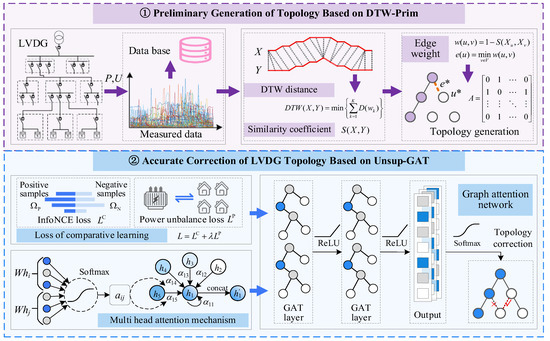
Figure 1. Architecture of the LVDG topology identification model based on Unsup-GAT.

2.2. Preliminary Construction Based on DTW-Prim Algorithm

2.2.1. Time Series Alignment and Low-Voltage Data Similarity Evaluation Based on DTW

When constructing the LVDG topology structure, voltage and current data can more directly reflect the electrical connection relationships between nodes. However, due to issues such as inconsistent data collection start times, varying data lengths, and time drift [27,28], the direct calculation of similarity will be greatly affected. To this end, a method for time series alignment and low-voltage data similarity evaluation based on DTW [26] is proposed, providing a basis for the identification and construction of the grid topology structure.

For two time series $X=\left\{x_1,x_2,\dots ,x_m\right\}$ and $Y=\left\{y_1,y_2,\dots ,y_n\right\}$ with lengths m and n, respectively, the distance metric between the elements of the two time series $d(x_i,y_j)$ is first defined as follows:

$$d(x_i,y_j)=\sqrt{{(x_i-y_j)}^2}$$

(1)

Furthermore, the other elements in the cumulative distance matrix are calculated using the recursive formula shown in Equation (2):

$$D(i,j)=d(x_i,y_j)+\min \left\{D(i-1,j),D(i,j-1),D(i-1,j-1)\right\}$$

(2)

where D denotes the cumulative distance matrix, which is used to store the minimum cumulative distance from the starting point (0,0) to the point (i,j), and $D(0,0)=0, D(i,0)=\infty , D(0,j)=\infty$.

After calculating the cumulative distance matrix D, the optimal path W from (m,n) back to (0,0) is found by backtracking the matrix D. The sum of all distances along the path is the minimum DTW distance:

$$DTW(X,Y)=\min \left\{{\displaystyle \sum _{k=1}^{K}D(w_k)}\right\}$$

(3)

$$NDTW(X,Y)={\displaystyle \frac{DTW(X,Y)}{\sqrt{mn}}}$$

(4)

where $DTW(X,Y)$ and $NDTW(X,Y)$ represent the DTW distance before and after normalization, respectively. w denotes a path obtained by backtracking from the cumulative distance matrix. $D(w_k)$ represents the distance between the elements of the two time series corresponding to the k-th point on path w. K is the total number of points on the optimal path.

Finally, the similarity coefficient between sequences X and Y is calculated based on Equation (5):

$$S(X,Y)=1-{\displaystyle \frac{NDTW(X,Y)-\underset{A,B\in \mathrm{\Omega },A\ne B}{\min }NDTW(A,B)}{\underset{A,B\in \mathrm{\Omega },A\ne B}{\max }NDTW(A,B)-\underset{A,B\in \mathrm{\Omega },A\ne B}{\min }NDTW(A,B)}}$$

(5)

where $S(X,Y)$ represents the similarity coefficient between sequences X and Y. $\mathrm{\Omega }$ denotes the set of all sequences.

2.2.2. Low-Voltage Topology Framework Generation Strategy Based on Prim Algorithm

After obtaining the sequence similarity coefficients of each node, the Prim algorithm is used to generate the low-voltage topology framework. Figure 2 shows a schematic diagram of topology generation based on the Prim algorithm, where the unconnected node with the maximum similarity coefficient to the already connected node set is selected in each iteration. The specific modeling process is as follows:

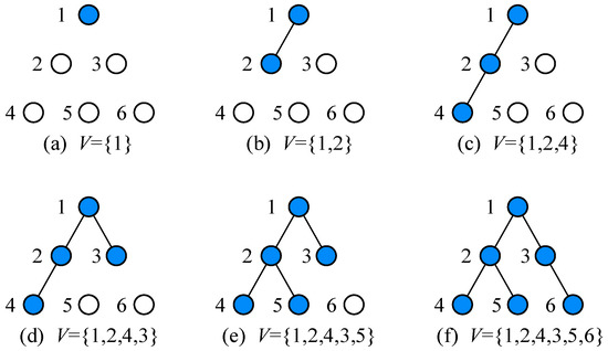
Figure 2. Schematic diagram of topology generation based on Prim algorithm.

Firstly, for all nodes to be identified, the low-voltage distribution transformer is selected as the root node r. Then, the already connected node set V = {r}, and the remaining nodes belong to the unconnected node set U. In addition, the edge set is initialized as an empty set $E_T=Ø$.

Secondly, for each unconnected node $u\in U$, the minimum weight edge $e(u)$ from u to the nodes in V is calculated:

$$e(u)=\underset{v\in V}{\min } w(u,v)$$

(6)

$$w(u,v)=1-S(X_u,X_v)$$

(7)

where $w(u,v)$ represents the weight of the edge $(u,v)$. $S(X_u,X_v)$ denotes the time series data similarity coefficient between node u and node v.

Then, the edge e* with the minimum weight among all $e(u)$ is selected, and the edge e* and the corresponding node u* are added to $E_T$ and V, respectively.

Finally, the above two steps are repeated until all nodes are connected, and the node adjacency topology relationship matrix A is output, as shown in Equation (8):

$$A=\left[\begin{array}{cccc}0& 1& \dots & 0\\ 1& 0& \dots & 1\\ ⋮& ⋮& \ddots & ⋮\\ 0& 1& \dots & 0\end{array}\right]$$

(8)

where $A_{ij}=1$ indicates that node i is connected to node j, otherwise, it indicates that they are not connected.

2.3. Precise Correction Based on Unsup-GAT Model

2.3.1. Feature Fusion Learning Based on Graph Attention Network

After obtaining the initial adjacency matrix A of the LVDG using the DTW and Prim algorithms, this paper adopts the GAT [29] to further mine the implicit correlation patterns between nodes. Through the attention mechanism, GAT can adaptively assign weights to different neighbor nodes, thereby more effectively capturing local and global topology information and improving the accuracy of topology correction.

To ensure that nodes retain their own features during information aggregation, an identity matrix is added to the adjacency matrix to ensure that all elements on its diagonal are 1.

$$A\prime =A+I$$

(9)

where $A\prime$ denotes the expanded adjacency matrix. I is the identity matrix.

Furthermore, symmetric normalization is performed on $A\prime$ to eliminate the feature scale difference caused by the difference in node degrees.

$$A″=D^{-\frac{1}{2}}A\prime D^{\frac{1}{2}}$$

(10)

where $A″$ represents the normalized adjacency matrix. D is the degree matrix of $A\prime$.

Subsequently, graph convolution is performed on the matrix $A″$ to obtain the output $H^{i+1}$ of each convolution layer.

$$H^{i+1}=\sigma (A″H^i{W}^i) ,i=0,1,\dots ,L$$

(11)

where $H^i$ denotes the output of the i-th convolution layer. $H^0=X$ is the input feature information and is the final output feature matrix. L is the number of graph convolution layers. $W^i$ is the weight coefficient of the i-th graph convolution layer.

Finally, the node features from multiple attention heads are concatenated to obtain the new feature vector of each node $h_i^{\prime }$, as shown in Equation (13):

$$h_i^{\prime }={\Vert }_{d=1}^D\sigma \left({\displaystyle \sum _{j\in {\mathcal{N}}_i}{\alpha }_{ij}^{\left(d\right)}{W}^{\left(d\right)}{h}_j}\right)$$

(12)

$${\alpha }_{ij}={\displaystyle \frac{\exp \left(\sigma \left(a^{\top }[W{h}_i\Vert W{h}_j]\right)\right)}{{\displaystyle \sum _{k\in {\mathcal{N}}_i}\exp }\left(\sigma \left(a^{\top }[W{h}_i\Vert W{h}_k]\right)\right)}}$$

(13)

where D is the number of attention heads. ${\mathcal{N}}_i$ denotes the set of neighbor nodes of node i. ${\alpha }_{ij}$ represents the attention weight coefficient between node i and node j. W is the weight parameter matrix. a is the learnable parameter. || denotes the concatenation operation. $\sigma (·)$ is the activation function.

The GAT model captures important correlation information in the graph topology through the multi-head attention mechanism, reduces the aggregation weight of irrelevant neighbors, and exhibits significant advantages in the task of precise low-voltage topology correction. In addition, GAT also has high robustness. Even when there is noisy data or inaccurate partial observation information, the model can still extract valuable information by reasonably assigning weights, ensuring the reliability of topology correction.

2.3.2. Loss Function Paradigm Based on Contrastive Learning

As an unsupervised learning paradigm, contrastive learning plays a unique role in the task of low-voltage topology correction, providing an effective solution to the problem of scarce sample data [30,31]. This paper considers both InfoNCE loss and physical constraint loss. By bringing the representations of positive samples (reasonable connections) closer and pushing the representations of negative samples (erroneous connections) further apart, the model is helped to implicitly learn topology rules, thereby correcting errors in the initial identification.

Comprehensively considering the DTW similarity coefficient and the known business data of power companies, the positive sample pairs and negative sample pairs can be constructed as shown in Equations (14) and (15), respectively:

$${\mathrm{\Omega }}_{\mathrm{P}}=\left\{(i,j)|S_{i,j}\ge {\theta }_{\mathrm{T}}\vee (i,j)\in {\mathrm{\Omega }}_{\mathrm{B}}\right\}$$

(14)

$${\mathrm{\Omega }}_{\mathrm{N}}=\left\{(i,j)|S_{i,j}\le {\theta }_{\mathrm{N}}\right\}$$

(15)

where ${\mathrm{\Omega }}_{\mathrm{P}}$ and ${\mathrm{\Omega }}_{\mathrm{N}}$ denote the positive sample pair set and negative sample pair set, respectively. $S_{i,j}$ is the DTW similarity coefficient between node i and node j. ${\theta }_{\mathrm{T}}$ and ${\theta }_{\mathrm{N}}$ are the thresholds for positive and negative sample pairs, respectively. ${\mathrm{\Omega }}_{\mathrm{B}}$ denotes the set of business data known to power companies (e.g., a certain branch box is connected to the distribution transformer).

The InfoNCE loss of the model $L^{\mathrm{C}}$ can be calculated using Equation (16):

$$L^{\mathrm{C}}={\displaystyle \frac{1}{N}}{\displaystyle \sum _{i=1}^N{L}_i^{\mathrm{C}}}$$

(16)

$$L_i^{\mathrm{C}}=-\log {\displaystyle \frac{\exp (sim(h_i^{\prime },h_{j^{+}}^{\prime })/\tau )}{\exp \left(sim(h_i^{\prime },h_{j^{+}}^{\prime })/\tau \right)+{\displaystyle \sum _{j^{-}\in {\mathcal{N}}_i^{-}}}\exp \left(sim(h_i^{\prime },h_{j^{-}}^{\prime })/\tau \right)}}$$

(17)

where $L_i^{\mathrm{C}}$ represents the InfoNCE loss of node i. N is the number of nodes. $j^{+}$ and $j^{-}$ are the positive and negative sample nodes corresponding to node i, respectively. ${\mathcal{N}}_i^{-}$ denotes the negative sample set corresponding to node i. $sim(h_i^{\prime },h_j^{\prime })$ represents the cosine similarity between the features of node i and node j. $\tau$ is the temperature parameter, which controls the sharpness of the distribution.

Furthermore, considering the physical principle of energy balance between the low-voltage distribution transformer and the users it supplies, it is ensured that the final topology identification result conforms to the law of energy conservation. Taking into account equipment measurement errors and line loss errors, the power between the transformer and the users it supplies should satisfy:

$$P_{k,t}^{\mathrm{T}}={\displaystyle \sum _{i\in {\mathrm{\Omega }}_k}{P}_{i,t}^{\mathrm{C}}}+{\epsilon }_t$$

(18)

where $P_{k,t}^{\mathrm{T}}$ represents the actual power value of transformer k at time t. $P_{i,t}^{\mathrm{U}}$ represents the power of user i at time t. ${\epsilon }_t$ is the error term. $i\in {\mathrm{\Omega }}_k$ denotes any user i supplied by transformer k.

Therefore, the loss term for violating power balance $L^{\mathrm{P}}$ is constructed as shown in Equation (19):

$$L^{\mathrm{P}}={\displaystyle \sum _{t=1}^T{\left[\mathrm{Re}\mathrm{LU}\left(\left|{\displaystyle \sum _{i\in {\mathrm{\Omega }}_k}{P}_{i,t}^{\mathrm{C}}}-P_{k,t}^{\mathrm{T}}\right|-{\epsilon }_t\right)\right]}^2}$$

(19)

where ReLU( ) is the Rectified Linear Unit.

Finally, the total loss function can be expressed as the weighted sum of the InfoNCE loss and the power imbalance loss:

$$L=L^{\mathrm{C}}+\lambda L^{\mathrm{P}}$$

(20)

where L is the total loss function. $\lambda$ is the weight parameter, which is used to control the influence degree of physical rules on model training.

By combining contrastive learning with physical constraint loss, the GAT model can fully utilize existing data and physical rules in an unsupervised environment, effectively correct erroneous connections in the low-voltage topology structure, and improve the accuracy and reliability of topology identification.

3. Algorithm Flow of the Proposed Two-Stage LVDG Topology Identification

Figure 3 shows the algorithm flow of the proposed LVDG topology identification based on contrastive learning. Firstly, the normalized DTW distance of the sample data is calculated based on the low-voltage measurement data, and the DTW similarity coefficient S(X,Y) is calculated using Equation (5). Secondly, the minimum weight edge $e(u)$ from node u to the nodes in V is calculated based on the Prim algorithm, and the edge e* and the corresponding node u* are added to $E_T$ and V, respectively, until all nodes are connected. Then, the identity matrix and symmetric normalization are added to the initial adjacency matrix A, and feature aggregation and learning are performed based on the multi-head attention mechanism. Finally, the positive and negative sample pair sets ${\mathrm{\Omega }}_{\mathrm{P}}$ and ${\mathrm{\Omega }}_{\mathrm{N}}$ are constructed based on Equations (14) and (15), and the total loss considering both InfoNCE loss and power imbalance loss is calculated based on Equation (20) to update the network parameters. The above steps are repeated until the maximum number of training epochs is reached, and the corrected LVDG topology identification result is output.

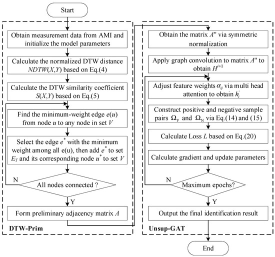
Figure 3. Flowchart of the proposed topology identification method based on contrastive learning.

4. Case Study Analysis

4.1. Case Configuration

Case studies are conducted on 7 LVDGs of different node scales in a certain region of China to verify the effectiveness of the proposed two-stage LVDG topology identification strategy based on contrastive learning. The data sampling interval is 15 min, and the time span ranges from 1 to 30 June 2024. The proportions of the training set, validation set, and test set are 80%, 10%, and 10%, respectively. The node scales of different LVDGs are shown in Table 1. The Unsup-GAT model has 2 hidden layers, with 128 units in each hidden layer, an output feature dimension of 32, a learning rate of 0.001, and the Adam optimizer is used. The computing environment configuration includes a CPU (i5-13600 kF), a GPU (RTX4070s), 32 GB of RAM, and the simulation platforms are Matlab 2023b and TensorFlow 2.12.0.

Table 1. Number of Nodes in Each LVDG.

	Number of Nodes
LVDG 1	49
LVDG 2	78
LVDG 3	31
LVDG 4	55
LVDG 5	51
LVDG 6	62
LVDG 7	86

To comprehensively reflect the performance of the proposed model, precision P, recall R, and F1 score F1) are adopted as performance evaluation indicators:

$$P={\displaystyle \frac{TP}{TP+FP}}$$

(21)

$$R={\displaystyle \frac{TP}{TP+FN}}$$

(22)

$$F_1={\displaystyle \frac{2\times P\times R}{P+R}}$$

(23)

where TP denotes the number of samples that are actually connected and predicted as connected. TN denotes the number of samples that are actually unconnected and predicted as unconnected. FP denotes the number of samples that are actually unconnected but predicted as connected. FN denotes the number of samples that are actually connected but predicted as unconnected.

4.2. Analysis of Model Training Process

Figure 4 shows the training loss curve of the proposed Unsup-GAT model over 1000 epochs. It can be seen from the figure that the value of the model loss function decreases rapidly with oscillations and tends to stabilize around 200 epochs. Specifically, in epochs 1–200, the model has weak ability to distinguish between positive and negative samples, and the attention weights are scattered, resulting in large fluctuations in the loss curve during this stage. Nevertheless, as the attention weights gradually focus on key neighbor nodes, the model begins to learn the local structural patterns in the graph, and the loss curve decreases rapidly. After 200 epochs, the model enters the stable optimization stage, and the training objective shifts from “rapid convergence” to “robust optimization”. Meanwhile, the loss value fluctuates slightly around 0.07. Through the refined adjustment of the attention mechanism and the dynamic balance of the self-supervised task, the model has captured the main feature distribution in the data, realizing the efficient capture of the essential features of LVDG topology identification.

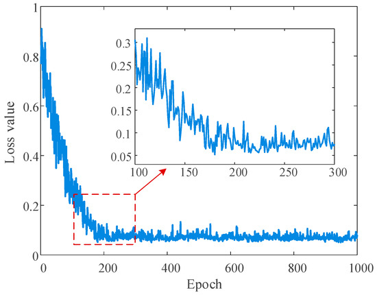
Figure 4. Training loss curve of the proposed Unsup-GAT model.

4.3. Analysis of Topology Identification Results

Table 2 and Figure 5 show the number of samples and evaluation indicators of the two-stage topology identification results, respectively. It can be seen from the topology identification results that in the Stage 1 topology identification, the performance of the model in different LVDGs shows certain differences. Specifically, the number of samples of LVDG 3 is relatively small, and the identification accuracy of positive and negative samples is acceptable from the data perspective. However, for LVDG 7 with a large number of topology nodes, there are certain deficiencies in the identification of positive samples, with relatively more misjudgments and omissions. The average F1 Score of the model in Stage 1 is 87.32%. After the correction identification in Stage 2, the performance of the model in all LVDGs is significantly improved. The average F1 Score of the model reaches 99.02%, which is 11.7 percentage points higher than the preliminary identification result in Stage 1. This indicates that the Unsup-GAT model proposed in Stage 2 can mine the implicit correlations of the LVDG topology, effectively improving the identification accuracy of positive and negative samples, and further reducing the number of misjudgments and omissions.

Table 2. Number of Topology Identification Samples for Different LVDGs.

	Stage 1 Results				Stage 2 Results
	TP	TN	FP	FN	TP	TN	FP	FN
LVDG 1	44	1161	15	4	48	1176	0	0
LVDG 2	73	2987	16	4	76	3001	2	1
LVDG 3	28	462	3	2	30	465	0	0
LVDG 4	51	1476	9	3	54	1485	0	0
LVDG 5	47	1267	8	3	49	1274	1	1
LVDG 6	55	1881	10	6	61	1891	0	0
LVDG 7	73	3637	18	12	83	3652	3	2

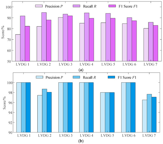
Figure 5. Topology identification indicator results of different LVDGs. (a) Indicator results of each LVDG after preliminary identification in Stage 1; (b) indicator results of each LVDG after correction identification in Stage 2.

Furthermore, Figure 6 and Figure 7 present the topological identification results and corresponding adjacency matrices for LVDG 3 and LVDG 6. It can be observed that the model has successfully identified the clear radial tree-like structures of LVDG 3 and LVDG 6 from the data. Specifically, for LVDG 3, with transformer node 1 as the root node, the model accurately identified a total of 10 branch box nodes, and precisely determined the connection relationships of 19 m box nodes numbered from 13 to 31. All the user nodes are correctly located at the outermost ends of the topology, and the entire network exhibits a well-defined hierarchical structure. This demonstrates that the proposed model has extremely high accuracy and practicality in topological structure reconstruction. Regarding the visualization results of the adjacency matrices, it is evident that the matrices display the typical sparse characteristics of tree-like topologies in graph theory, accurately reflecting the actual physical connection situations. This provides high-precision and visual data support for power supply companies in precise line loss analysis, rapid fault location, and scientific capacity expansion planning.

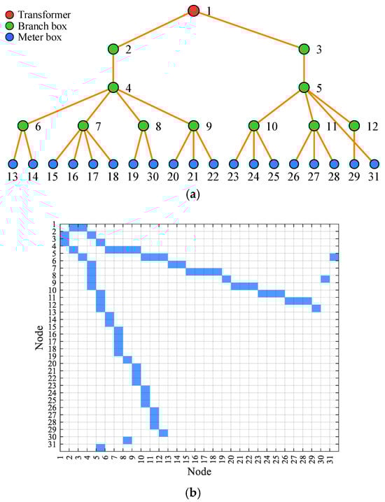
Figure 6. Topology result and adjacency matrix of LVDG 3. (a) Topology identification result of LVDG 3; (b) topology adjacency matrix of LVDG 3.

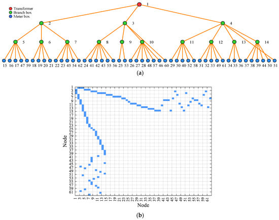
Figure 7. Topology result and adjacency matrix of LVDG 6. (a) Topology identification result of LVDG 6; (b) topology adjacency matrix of LVDG 6.

4.4. Comparison of Different Algorithms

To verify the superiority of the proposed topology identification algorithm, four algorithms are designed for simulation comparison:

Algorithm 1: Directly use the Euclidean distance as the weight and construct the topology structure based on the Prim algorithm.

Algorithm 2: Adopt the DTW algorithm for similarity evaluation and generate the topology based on the Prim algorithm (i.e., the Stage 1 DTW-Prim algorithm proposed in this paper).

Algorithm 3: On the basis of Algorithm 2, use the GAT model for correction identification.

Algorithm 4: The two-stage topology identification model proposed in this paper.

Algorithm 5: The graph learning-based method proposed in reference [25].

Algorithm 6: The K-means algorithm proposed in reference [9].

Figure 8 presents a comparison of the Precision, Recall, and F1 scores for the results obtained from the six algorithms, while Table 3 lists the accuracy metrics and computational time consumption for all six algorithms. As evident from Figure 8, the proposed Algorithm 4 excels in all three metrics, whereas Algorithm 1 and Algorithm 2 demonstrate relatively inferior identification results. Specifically, Algorithm 1 exhibits the poorest performance, primarily due to the inability of the Euclidean distance to directly capture the dynamic similarity between voltage time series. Algorithm 1 constructs a significant proportion of incorrect connection relationships, with an F1 score of only 82.97%, markedly lower than the other algorithms. Algorithm 2, leveraging DTW, overcomes the limitation of the Euclidean distance’s sensitivity to time series alignment, thereby generating a more accurate initial topology. Its Precision, Recall, and F1 scores are 83.17%, 92.04%, and 87.38%, respectively. The performance of Algorithm 3 further improves upon that of Algorithm 2. The introduction of the GAT correction module effectively enhances the Precision metric, indicating that the GAT model excels at learning and utilizing complex patterns within graph structures, enabling it to effectively identify and rectify local erroneous connections in the initial topology. Algorithm 5 demonstrates competitive performance, particularly in terms of Recall. This suggests that the graph learning approach is adept at capturing the overall connectivity patterns within LVDGs. However, its Precision is slightly lower compared to Algorithm 4. Algorithm 6 tends to group nodes based on their similarity in feature space without considering the underlying graph structure, leading to a high rate of incorrect connections. The performance indicators of Algorithm 4 are significantly higher than those of other comparison algorithms, with an F1 Score of 99.02%, which is 16.05 percentage points higher than that of Algorithm 1. In terms of computational time consumption, as listed in Table 3, Algorithm 1 is the fastest due to its simplicity and lack of training requirements. Algorithm 3 and Algorithm 4, involving the GAT model and two-stage topology construction process, require more computational time for training and inference but offer superior performance. Algorithm 6, despite its simplicity, does not offer any computational advantage over the more sophisticated algorithms in this context, as its performance is significantly inferior. The test results prove the effectiveness of the proposed two-stage topology identification algorithm and the superiority of its overall design.

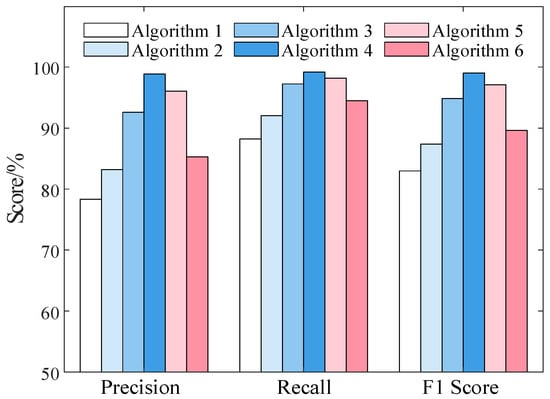
Figure 8. Comparison of Precision, Recall, and F1 Score among six algorithms.

Table 3. Comparison of accuracy index and calculation time of six algorithms.

	Precision/%	Recall/%	F1 Score/%	Training Duration/Min	Calculation Duration/s
Algorithm 1	78.33	88.20	82.97	/	1.55
Algorithm 2	83.17	92.04	87.38	/	3.71
Algorithm 3	92.58	97.23	94.85	86.50	3.82
Algorithm 4	98.85	99.19	99.02	97.25	3.80
Algorithm 5	96.05	98.18	97.10	102.08	3.15
Algorithm 6	85.27	94.47	89.63	/	4.29

4.5. Analysis of Model Robustness

Finally, to test the applicability and stability of the proposed algorithm in real complex environments, the performance of the six algorithms under different noise interferences is tested. In this study, Gaussian white noise with a mean of zero and variable amplitude is added to the original data to simulate the effects of factors such as measurement errors and communication interference, and the variation trend of the F1 Score of each algorithm is observed. The results are shown in Figure 9.

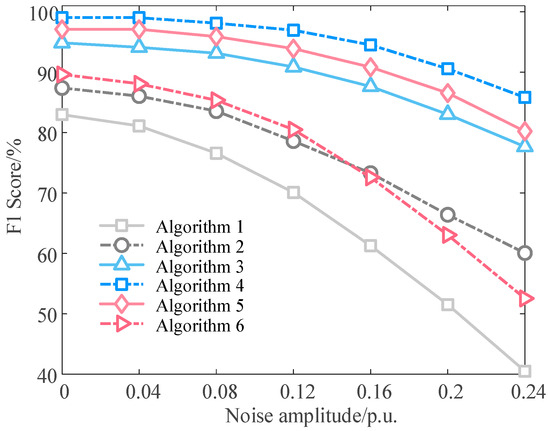
Figure 9. F1 Score of the six algorithms under different noise amplitudes.

To corroborate the differences in performance among the six algorithms, the Friedman test is applied to the F1 Scores of the six algorithms across different noise amplitudes. The null hypothesis of the Friedman test is that there is no significant difference in the robustness performance of the six algorithms. The test yielded a chi-squared statistic of 34.02, where p-value is much less than 0.05. This result indicates that we can reject the null hypothesis, and there are significant differences in the performance of the six algorithms. Furthermore, it can be seen from Figure 9 that with the increase in noise amplitude, the performance of all algorithms shows a downward trend, but the proposed algorithm exhibits significant robustness advantages. Specifically, the F1 Scores of Algorithm 1 and Algorithm 6 decline sharply as noise increases. For Algorithm 1, with every 0.04 p.u. increase in noise amplitude, its F1 Score decreases by an average of 7.08 percentage points. This implies that even minor noise interference can lead to inaccurate distance calculations, making it difficult to apply in practical engineering. By finding the optimal alignment path, Algorithm 2 can effectively cope with slight jitters on the time axis and random disturbances in amplitude, resulting in improved model robustness. Algorithm 3 performs well under low noise conditions, but its gain is limited under high noise conditions. The proposed Algorithm 4 maintains the highest performance throughout the entire noise range. For every 0.04 p.u. increase in noise amplitude, its F1 Score decreases by an average of only 2.2 percentage points. This is mainly due to the effective cascaded anti-noise mechanism formed by the two-stage design: Stage 1 first filters out the interference of most random noise and provides a topology with a roughly correct structure where “noise has been partially suppressed”. Stage 2 then uses the knowledge learned through data-driven methods to perform more precise secondary denoising and error correction. The robustness test shows that compared with other comparison algorithms, the proposed algorithm not only has the highest accuracy but also can better adapt to the real LVDG environment.

5. Conclusions

This paper proposes a novel two-stage topology identification strategy for LVDGs based on contrastive learning. The DTW and Prim algorithms are used for the preliminary construction of the LVDG topology, and a GAT model based on the contrastive learning paradigm is used to mine the implicit correlation patterns between nodes and output the corrected identification result. Through case experiments conducted on 7 station areas of different scales, the following conclusions are drawn:

(1)

The proposed DTW-Prim algorithm can accurately capture the similarity relationships between nodes through the elastic alignment and similarity quantification of time series, and construct the initial topology structure. Experiments on 7 LVDGs of different scales show that the average F1 Score of the preliminary identification result in Stage 1 reaches 87.32%, laying a topological foundation for the precise correction in Stage 2.

(2)

The proposed Unsup-GAT model based on the contrastive learning paradigm realizes the learning of complex correlation patterns in unsupervised scenarios through node information aggregation and attention weight assignment, and can identify and correct local connection errors in the initial topology. Experimental results show that the average F1 Score of the topology identification result in Stage 2 is increased by 11.7 percentage points, finally reaching 99.02%.

(3)

The robustness test shows that compared with other comparison algorithms, the proposed algorithm not only has the highest accuracy but also can realize highly robust inference of the topology structure through the progressive framework of “preliminary construction-precise correction”. For every 0.04 p.u. increase in noise amplitude, the F1 Score of the proposed algorithm decreases by an average of only 2.2 percentage points, which verifies the identification performance of the proposed algorithm in practical engineering scenarios with poor data quality.

Future research will focus on integrating large-scale, high-dimensional real-time monitoring information into the topology identification process. Meanwhile, we will delve into parameter optimization and explore how to safeguard the method against security attacks [32,33], so as to enhance its adaptability to dynamic topology changes.

References

- Rizeakos, V.; Bachoumis, A.; Andriopoulos, N.; Birbas, M.; Birbas, A. Deep learning-based application for fault location identification and type classification in active distribution grids. Appl. Energy 2023, 338, 120932. [Google Scholar] [CrossRef]
- García, S.; Mora-Merchán, J.M.; Larios, D.F.; Personal, E.; Parejo, A.; León, C. Phase topology identification in low-voltage distribution networks: A Bayesian approach. Int. J. Electr. Power Energy Syst. 2023, 144, 108525. [Google Scholar] [CrossRef]
- Lei, Y.; Yang, F.; Feng, Y.; Hu, W.; Cheng, Y. A Topology Identification Strategy of Low-Voltage Distribution Grids Based on Feature-Enhanced Graph Attention Network. Energies 2025, 18, 2821. [Google Scholar] [CrossRef]
- Athanasiadis, C.L.; Papadopoulos, T.A.; Kryonidis, G.C.; Doukas, D.I. A review of distribution network applications based on smart meter data analytics. Renew. Sustain. Energy Rev. 2024, 191, 114151. [Google Scholar] [CrossRef]
- Zhao, J.; Xu, M.; Wang, X.; Zhu, J.; Xuan, Y.; Sun, Z. Data-driven based low-voltage distribution system transformer-customer relationship identification. IEEE Trans. Power Deliv. 2021, 37, 2966–2977. [Google Scholar] [CrossRef]
- Byun, H.J.; Zheng, Y.P.; Choi, S.J.; Shon, S.G. New identification method for power transformer and phase in distribution systems. Appl. Mech. Mater. 2018, 878, 291–295. [Google Scholar] [CrossRef]
- Ge, H.; Xu, B.; Zhang, X.; Bi, Y. Low-voltage overhead lines topology identification method based on high-frequency signal injection. Arch. Electr. Eng. 2021, 70, 791–800. [Google Scholar] [CrossRef]
- García, S.; Fresia, M.; Mora-Merchán, J.M.; Carrasco, A.; Personal, E.; Leon, C. A data-driven topology identification method for low-voltage distribution networks based on the wavelet transform. Electr. Power Syst. Res. 2025, 243, 111517. [Google Scholar] [CrossRef]
- Al Khafaf, N.; Song, H.; McGrath, B.; Jalili, M. Identification of low voltage distribution transformer–customer connectivity based on unsupervised learning. Energy Rep. 2023, 9, 72–79. [Google Scholar] [CrossRef]
- Jiao, F.; Li, Z.; Ai, J.; Yang, H.; Deng, Y.; Li, D.; Gao, W.; Lai, Z.; Fu, X. Topology Identification Method for Low-Voltage Distribution Node Networks Based on Density Clustering Using Smart Meter Real-time Measurement Data. IEEE Access 2024, 12, 83600–83610. [Google Scholar] [CrossRef]
- Feng, N.; Du, Y.; Ding, Y. A heuristic-search-based topology identification and parameter estimation method in low voltage distribution grids with low observability. IEEE Trans. Smart Grid 2024, 15, 5826–5839. [Google Scholar] [CrossRef]
- Zhao, J.; Li, L.; Xu, Z.; Wang, X.; Wang, H.; Shao, X. Full-scale distribution system topology identification using Markov random field. IEEE Trans. Smart Grid 2020, 11, 4714–4726. [Google Scholar] [CrossRef]
- Zhang, H.; Cao, J.; Shen, Q. Topology identification of low-voltage distribution network based on latent tree model and cluster search. J. Electr. Power Sci. Technol. 2025, 40, 170–178, 195. [Google Scholar]
- Zhang, L.; Cong, W.; Dong, G.; Sun, Y. Method for single-phase electric meter phase discrimination based on multiple linear regression. In Proceedings of the 2019 IEEE 8th International Conference on Advanced Power System Automation and Protection (APAP), Xi’an, China, 21–24 October 2019; IEEE: Piscataway, NJ, USA, 2019; pp. 177–181. [Google Scholar]
- Liu, B.; Chen, J.; Li, J. Distribution network topology identification method based on state estimation with mixed integer programming and structural equation model. Int. J. Electr. Power Energy Syst. 2024, 162, 110251. [Google Scholar] [CrossRef]
- Tian, Z.; Wu, W.; Zhang, B. A mixed integer quadratic programming model for topology identification in distribution network. IEEE Trans. Power Syst. 2015, 31, 823–824. [Google Scholar] [CrossRef]
- Farajollahi, M.; Shahsavari, A.; Mohsenian-Rad, H. Topology identification in distribution systems using line current sensors: An MILP approach. IEEE Trans. Smart Grid 2019, 11, 1159–1170. [Google Scholar] [CrossRef]
- Karimi, H.S.; Natarajan, B. Joint topology identification and state estimation in unobservable distribution grids. IEEE Trans. Smart Grid 2021, 12, 5299–5309. [Google Scholar] [CrossRef]
- Ma, L.; Wang, L.; Liu, Z. Topology identification of distribution networks using a split-EM based data-driven approach. IEEE Trans. Power Syst. 2021, 37, 2019–2031. [Google Scholar] [CrossRef]
- Razmi, P.; Ghaemi Asl, M.; Canarella, G.; Emami, A.S. Topology identification in distribution system via machine learning algorithms. PLoS ONE 2021, 16, e0252436. [Google Scholar] [CrossRef]
- Xu, D.; Wu, Z.; Xu, J.; Hu, Q. A data-model hybrid driven topology identification framework for distribution networks. CSEE J. Power Energy Syst. 2023, 10, 1478–1490. [Google Scholar]
- Wu, H.; Xu, Z.; Zhao, J.; Chai, S. Gridtopo-GAN for distribution system topology identification. IEEE Trans. Ind. Inform. 2022, 19, 5356–5366. [Google Scholar] [CrossRef]
- Ni, Q.; Jiang, H. Topology identification of low-voltage distribution network based on deep convolutional time-series clustering. Energies 2023, 16, 4274. [Google Scholar] [CrossRef]
- Poudel, S.; Ramachandran, T.; Veeramany, A.; Francis, C.; Reiman, A.P. Topology Identification Using Graph Theory Informed State Estimation-Based Model Selection for Power Distribution Systems. IEEE Trans. Ind. Inform. 2023, 20, 3563–3573. [Google Scholar] [CrossRef]
- Flynn, C.; Pengwah, A.B.; Razzaghi, R.; Andrew, L.L.H.; Flynn, D. An improved algorithm for topology identification of distribution networks using smart meter data and its application for fault detection. IEEE Trans. Smart Grid 2023, 14, 3850–3861. [Google Scholar] [CrossRef]
- Senin, P. Dynamic time warping algorithm review. Inf. Comput. Sci. Dep. Univ. Hawaii Manoa Honol. USA 2008, 855, 40. [Google Scholar]
- Zhang, S.; Liu, W.; Wan, H.; Bai, Y.; Yang, Y.; Ma, Y.; Lu, Y. Combing data-driven and model-driven methods for high proportion renewable energy distribution network reliability evaluation. Int. J. Electr. Power Energy Syst. 2023, 149, 108941. [Google Scholar] [CrossRef]
- Barja-Martinez, S.; Aragüés-Peñalba, M.; Munné-Collado, Í.; Lloret-Gallego, P.; Bullich-Massagué, E.; Villafafila-Robles, R. Artificial intelligence techniques for enabling Big Data services in distribution networks: A review. Renew. Sustain. Energy Rev. 2021, 150, 111459. [Google Scholar] [CrossRef]
- Veličković, P.; Cucurull, G.; Casanova, A.; Romero, A.; Lio, P.; Bengio, Y. Graph attention networks. arXiv 2017, arXiv:1710.10903. [Google Scholar]
- Tian, Y.; Sun, C.; Poole, B.; Krishnan, D.; Schmid, C.; Isola, P. What makes for good views for contrastive learning? Adv. Neural Inf. Process. Syst. 2020, 33, 6827–6839. [Google Scholar]
- Khosla, P.; Teterwak, P.; Wang, C.; Sarna, A.; Tian, Y.; Isola, P.; Maschinot, A.; Liu, C.; Krishnan, D. Supervised contrastive learning. Adv. Neural Inf. Process. Syst. 2020, 33, 18661–18673. [Google Scholar]
- Habib, A.K.M.A.; Hasan, M.K.; Hassan, R.; Islam, S.; Thakkar, R.; Vo, N. Distributed denial-of-service attack detection for smart grid wide area measurement system: A hybrid machine learning technique. Energy Rep. 2023, 9, 638–646. [Google Scholar] [CrossRef]
- Yang, L.; Teh, J. Review on vulnerability analysis of power distribution network. Electr. Power Syst. Res. 2023, 224, 109741. [Google Scholar] [CrossRef]
Disclaimer/Publisher’s Note: The statements, opinions and data contained in all publications are solely those of the individual author(s) and contributor(s) and not of MDPI and/or the editor(s). MDPI and/or the editor(s) disclaim responsibility for any injury to people or property resulting from any ideas, methods, instructions or products referred to in the content. |
© 2025 by the authors. Licensee MDPI, Basel, Switzerland. This article is an open access article distributed under the terms and conditions of the Creative Commons Attribution (CC BY) license (https://creativecommons.org/licenses/by/4.0/).