Abstract
To address the problem of uncoordinated operation between distributed generation (DG) inverters and dedicated power quality devices, this paper proposes a coordinated optimization model for harmonic and voltage compensation in microgrids. The model considers the capacity constraints of DG inverters and compensation devices, aiming to realize efficient utilization of multi-resource compensation capabilities. A dual-objective optimization framework is established, which simultaneously minimizes total economic cost and enhances overall power quality performance. The first objective function reflects investment and operational costs, while the second quantifies system performance through total harmonic distortion (THD) and average voltage deviation (AVD). The Normal–Normal Constraint (NNC) method is adopted to ensure optimization stability and feasible trade-offs between the two objectives. The proposed approach is validated on the IEEE 33-bus microgrid system, and its results are compared with traditional heuristic algorithms such as PSO. Simulation results show that the proposed method effectively reduces total operating cost while significantly improving harmonic and voltage compensation performance. This study provides a practical reference for coordinated power quality management in microgrids.
1. Introduction
To alleviate the energy crisis and reduce environmental pollution, distributed generation (DG) is being increasingly integrated into microgrids, driving the rapid emergence of a “dual-high” trend characterized by high DG penetration and a growing presence of power electronic devices [1,2,3]. However, the large-scale deployment of DG introduces a substantial number of power electronic interfaces into the microgrids, resulting in more severe harmonic pollution. This problem becomes particularly significant when DG operates under low-power conditions, where harmonic distortion tends to increase [4]. Moreover, a growing number of nonlinear loads are being integrated into microgrids via power electronic converters, which inevitably inject harmonic currents into the system and further deteriorate power quality. In addition, due to environmental variations such as solar radiation and temperature, the inherently random and intermittent output of distributed generation (DG) further intensifies voltage instability and deviations in microgrids [5]. Therefore, effective power quality management has become increasingly urgent to ensure the safe and reliable operation of microgrids.
With the continuous advancement of power electronics technology, modern power quality management equipment has been evolving toward greater diversity, multi-functionality, proactivity, and integration. For instance, harmonic mitigation devices have gradually developed from traditional passive filters to active power filters (APFs). In addition to effectively suppressing harmonic distortions, APFs are also capable of compensating reactive power and addressing issues such as three-phase imbalance [6,7], thereby providing a more comprehensive and efficient solution to power quality problems. Reactive power compensation is primarily achieved using devices such as the Dynamic Voltage Restorer (DVR) [8], the Static Var Compensator (SVC) [9], and the Static Var Generator (SVG) [10]. In addition to dedicated power quality control devices, certain multifunctional equipment can also enhance power quality. For example, conventional DG grid-connected inverters, while primarily designed for active power delivery, can regulate voltage by controlling reactive power. Moreover, advanced multifunctional inverters provide additional capabilities such as harmonic suppression [11], reactive power compensation [12], and mitigation of three-phase imbalances [13]. These advancements demonstrate that modern power quality management devices are highly diverse in both types and functionalities. By effectively utilizing existing devices and coordinating the mitigation of power quality issues, including harmonics and voltage fluctuations, in line with the requirements of microgrids, the utilization of resources can be optimized and the overall efficiency of equipment can be enhanced.
Indeed, extensive studies have been carried out worldwide to tackle power quality issues, with particular emphasis on harmonic mitigation and voltage deviation control. In the field of harmonic mitigation, ref. [14] adopts an enhanced ant colony-based mixed-integer distributed optimization approach to address the multi-objective parameter design problem of single-tuned passive filters, ensuring that the quality factor of the filter stays within the prescribed limits and preventing the occurrence of harmonic resonance. In [15], the particle swarm optimization (PSO) algorithm is utilized to minimize the total harmonic distortion (THD) of the grid-side current while enhancing the utilization efficiency of the shunt active power filter (SAPF) capacity. In the field of voltage deviation control, ref. [16] introduces a multi-objective model for reactive power and voltage regulation based on an entropy-weighted grey wolf optimization algorithm, effectively improving node voltage quality and system stability. In ref. [17], a coordinated active and reactive power optimization approach is proposed for microgrids, in which an improved particle swarm optimization algorithm determines the optimal placement and sizing of SVCs to minimize operating costs, mitigate voltage variations, and enhance PV integration capability. In addition, DG grid-connected inverters have also been utilized to improve power quality. Ref. [18] proposes an optimal operation method for active distribution networks that leverages DG inverters for unbalance and harmonic compensation, employing a semidefinite programming-based optimization model to minimize power losses, harmonic distortion, and voltage unbalance. However, the aforementioned studies primarily target a single type of power quality issue and optimize the configuration of the corresponding mitigation device, without considering the coordinated utilization of multiple mitigation resources (such as DG inverters and dedicated compensation devices) to comprehensively address various power quality problems.
In summary, existing studies have rarely considered the coordinated control between DG grid-connected inverters and dedicated power quality devices. To address this gap, this paper proposes an integrated optimization framework that achieves multi-resource coordination for harmonic and voltage mitigation in microgrids. The main contributions of this work are summarized as follows:
(1) A comprehensive optimization model is established to jointly schedule DG inverters and dedicated compensators for harmonic and voltage regulation. The model explicitly captures the coupling and coordination among the active, reactive, and harmonic compensation capacities within DG inverters, ensuring coordinated utilization of multiple mitigation resources.
(2) A dual-objective formulation is developed to balance economic cost and power quality performance. The Normal–Normal Constraint (NNC) method is introduced to enhance optimization stability and ensure physically feasible trade-offs between investment cost and system performance.
(3) The proposed method is verified on the IEEE 33-bus microgrid system and compared with traditional heuristic algorithms such as PSO. Simulation results demonstrate that the proposed approach effectively reduces total operating cost while significantly enhancing the overall power quality mitigation performance, achieving coordinated improvement in both economic efficiency and technical quality.
2. Power Quality Management Functions of Grid-Connected Inverter in Microgrid
In distributed generation (DG) systems, the grid-connected inverter (GCI) functions as a vital power conversion interface that converts DC from energy sources into AC suitable for grid integration, thereby serving as a fundamental component of microgrids. The operational configuration of a typical GCI is illustrated in Figure 1. With the continuous evolution of power electronic technologies, GCIs have extended their functionality beyond mere energy conversion to encompass reactive power support and harmonic mitigation, contributing significantly to power quality enhancement. Nevertheless, the inverter’s compensation capability is inherently restricted by the predicted active power and current, as defined in Equations (1) and (2).
where and denote the active power corresponding to the fundamental and h-order harmonic components of the DG unit; is the predicted active power of the DG; and correspond to the current associated with the fundamental frequency and the h-th harmonic components of the GCI; denotes the maximum allowable current of the GCI; corresponds to the fundamental voltage measured at the point of common coupling of the GCI; H is the maximum harmonic order; k corresponds to the harmonic current compensation margin of the GCI.
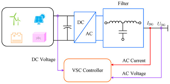
Figure 1.
Grid connection principle of typical DG.
The GCI generally supplies both active and reactive power to the grid through a feeder line, which can be mathematically represented by the following equations:
where corresponds to the fundamental voltage at the feeder line connecting the GCI to the grid; X denotes the equivalent reactance between the GCI and the feeder line; is the phase angle difference between the GCI grid-side voltage and the feeder-side voltage.
It should be noted that Equations (3) and (4) are derived under the simplifying assumption , which is reasonable for medium-voltage feeders. However, in low-voltage microgrids where may approach unity, the full R–X power–flow relations (see Equations (9)–(11)) are used in the optimization and simulation to ensure accuracy.
To maintain the reliable and stable operation of the GCI, both the grid-side voltage magnitude and the phase angle should be kept within their permissible limits
where and denote the lower and upper bounds of the fundamental voltage of the GCI, respectively; correspond to the minimum and maximum allowable values of the phase angle , respectively.
The fundamental reactive power should satisfy the following relationship:
3. Optimization Model of the Microgrids Considering GCI Compensation
3.1. Objective Function
The developed multi-objective optimization model aims to simultaneously enhance power quality and reduce compensation cost by establishing an optimal balance between the two objectives.
where is the total cost of power quality management, is a quantitative measure of power quality in active microgrids; , , and represent the installation cost of the SAPF, the investment cost per unit of compensating capacity, the operation and maintenance cost of the compensating device, and the penalty coefficient for violating harmonic distortion limits, respectively; is the number of SAPF; is the rated capacity of the ith SAPF; is the actual compensating capacity of the ith SAPF at time t; is the total harmonic voltage distortion exceeding allowable limits across all nodes and time periods; T is set to 24; n represents the total number of nodes in the system; is a weighting coefficient reflecting the relative importance of harmonic mitigation; corresponds to the voltage harmonic distortion measured at node i at time t; corresponds to the voltage deviation of node i at time t.
3.2. Constraints
3.2.1. Fundamental Power Flow Constraint
3.2.2. Harmonic Power Flow Constraint
The expression for the harmonic current of the load is derived as follows:
where represents the coupling admittance between the h-th harmonic current and k-th harmonic voltage of the load; represents the k-th harmonic voltage at node i and time t.
3.2.3. SAPF Capacity Constraints
The compensation capacity of each SAPF should remain within its rated limit:
where denotes the reactive compensation current capacity of the SAPF at node i and time t, the unit of is A; denotes the harmonic current compensation capacity of the SAPF at node i and time t; denotes the maximum rated current capacity of the SAPF; and correspond to the lower and upper boundaries of the SAPF compensation capacity, respectively.
3.2.4. Node Voltage Magnitude Constraint
The voltage magnitude at node i and time t is subject to the following operational constraint:
where and represent the minimum and maximum node voltage limits, respectively.
3.2.5. Harmonic Voltage Distortion Rate Constraint
The total harmonic distortion of the voltage is required to meet the following constraint:
3.3. Multi-Objective Optimization Utilizing the NNC Approach
3.3.1. Solution Methods for Multi-Objective Optimization Problems
The mathematical representation of a general multi-objective optimization problem is given as follows:
where is the objective function of the optimization model, , d is the number of decision variables; is the number of objective functions; and are the inequality and equality constraints in the optimization model, respectively; p and v correspond to the numbers of inequality and equality constraint functions, respectively.
Unlike single-objective optimization problems, the multi-objective optimization problem investigated in this paper does not yield a unique global optimum. Rather, it produces a set of Pareto-optimal solutions that collectively form the Pareto front in the objective space. For the specific two-objective optimization case addressed herein, the Pareto front usually takes the form of a curve. In general, existing methods for solving multi-objective optimization problems can be broadly divided into vector approaches and scalarization approaches.
Vector-based approaches generally employ artificial intelligence algorithms—such as multi-objective particle swarm optimization and multi-objective genetic algorithms—to obtain the Pareto-optimal solution set. Despite their flexibility and effectiveness, these methods often face limitations in large-scale power system applications due to their significant computational demands and extended convergence times.
Scalar-based methods reformulate multi-objective optimization problems into equivalent single-objective formulations through appropriate transformation techniques, thereby facilitating the generation of representative Pareto-optimal solutions. Among these, the normalized normal constraint (NNC) method is particularly effective, as it produces uniformly distributed Pareto fronts and demonstrates strong robustness in handling non-convex problems, reducing the likelihood of convergence to local optima. Therefore, the NNC method is adopted in this study to solve the proposed multi-objective optimization model.
3.3.2. Implementation Steps of the NNC Method
For an N-dimensional multi-objective optimization problem, the NNC method reduces the feasible space and transforms the problem into a set of single-objective subproblems. This approach generates a uniformly distributed Pareto solution set within the feasible region, offering decision-makers a diverse set of configuration options across different performance trade-offs. In addition, the method features a relatively simple implementation.
The detailed procedure of the NNC method is given as follows:
Step 1: Decompose the multi-objective configuration model established in Section 3.1 into two single-objective optimization models, and solve each one separately to obtain its corresponding optimal solution and .
Step 2: To eliminate the influence of different units, the two single-objective functions are normalized based on Equation (19). Using the optimal solutions derived in Step 1, denoted as points and , a utopia line is subsequently constructed, with its direction vector defined accordingly , as shown in Figure 2.
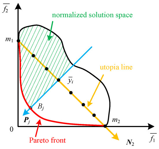
Figure 2.
Normalized solution space for the multi-objectives optimization problems.
Step 3: Divide the utopia line into y equal segments, generating evenly spaced points.
Step 4: At each division point on the utopia line, a normal line is constructed, which intersects the Pareto front at point . Here, and denote the vectors from the origin to the points and , respectively. To identify the corresponding point on the Pareto front, a new single-objective optimization model is formulated based on Equation (20).
where and represent th0e equality and inequality constraints of the model, respectively.
After the introduction of the inequality , the solution space of the newly formulated single-objective optimization model is constrained to the upper region illustrated in Figure 2. By solving the model at each division point, a uniformly distributed set of Pareto-optimal solutions can be obtained. The single-objective optimization model is solved using the Human Evolution Optimization Algorithm (HEOA) reported in [19]. Compared with classical algorithms such as Particle Swarm Optimization (PSO), the Genetic Algorithm (GA), and Differential Evolution (DE), the HEOA demonstrates stronger adaptability and search efficiency. By simulating human learning, self-improvement, and cooperative decision-making, HEOA dynamically balances exploration and exploitation, effectively avoiding premature convergence and maintaining population diversity. Its adaptive learning mechanism allows individuals to share and refine knowledge throughout the evolution process, leading to faster convergence and more accurate solutions. Moreover, the inherent flexibility of HEOA enables it to be easily extended to multi-objective optimization, where its collaborative learning and adaptive strategies help maintain a well-distributed set of Pareto-optimal solutions with improved convergence and diversity. The detailed comparative study of the algorithms will be discussed in Section 3.2. The detailed description of the algorithm is given as follows:
(1) Initialization Stage
The HEOA begins with a chaotic population initialization to enhance the uniformity and ergodicity of the search space. A logistic chaotic map with control parameter is adopted to generate a non-repetitive sequence:
where ∈ [0, 1] denotes the i-th chaotic sequence value, and ∈ [3.7, 4.0] is the chaotic control parameter ensuring complete chaos. The initial positions of individuals are mapped into the search domain by the following:
where and are the lower and upper bounds of each dimension, respectively, and represents the initial position of an individual.
(2) Exploration Stage
After the population is initialized, the subsequent step involves evaluating the fitness of each candidate solution. In the experimental setup, the exploration stage was defined as the first one-fourth of the total number of iterations. During the early stages of human development, when individuals encounter unfamiliar environments with limited prior knowledge, they typically employ a uniform exploration strategy. This behavior can be formulated mathematically as expressed in Equation (23).
where and are the current and updated positions of the i-th individual; is the adaptive function; t is the current number of iterations; is the maximum iterations; is the best-know position so far; is the population mean position; is the dimensionality of the question; is the distribution; is the jump factor that scales the exploration step; floor() represents the floor operation, which performs rounding down to the nearest integer; denotes the jump coefficient; is a random number, which is in the range of [0, 1].
The detailed formulations of , adaptive function , distribution and jumping strategy can be found in [19].
(3) Human development Stage
In the human development stage, the HEOA divides the population into four social roles, namely leaders, explorers, followers, and losers. This stage imitates cooperative human learning and adaptive behavior, where each group follows a distinct update strategy that jointly maintains a balance between exploration and exploitation.
Leaders represent the top 40% of individuals with superior adaptability. Their actions alternate between local refinement and global exploration depending on the environmental complexity, which is controlled by a threshold, :
where follows a normal distribution and is a random complexity factor. The adaptive knowledge acquisition coefficient gradually decreases with iterations according to
where is the learning rate.
Explorers, representing 40% to 80% of the population, are responsible for searching uncharted regions and maintaining population diversity. Their position update rule is defined as
where denotes the position of the least adapted individual. This mechanism helps individuals move away from low-quality regions and promotes global exploration.
Followers, which account for 80% to 90% of the population, imitate superior individuals to accelerate convergence while maintaining diversity. Their behavior is modeled as
where represents a randomly selected dimension index. This mechanism allows followers to selectively learn from better-performing individuals and enhances convergence stability.
The remaining 10% of the population are defined as losers and are replaced through an elitist regeneration process to sustain evolutionary dynamics. The update rule is formulated as
3.3.3. Final Decision Scheme Selection
After obtaining a series of uniformly distributed Pareto solutions, the decision-maker can select, from the Pareto solution set, a compromise solution that achieves relatively balanced performance across multiple objectives by the system’s operational requirements. In this study, the final optimal configuration scheme is determined by calculating the weighted Euclidean distance of each Pareto solution to the ideal point. The specific procedure is as follows:
Step 1: Apply the NNC method to solve the multi-objective optimization configuration model and obtain a set of uniformly distributed Pareto solutions;
Step 2: Identify the ideal point and the nadir point for each objective function in the Pareto solution set, and compute the normalized value of each solution for every objective using the interval scaling formula;
where is the minimum value of the k-th objective for solution in the Pareto set; is the maximum value of the k-th objective for solution in the Pareto set; is the value of the i-th solution on the k-th objective; denotes the normalized deviation value of the i-th solution on the k-th objective.
Step 3: Define the weight vector for the objectives according to the decision-making requirements as , and normalize it to satisfy the expression as follows:
where is the weight of the j-th objective.
Step 4: Calculate the weighted Euclidean distance from each Pareto solution to the ideal point as follows:
where denotes the distance of the i-th solution.
Step 5: Rank the Pareto solutions according to their computed distance values, and select the solution with the smallest distance as the compromise solution under the weighted Euclidean metric.
4. Case Study
4.1. Optimization Model Solving
To evaluate the effectiveness and applicability of the proposed optimization model, a case study is conducted on the IEEE 33-bus system. DGs with a rated capacity of 30 MW are installed at buses 12, 18, 25, 29, and 33, as shown in Figure 3. Figure 4 illustrates the 24 h active power output profiles of the five DG units. Specifically, and denote the active power outputs of the wind turbine units connected at nodes 12 and 18, respectively, while , and represent those of the photovoltaic units connected at nodes 25, 29, and 33, respectively. Each DG is connected through a grid-connected inverter that provides harmonic mitigation and voltage regulation, thereby enabling coordinated power quality improvement in conjunction with an SAPF. A 24 h operating scenario based on the DG output and load profiles of a representative urban district is used to determine the optimal placement and sizing of the SAPF. The line and load parameters of the 33-bus system are adopted from [20]. Bus 1 operates at a voltage level of 12.66 kV, which is stepped down to 380 V through the main transformer, resulting in a voltage level of 380 V for buses 2 through 33. The population size is set to 100 and the maximum number of iterations is 300. The remaining parameters are configured as follows: is set to 0.5, representing an equal weighting between harmonic suppresion and voltage regulation; the values of , , and are 3000, 360, 10 and 500,000, respectively. Furthermore, the maximum limits of voltage deviation and harmonic voltage distortion rate in the microgrids are set to 3% and 4%, respectively. In this study, the parameters of the HEOA are set as follows: , , , , , . The definitions of parameters , , and A can be found in [19]. The logistic control coefficient () ensures fully chaotic initialization for population diversity. The initial exploration weight () and knowledge coefficient () regulate the adaptive learning and exploration intensity during iterations. The levy parameters ( and ) control the frequency and scale of random jumps, facilitating global search capability. The scenario threshold (A = 0.6) maintains stability in decision-making.
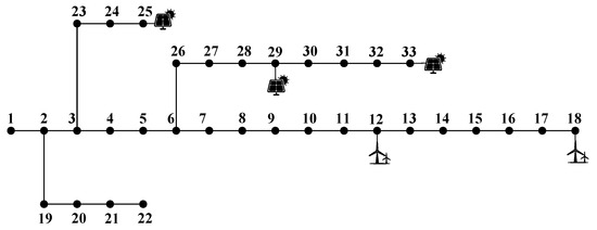
Figure 3.
Topology of the IEEE 33-bus system integrated with renewable energy sources.
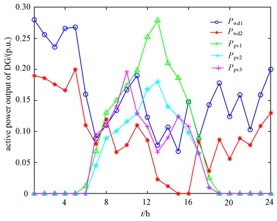
Figure 4.
The 24 h active power output profiles of the DG units.
This paper focuses on the mitigation of the 5th, 7th, 11th, 13th, and 17th harmonics. Based on the harmonic equivalent model of DG presented in [21], harmonic currents of the 5th, 7th, 11th, 13th, and 17th orders are injected at the DG access node. By performing fundamental power flow and harmonic power flow calculations, the voltage and total harmonic distortion of voltage at each node of the microgrids before mitigation are obtained, as shown in Figure 5 and Figure 6.
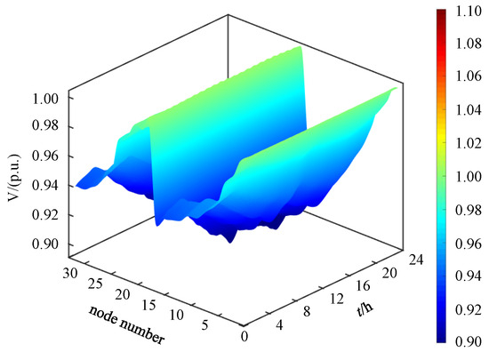
Figure 5.
Voltage distribution of all buses over 24 h before mitigation.
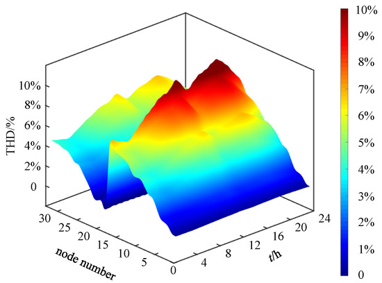
Figure 6.
Harmonic voltage distortion at all buses over 24 h before mitigation.
Figure 5 illustrates that the voltages at individual nodes exhibit temporal fluctuations, with the amplitudes at certain nodes falling below 0.9 p.u. during specific periods, indicating a pronounced undervoltage condition. Along the sequence of node indices, the voltage profile generally demonstrates a declining trend, with the issue being particularly severe at the terminal nodes. Figure 6 presents the distribution of THD% variations across all nodes over a 24 h period prior to mitigation. It is evident that the renewable energy access nodes (12, 18, 25, 29, and 33) and their adjacent nodes experience substantially higher THD levels compared to other nodes, a phenomenon especially prominent during daytime hours (08:00–18:00), when the maximum THD reaches 10%. These results indicate that the inherent volatility and uncertainty of renewable energy output not only elevate harmonic levels at local nodes but also exacerbate the overall harmonic pollution in the system. During periods of high renewable generation, the harmonic injection effect becomes markedly more pronounced, intensifying local power quality issues and underscoring the necessity of deploying compensation devices for effective mitigation.
To enhance power quality in the aforementioned microgrids under high DG penetration, this paper proposes an integrated mitigation strategy founded on coordinated multi-resource optimization. The strategy comprises two components: (i) while maintaining the active-power output of DG inverters, their residual capacity is prioritized for the suppression of harmonic components and the mitigation of voltage deviations; (ii) SAPFs are deployed to further attenuate network harmonics and support voltage regulation, thereby improving overall system power quality. The NNC method, combined with a weighted Euclidean distance approach, is employed to obtain the Pareto-optimal solution set and determine the final optimal configuration scheme; the resulting optimal SAPF locations are identified as nodes 10, 17, 18, 22, and 33. The effectiveness of the proposed strategy is demonstrated in Figure 7 and Figure 8. Figure 7 presents the 24 h nodal voltage profiles, while Figure 8 illustrates the corresponding distributions of voltage total harmonic distortion THD after mitigation. The results show significant improvements in both voltage regulation and harmonic suppression: nodal voltages are maintained within the range of 0.97–1.03 p.u., meeting the 3% deviation limit specified earlier, while nodal THD values remain below 4% throughout the day, fully satisfying the prescribed harmonic distortion threshold.
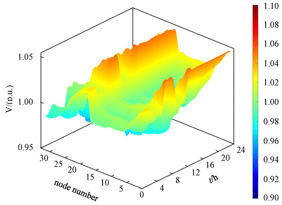
Figure 7.
Voltage distribution of all buses over 24 h after mitigation.
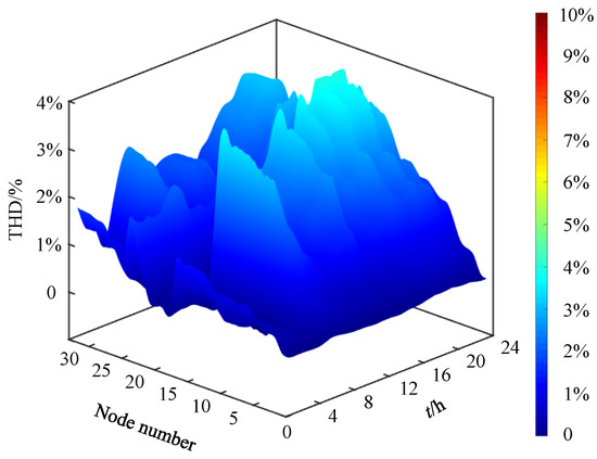
Figure 8.
Harmonic voltage distortion at all buses over 24 h after mitigation.
Figure 9 shows the 24 h harmonic and reactive power compensation outputs of the distributed renewable generation units. While maintaining their active power generation, the DG inverters use their available capacity to mitigate harmonics and voltage deviations in the distribution network. In Figure 9, and represent the 24 h harmonic and reactive compensation capacities of the wind turbine units connected at nodes 12 and 18, respectively, whereas , and correspond to those of the photovoltaic units connected at nodes 25, 29, and 33, respectively. Figure 10 and Figure 11 present the 24 h reactive power and harmonic compensation capacities of the SAPFs, respectively. These results indicate that, by coordinating their available capacity while meeting active power constraints, the DG units play a significant role in suppressing harmonics and supporting voltage regulation, thereby reducing the need for dedicated compensation equipment.
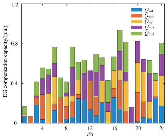
Figure 9.
The 24 h harmonic and reactive power compensation capacity of the DGs.
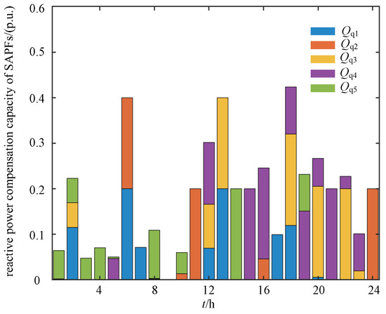
Figure 10.
The 24 h reactive power compensation capacity of the SAPFs.
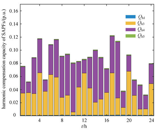
Figure 11.
The 24 h harmonic compensation capacity of the SAPFs.
Table 1 presents the total 24 h harmonic and reactive compensation capacities of each distributed renewable generation unit, along with the corresponding totals for the SAPFs. Based on Equation (1), the power quality mitigation cost for the configuration scheme in Table 1 is calculated to be 2560 CNY.

Table 1.
Optimal Configuration Results for Harmonic and Voltage Deviation Compensation Based on NNC–HEOA Method.
In summary, the coordinated multi-resource optimization strategy proposed in this paper achieves comprehensive mitigation of dispersed voltage deviations and harmonic pollution in the distribution network. The effectiveness of the proposed method is verified through simulation case studies.
4.2. Algorithm Comparison
This section presents a comparative analysis of the HEOA, PSO, GA, and DE algorithms in solving the optimization model developed in this study. To ensure a fair comparison, the population size and the maximum number of iterations of the PSO, GA, and DE algorithms are configured to be identical to those of the HEOA.
In the PSO algorithm, the inertia weight (w), cognitive coefficient (), and social coefficient () are the key parameters controlling the balance between exploration and exploitation [22,23]. The inertia weight w is typically linearly decreased from 0.9 to 0.4 during iterations to enhance convergence stability. Both and are usually set around 1.5 to maintain a good trade-off between local and global search.
In the GA, the crossover probability, mutation probability, and selection strategy [24] are set as follows. The crossover probability () is fixed at 0.8 to ensure effective information exchange between parent chromosomes while maintaining population diversity. The mutation probability () is set to 0.05, introducing sufficient randomness to prevent premature convergence without disrupting the search stability. For the selection operation, the tournament selection method is adopted, as it provides a good balance between selection pressure and maintaining genetic diversity. In addition, elitism is applied to retain the best individual in each generation, enhancing convergence reliability and preventing the loss of high-quality solutions.
In the DE algorithm, two main control parameters are used: the mutation factor (F) and the crossover rate () [25]. In this study, the mutation factor F is set to 0.5, which provides a proper balance between exploration and exploitation by adjusting the differential amplification among individuals. The crossover rate is assigned a value of 0.9, ensuring a high level of information exchange between mutant and target vectors to enhance the global search ability.
To further justify the selection of the HEOA as the core solver for the NNC-based sub-problem, a comparative analysis was conducted with three widely adopted metaheuristic algorithms, PSO, GA, and DE, under identical population and iteration settings. The population size was set to 100 and the maximum number of iterations to 300 to ensure a fair and consistent comparison. As summarized in Table 1 and Table 2, the HEOA achieved the most balanced and cost-effective configuration of DG and SAPF resources, exhibiting lower total SAPF capacity demand and reduced overall mitigation cost compared to the benchmark algorithms. Specifically, the optimization results show that the total economic costs obtained by each algorithm are 2560 CNY for NNC–HEOA, 2612 CNY for NNC–PSO, 2795 CNY for NNC–DE, and 2932 CNY for NNC–GA, indicating a clear superiority of HEOA in achieving more economical resource coordination. This advantage is attributed to the adaptive evolutionary mechanism and self-adaptive exploration–exploitation balance embedded in HEOA, which enhances its convergence efficiency and avoids premature stagnation in local optima.
Table 2.
Comparative Optimization Results of DG and SAPF Configurations for Harmonic and Voltage Deviation Compensation Using Different Algorithms.
The convergence characteristics illustrated in Figure 12 further highlight these advantages. HEOA demonstrates the fastest convergence speed and the lowest final fitness values for both objective functions, (system cost) and (power-quality deviation). In contrast, PSO and DE exhibit slower convergence and higher residual fitness, while the GA produces the least satisfactory results among the compared algorithms. This indicates that the HEOA not only offers better global search capability but also ensures superior robustness and computational efficiency when handling nonlinear, multi-variable, and constraint-coupled optimization problems, such as the coordinated allocation of harmonic and voltage compensation resources in microgrids.
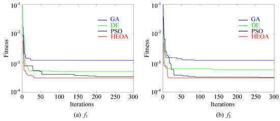
Figure 12.
Fitness curves of and under different optimization algorithms.
5. Conclusions
This paper presents a coordinated optimization framework for harmonic and voltage compensation in microgrids, integrating the operation of DG inverters and dedicated compensation devices. The proposed model simultaneously considers investment, operation, and performance penalties to achieve a balance between economic efficiency and power quality improvement.
(1) The developed unified coordination model effectively describes the coupling and coordinated allocation among the active, reactive, and harmonic compensation capacities within DG inverters, enabling optimal utilization of multiple mitigation resources.
(2) The dual-objective optimization model combines economic and technical objectives under the NNC framework, providing stable and physically feasible optimization results.
(3) Case studies on the IEEE 33-bus system verify that the proposed method can effectively reduce total cost while improving the overall harmonic suppression and voltage regulation performance. Compared with conventional heuristic algorithms such as PSO, the proposed approach exhibits better convergence stability.
Overall, the proposed coordinated optimization strategy achieves a balanced enhancement of both economic efficiency and technical performance, providing a valuable reference for future design and operation of power quality management systems in microgrids.
Author Contributions
Methodology, R.Y. and Y.Z.; Software, T.L.; Formal analysis, Y.L.; Investigation, R.Y. and Y.Z.; Data curation, Y.L.; Writing—original draft, T.L.; Writing—review & editing, H.B. All authors have read and agreed to the published version of the manuscript.
Funding
This research was funded by the Science and Technology Project of China Southern Power Grid Co., Ltd. (No. ZBKJXM20232297).
Data Availability Statement
The original contributions presented in this study are included in the article. Further inquiries can be directed to the corresponding author.
Conflicts of Interest
Authors Yiyong Lei and Yawen Zheng were employed by the China Southern Power Grid Co., Ltd. The remaining authors declare that the research was conducted in the absence of any commercial or financial relationships that could be construed as a potential conflict of interest.
References
- Zhan, Y.; Xie, X.; Zhang, X. Security Region-Based Probabilistic Stability Analysis of Sub/Super-Synchronous Oscillation in Wind Power Integrated Power Systems. IEEE Access 2024, 12, 160776–160783. [Google Scholar] [CrossRef]
- Lin, L.J.; Jia, Q.Q.; Lv, C.H.; Liang, J.F.; Luo, P. Partitional Collaborative Mitigation Strategy of Distribution Network Harmonics Based on Distributed Model Predictive Control. IEEE Trans. Smart Grid 2023, 14, 1998–2009. [Google Scholar] [CrossRef]
- Tian, S.Y.; Jia, Q.Q.; Xue, S.W.; Shi, L.; Lv, C.H.; Bu, L.Y.; Zhou, W. Two-layer model of siting and sizing for active power filters and static var generators considering reactive power capability and active power curtailment of DGs. IET Gener. Transm. Distrib. 2022, 16, 2913–2927. [Google Scholar] [CrossRef]
- Dehaghani, M.N.; Korõtko, T.; Rosin, A. AI Applications for Power Quality Issues in Distribution Systems: A Systematic Review. IEEE Access 2025, 13, 18346–18365. [Google Scholar] [CrossRef]
- Singh, Y.; Singh, B.; Mishra, S. Control of Single-Phase Distributed PV-Battery Microgrid for Smooth Mode Transition with Improved Power Quality. IEEE Trans. Ind. Appl. 2022, 58, 6286–6296. [Google Scholar] [CrossRef]
- Sahli, A.; Krim, F.; Laib, A.; Talbi, B. Model predictive control for single phase active power filter using modified packed U-cell (MPUC5) converter. Electr. Power Syst. Res. 2020, 180, 106139. [Google Scholar] [CrossRef]
- Afonso, J.L.; Tanta, M.; Pinto, J.G.O.; Monteiro, L.F.; Machado, L.; Sousa, T.J.; Monteiro, V. A review on power electronics technologies for power quality improvement. Energies 2021, 14, 8585. [Google Scholar] [CrossRef]
- Khergade, A.V.; Satputaley, R.J.; Borghate, V.B.; Raghava, B. Harmonics Reduction of Adjustable Speed Drive Using Transistor Clamped H-Bridge Inverter Based DVR with Enhanced Capacitor Voltage Balancing. IEEE Trans. Ind. Appl. 2020, 56, 6744–6755. [Google Scholar] [CrossRef]
- Aljumah, A.S.; Alqahtani, M.H.; Ginidi, A.R.; Shaheen, A.M. Improved Artificial Hummingbird Algorithm for Optimal Allocation of SVCs in Distribution Networks to Maximize Energy Efficiency. J. Mod. Power Syst. Clean Energy 2024. early access. [Google Scholar] [CrossRef]
- Djalal, M.R.; Robandi, I.; Prakasa, M.A. Stability enhancement of sulselrabar electricity system using mayfly algorithm based on static var compensator and multi-band power system stabilizer PSS2B. IEEE Access 2023, 11, 57319–57340. [Google Scholar] [CrossRef]
- Li, X.; Wang, H.; Li, J. Power Quality Control and Multi-Objective Optimization Compensation Strategy for Grid-Connected Multi-Functional Inverters. In Proceedings of the 2024 China International Conference on Electricity Distribution(CICED), Hangzhou, China, 12–13 September 2024; pp. 969–974. [Google Scholar] [CrossRef]
- Choi, W.; Lee, W.; Han, D.; Sarlioglu, B. New configuration of multifunctional grid-connected inverter to improve both current-based and voltage-based power quality. IEEE Trans. Ind. Appl. 2018, 54, 6374–6382. [Google Scholar] [CrossRef]
- Maganti, S.; Padhy, N.P. A feedback-based flexible compensation strategy for a weak-grid-tied current-controlled converter under unbalanced and harmonic conditions. IEEE Trans. Ind. Appl. 2022, 58, 7739–7753. [Google Scholar] [CrossRef]
- Zobaa, A.F. Mixed-integer distributed ant colony multi-objective optimization of single-tuned passive harmonic filter parameters. IEEE Access 2019, 7, 44862–44870. [Google Scholar] [CrossRef]
- Cao, W.; Liu, K.; Wu, M.; Xu, S.; Zhao, J. An improved current control strategy based on particle swarm optimization and steady-state error correction for SAPF. IEEE Trans. Ind. Appl. 2019, 55, 4268–4274. [Google Scholar] [CrossRef]
- Yu, L.L.; Zhang, L.H.; Meng, G.J.; Zhang, F.; Liu, W.X. Research on multi-objective reactive power optimization of power grid with high proportion of new energy. IEEE Access 2022, 10, 116443–116452. [Google Scholar] [CrossRef]
- Dai, Z.Q.; Pei, X.; Hu, W.; Wang, H.T.; Xu, Y.N.; Tao, T. Research on Active and Reactive Power Coordinated Dispatching of Distribution Network Considering Reactive Power Optimization Configuration. In Proceedings of the 2025 IEEE 3rd International Conference on Power Science and Technology (ICPST), Kunming, China, 16–18 May 2025; pp. 652–657. [Google Scholar] [CrossRef]
- Wang, J.; Zhou, N.; Ran, Y.C.; Ran, Y.H.; Wang, Q.G. Optimal operation of active distribution network involving the unbalance and harmonic compensation of converter. IEEE Trans. Smart Grid 2019, 10, 5360–5373. [Google Scholar] [CrossRef]
- Lian, J.; Hui, G. Human evolutionary optimization algorithm. Expert Syst. Appl. 2024, 241, 122638. [Google Scholar] [CrossRef]
- Wu, Y.K.; Lee, C.Y.; Liu, L.C.; Tsai, S.H. Study of reconfiguration for the distribution system with distributed generators. IEEE Trans. Power Deliv. 2010, 25, 1678–1685. [Google Scholar] [CrossRef]
- Mazin, H.E.; Nino, E.E.; Xu, W.; Yong, J. A Study on the Harmonic Contributions of Residential Loads. IEEE Trans. Power Deliv. 2011, 26, 1592–1599. [Google Scholar] [CrossRef]
- Jain, M.; Saihjpal, V.; Singh, N.; Singh, S.B. An overview of variants and advancements of PSO algorithm. Appl. Sci. 2022, 12, 8392. [Google Scholar] [CrossRef]
- Iqbal, H.; Sarwat, A. Design and Implementation of Hybrid GA-PSO-Based Harmonic Mitigation Technique for Modified Packed U-Cell Inverters. Energies 2025, 18, 124. [Google Scholar] [CrossRef]
- Shi, X.H.; Liang, Y.C.; Lee, H.P.; Lu, C.; Wang, L.M. An improved GA and a novel PSO-GA-based hybrid algorithm. Inf. Process. Lett. 2005, 93, 255–261. [Google Scholar] [CrossRef]
- Song, Y.; Cai, X.; Zhou, X.; Zhang, B.; Chen, H.; Li, Y.; Deng, W. Dynamic hybrid mechanism-based differential evolution algorithm and its application. Expert Syst. Appl. 2023, 213, 118834. [Google Scholar] [CrossRef]
Disclaimer/Publisher’s Note: The statements, opinions and data contained in all publications are solely those of the individual author(s) and contributor(s) and not of MDPI and/or the editor(s). MDPI and/or the editor(s) disclaim responsibility for any injury to people or property resulting from any ideas, methods, instructions or products referred to in the content. |
© 2025 by the authors. Licensee MDPI, Basel, Switzerland. This article is an open access article distributed under the terms and conditions of the Creative Commons Attribution (CC BY) license (https://creativecommons.org/licenses/by/4.0/).