Abstract
With more hybrid heating systems available, there is a need to optimize energy use intelligently from the end-consumer perspective. This paper focuses on a multi-criteria heating system optimization to optimize cost, carbon emission, and comfort level of building occupants. A discrete Multi-Objective Model Predictive Controller (MO-MPC) algorithm is proposed to optimally utilize two heating sources connected to a building, namely district heating (DH) and a building-integrated electrical heat pump (HP). The model is tested on a real-world building case simulated with a gray box building model. The results are compared to a conventional PID controller as well as the MPC scheme, each with a single heating input, and eight different cases are constructed to make this comparison more visible. The results indicate that, using MO-MPC, a cost saving of up to 10% and emission saving of up to 13% can be reached without additional thermal discomfort, while the potential savings on cost and emission with the hybrid system can be up to 25% and 77%, respectively. Further, a sensitivity analysis on price and emission parameters is conducted to investigate the changes in the provided solution.
1. Introduction
Building heating systems, used in commercial and residential buildings, are crucial and inseparable parts of our societal and individual lives. They provide us with comfortable—or near comfortable—indoor conditions needed to perform daily activities. At the same time, indoor heating and cooling account for more than 50% of energy consumption in Europe [1]. While it specifies a great amount of energy consumption, it also entails that, on a domestic scale, this sector holds a huge opportunity to save energy.
Centralized heating resources are among the most popular means of domestic heating. District heating as a traditional supplier is still well-established as a primary means of heating in urban areas in Europe. However, increasing energy prices over the past few years, lower availability, and environmental concerns surrounding this system threaten the supply of clean and uninterrupted energy in a desired indoor environment for the end-user. Environmentally speaking, in the EU, the second major heat production sources are natural and manufactured gases, accounting for 31.5%, right after renewable energies at 33.5% [2]. This signifies the heavy reliance of the district heating system on highly CO2-emitting and polluting sources. Secondly, the average price of DH in European countries has almost doubled between 2000 and 2015 [3].
A heating supply with a single centralized resource can be inadequate and unreliable. The recent advancement and application of hybrid heating systems, providing flexibility and higher energy efficiency, can be proposed as a solution to these issues. Building-integrated heat pumps (HPs) are one of these systems that have been proven to operate well with the central DH systems. They are rapidly gaining popularity in countries with cold winter climates, such as Germany, Sweden, Denmark, and Austria, due to their decreasing costs and government incentives [4]. The number of buildings supplied by HP has reached 16% of buildings across European countries, with 20 million installed units by 2022 [5]. Not only are they able to assist in supplying the heating demand in cold seasons, but these units also provide a highly efficient source of heating for end-users [5]. This generally results in lower energy bills for building managers and, more importantly, a lower environmental footprint. It is to be noted that in the literature, there are two main categories of hybrid heating systems. In the first type, the HP is working not separately but as a part of a low-temperature DH, otherwise known as 5th-generation DH, which is not the focus of this paper. We assume that HP and DH are working in parallel, and each can individually deliver heat to the consumers.
With hybrid heating systems in place, the control of the system becomes increasingly challenging. Single-resource heating systems are generally controlled by Rule-Based Controllers (RBC)—e.g., on–off controllers—and Proportional–Integral–Derivative (PID) controllers [6], whose main aim is to regulate indoor temperature rather than energy saving. Additionally, the conventional controllers not only have an inherent response delay but also perform poorly under changing systems, which makes them not fully efficient in heating systems with volatile inputs [7]. Furthermore, While these control algorithms are adequate for single heating systems, hybrid systems require a more sophisticated controller to find the optimal heating resources. Model Predictive Controller (MPC) is a superior alternative that offers future control action prediction and fast response and solves an optimization algorithm, all at the cost of being more computationally expensive. In this study, we try to adapt and make a fair comparison of this controller’s performance with the PID algorithm in a hybrid heating context.
1.1. Related Work
The co-existence of building-level HP and DH has been investigated in many studies, especially as a means for energy and cost saving. Reda et al. [8] investigated the hybrid DH and solar-assisted HP hybrid system to provide heat to an office building in Finland. Their results revealed that a 19% renewable heating share in the heating season can be achieved. Hermansen et al. [9] investigate the cost-saving of an MPC-controlled hybrid heating system with both DH and HP, based on time-varying electricity prices. A 23% cost was saved, while authors argue that flexible taxes and fees on the Danish energy market on both DH and electricity prices can make this even more significant and encourage customers to take more energy-efficient decisions. A hybrid solar-assisted DH with local HP and auxiliary gas heater is modeled by Abokersh et al. [10] in TRNSYS 18, a transient system simulation software. Thermal energy efficiency and economic cost of the system are assessed in two different RBC strategies. In another research by Liu et al. [11], a DH coupled with geothermal HP is considered with different heat control loops in place. The capacity and investment cost were considered in this study, and the hybrid system’s viability and competitiveness are compared with a normal DH. Liu et al. [12] studied a solar-assisted HP and DH hybrid heating system to lower operating cost and maximize renewable energy use. TRNSYS 18 is used to model the heating system with an RBC for the solar and heat loop. They have reached economic savings of at least 72% in the latter by leveraging solar energy. A DH, borehole thermal energy storage, and HP were studied by Fiorentini et al. [13] to investigate the effect of the hybrid system on the cost and carbon emission of the system. The most savings they can achieve compared to a storage-less system are nearly 10% and 44% for the emission and cost. A ground-source HP and DH is optimized in several cases by Xue et al. [14], prioritizing cost or maximum demand reduction in resources. Their analysis gave a 2.2% reduction in cost in a hybrid solution while increasing the CO2 emissions slightly due to the higher DH emission levels. A comparison of the reviewed literature and the current study is summarized in Table 1.

Table 1.
Summary of the recent related literature and their major focuses compared with the current study.
The control algorithm is the core of hybrid heating systems. MPCs, as a means of thermal system control, have been widely researched. Knudsen et al. [15], a bi-objective MPC algorithm, is used to control the energy consumption considering the cost and CO2 emission of the system on a Danish electrical-based heating system. The findings show that, by leveraging demand response, a significant cost saving can be made compared to a PID-controlled system. In another study by Tarragona et al. [16], an MPC-controlled building connected to an HP, solar panels, and a storage tank was tested under several simulation scenarios. It was concluded that the hybrid system with the controller has significant economic savings compared to the rule-based controller. Baeten et al. [17] investigated using a multi-objective MPC to optimize comfort, cost, and carbon emission separately. They targeted an electrical-based HP and natural gas boiler, aiming to optimize the building’s energy scheme by adopting a demand response program. Finck et al. [18] proposed an economic MPC on an HP and thermal storage heating system in one house. A rule-based controller, as a base case, and two different MPC pricing scenarios are considered to show the demand flexibility capturing of the latter cases and optimize the energy consumption and the total consumer heating cost. Aruta et al. [19] proposed a bi-objective MPC penalizing energy cost and thermal discomfort (using aggregated deviation temperature as the index). A genetic algorithm is used to find the optimal solutions, and the model is tested on a nearly zero experimental building. Apart from the MPC, the fuzzy-logic algorithm has been considered for achieving similar goals. Qi et al. [20] used this concept to control a ground-source HP aiming to save energy and improve thermal comfort. The results show a significant improvement compared to a PID controller. In another study by Underwood et al. [21], the fuzzy-logic controller was used for the same purpose and optimal setpoint tracking.
Gray-box modeling has been used extensively to model building thermal characteristics for MPC applications. In terms of the order of the model (which is specified by the number of capacitors in the model), many studies exist to find the right order. The authors in [22] investigated the Resistor–Capacitor (RC) models used for small and large applications. The review identifies that the commonly used models for building energy simulation are the ISO 13790 (5R1C) [23] and VDI 6007 (7R2C) [24] suggested building models. Another study by Vivian et al. [25] made a comparison between the two mentioned models and realized that the second-order one (7R2C) substantially lowers the Root Mean Square Error (RMSE) by up to 53%, capturing the dynamics of the building more accurately, both for cooling and heating seasons. A study by Yu et al. [26] concluded that the second-order models perform more robustly, while the third-order models are prone to overfitting. The models were tested on a real-world, experimental building [27]. Klanatsky et al. [28] focused on the methods of parameter estimation on a test case and provided a comparison with RC models of different orders, concluding that the third-order model is the most suitable building model to feed predictive controllers. Other studies [29,30] observed that, for both heating and cooling applications in longer periods, first-order models are more accurate than the second-order ones. The complexity of the RC models is quite flexible, and based on the application, higher-order models can be used for specific cases. However, most reviewed research realized that 2nd-order and 3rd-order RC models are adequate for the MPC application of small-scale buildings in heating seasons. Another important aspect of gray-box models is the number of states. Bacher et al. [31] investigated RC models with several states and realized that the two-state and three-state models (where usually one state represents the measurable indoor air temperature and the remaining states correspond to latent, unmeasured thermal dynamics) are performing the best in terms of model robustness—using statistical metrics such as the auto-correlation function and residuals—for simulating a single-zone building heating system.
1.2. Research Aims and Contributions
In the existing literature, the MPC is used extensively in building energy control. However, there is a gap in using the controller to incorporate more optimization criteria. Addressing hybrid energy systems from a consumer perspective is another shortcoming observed in the literature. The result of this study will help building simulators, energy providers, and most importantly, building managers in operating buildings to make a more optimal decision locally while reflecting the energy supply chain constraints and advantages. The main contributions of this paper are as follows:
- A multi-objective predictive controller designed to consider cost, emissions, and comfort level of the building’s indoor environment. The hybrid heating system is supplied by a heat pump and district heating.
- Proposing an MPC and a system architecture to assist the process of applying it to real-world hybrid-heated buildings
- Competitiveness analysis of district heating versus heat pumps in the Swedish energy market using real-world data.
- In a sensitivity analysis, investigating the control behavior under different cost, emission and outdoor weather condition scenarios.
The rest of the paper is organized as follows: Section 2 provides a detailed framework and system architecture of the hybrid heating system considered in this study. It further explains the minimum necessary data for the controller to operate and how they can be obtained. Section 3 shows the simulation results under different generated case studies and compares them against one another. Section 4 discusses the results and authors’ findings based on the findings in this paper. Section 5 provides a summary and possible future study paths based on our research. Finally, Appendix A describes detailed building simulation parameters that are used in this study.
2. Materials and Methods
2.1. System Overview—Hybrid Heating System
The system under study is a hybrid heating system, including centralized DH and a building-integrated HP, connected to a single-family building with a single heating zone. The overall system framework is depicted in Figure 1. Each system has separate heat delivery pipes, meaning that they work independently. The HP considered in the study is an air-to-water system based on a commercial model in [32], and it is powered by electricity. It was assumed that the maximum building heat demand in the simulated week is smaller than each heat supplier’s capacity, meaning that one heating unit can supply the entire demand at any time.
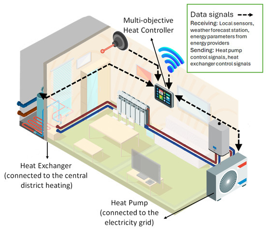
Figure 1.
General framework of the studied system.
The energy parameter signals, namely emission and cost, are received from energy providers. The DH delivers heating with pipelines and a heat exchanger unit connected to the building. Based on the study location, it is assumed that the DH prices are fixed throughout the year, while the emission level is changing with one-hour resolution. As for the electricity, both prices and emission levels follow hourly time-series data. More details on the energy prices are explained in Section 3.1.
2.2. System Architecture: Cloud and Local Data
In the application of the control system described here, it is assumed that the controller has access to several data sources. These data are received either locally through the sensors installed in the case study or through communication with data providers. We have identified several signals that are transmitted from the energy providers and weather stations, which are (1) The day-ahead dynamic prices/emissions from the electricity provider; (2) the day-ahead heating prices/emissions from the DH provider (considered as fixed-price contracts over a year); and (3) the day-ahead ambient temperature/solar irradiance forecast.
The rest of the data is measured locally in the case study, which includes (1) the flow of the air handling unit (AHU) or exhaust air flow and its temperature to calculate the ventilation losses; (2) the estimated process energy, based on occupancy and indoor activity, to calculate the process energy input; and (3) the indoor temperature recordings to fine-tune the model predictions according to the subject building.
2.3. State-Space Building Model
At the core of the MPC algorithm is the system modeling, which arguably determines the overall accuracy and efficiency of the controller. A state-space model of the building is adopted to represent the building’s thermal characteristics in this study. This study uses a discrete linear state-space model formulated as a Stochastic Differential Equation (SDE), shown in (1), as part of the controller. It is to be noted that the continuous state-space model of the building is discretized using the exponential discretization method.
where k is the discrete time-step index, X is the state vector of the building, U is the system input vector (measured disturbances), is a vector with the system noises (unmeasured disturbances), and Y is a scalar with the output (indoor temperature prediction).
The mentioned state-space model is based on a physical gray-box modeling of the building, approximated by RC electrical networks. A more in-depth description of the 3R2C model can be found in Appendix A. The model and the estimated parameters were obtained from [26], which can be referred to for the exact estimated parameters.
2.4. Multi-Objective Model Predictive Controller (MO-MPC)
One of the benefits of the MPC is the capability to solve an optimization problem. Here, a discrete, non-linear MO-MPC is chosen as the core controller. The goal of the problem is to incorporate three elements to find the optimal solution, which includes the total operating cost of the heating system, the carbon emission of the heating system, and the comfort deviation of the occupants.
A multi-objective formulation is developed to tackle this, and a weighted-sum method is used to solve the problem shown in Equation (2). Equations (3)–(5) indicate each mentioned objective expression. It is worth noting that in (5), the operative temperature of the heating zone is chosen to represent the thermal comfort. More detailed information on this comfort index is explained in Appendix B. In Equation (6), the Coefficient of Performance (COP) of the HP is calculated based on outdoor temperature according to the manufacturer’s datasheet [32]. Equation (7) is the relation between HP electrical power and heating power. Finally, Equations (8)–(10) are the DH power limits, HP electrical power limits, and indoor temperature bounds, respectively.
Normalization techniques are usually used in these problems with different objective ranges to ensure an equal effect on the decision variables. Here, a common approach in MPC, namely the min–max normalization, is utilized. Each objective is normalized using min–max normalization, as in , to fall between (0, 1). The minimum and maximum values are determined by a series of pre-simulations on one objective at a time. By running the simulation single-objectively, we found the minimum and maximum of each objective as follows:
- The cost objective has a value between 251 and 368.
- The emission objective has a value between 2.0 and 17.2.
- The discomfort index objective has a value between 1 and 192.
The above information was used as the mix–max normalization bounds to normalize the objectives as explained above.
subject to: Equation (1),
where , , and are the cost index in (SEK), carbon emission index in (kg CO2) and discomfort index in (°Ch), and the specifies the normalized values; is the number of time steps in the simulation horizon; and are the electricity and DH time-series energy prices in (SEK/kWh); and are the electricity and district heating network time-series CO2 emission levels in (kg CO2/kWh); and are the COP of HP and the DH efficiency; and are the outdoor (ambient) and the operative temperature in (°C); , , and are the efficient heating power delivered by DH and HP and the electrical power of HP (in kW); and and are the lower and upper temperature setpoints; is the thermal comfort temperature set.
It is worth noting that —standing between and —is considered as the ideal temperature for the occupants and is focused on in (5) as a soft constraint. Additionally, broader hard constraint bounds are applied to make sure the temperature does not protrude beyond certain levels. Generally, thermal comfort is a broad topic measured by many indoor air quality indices. Here, the operative temperature is chosen to represent this (refer to Appendix B). , , and in (2) are the weighted sum average coefficients and are determined as follows. The problem is solved iteratively with different weights. In all solutions, the sum of the three equals to 1, and the interval of change is 0.1. For instance, in one scenario with weights equal to , , and , the simulation is focused on total cost minimization, and the other two objectives are not considered. The algorithm of the adopted controller is shown in Algorithm 1. In this algorithm, k and l are discrete time steps and control horizon indices. is the initial state equal to .
| Algorithm 1 Multi-Objective Model Predictive Controller |
|
The simulation was conducted on an online notebook in the Google Colaboratory environment [33], using the Python programming language version 3.11 [34]. The Casadi library package is used to model the controller and the optimization problem with the in-built non-linear IPOPT solver [35].
3. Results
This section highlights the results of the simulation-based study in this work. It is worth noting that several assumptions are made in our work, which are as follows:
- The changes in building insulation wear and tear and efficiency of the heating systems are negligible during the simulation period.
- The size of the heating systems is selected in the sense that each heating resource can independently supply the building’s heating demand.
- The heating demand consists only of the space heating, and the domestic hot water demand is not considered.
3.1. Case Study
The simulation result of the proposed controller is compared against PID controllers. To do so, several cases are constructed to make the comparison more tangible. These cases are defined based on the used heating resource and the objective of the simulation and are shown in Table 2. Cases A and B represent PID-controlled heating systems with a single input—HP in Case A and DH in Case B—and serve as the baselines. Cases C and D are MPC-controlled single-input (either HP or DH) with all three objectives and equal weights. Cases E, F, and G are single-objective MPCs with hybrid input (both HP and DH), with the objective focusing on cost, carbon emission, or comfort level one at a time. Finally, case H is one optimal multi-objective hybrid input case with equal weights (, , ).
Table 2.
Simulation cases based on the model, objective(s), and input source(s).
The simulation is conducted over a week in the cold season, the first week of December 2023, with the weather conditions [36] and local energy prices of Malmö, Sweden, in the mentioned period. Figure 2 illustrates weather data and energy-related input signals (also known as measured disturbances in the control context). The dynamic spot market electricity prices [37] and the fixed DH prices for small buildings [38] located in southern Sweden are obtained from open data sources. As the paid electricity bill for the private customer includes certificates and additional network charges, a 66% electricity cost is added to the hourly spot market costs. The electricity emission data [39] are available online, and the DH emission factor according to the Swedish National Board of Housing (Boverket) equals 56 g CO2/kWh [40]. Since this study focuses on creating added value on the changing energy parameters, a dynamic DH emission is required. Therefore, a Gaussian random hourly emission scenario with the mean equal to 56 g CO2/kWh and sigma equal to 7.5 g CO2/kWh is generated, with the assumption that the emission levels are the highest in the daily coldest hours and peak usage of DH, and is illustrated in Figure 2. This assumption is grounded on the fact that in early morning hours and late afternoon, due to colder outdoor temperatures and typical social patterns, energy demand for space heating and hot water surges. Consequently, more air-polluting and lower-priority centralized heating sources are used, resulting in higher carbon emissions of the DH system [41].
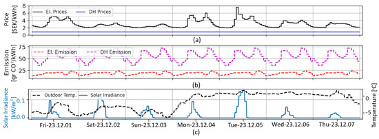
Figure 2.
Input signals (also known as measured disturbances) including (a) electricity and district heating hourly prices, (b) electricity and district heating hourly emissions, and (c) hourly outdoor temperature and global horizontal solar irradiance.
The building, heating system, and controller are also other components that require modeling data for simulation. The building data is obtained from the ZEB living lab project, an experimental building developed for thermal analysis of buildings and their energy resources. The gray-box modeling of this building and estimated thermal parameters are presented in Appendix A. The heating system parameters considered in this study are shown in Table 3. Additionally, the MPC setpoints, determined based on the data availability and project needs, and PID set parameters, based on the guidelines in [42], are shown in Table 4. It is worth mentioning that the PID set point is considered with a dead band between 21 and 23 °C so that it is comparable with the MPC comfort zone, which has the same thresholds.
Table 3.
Heating systems specification.
Table 4.
Controller setpoints and parameters for the model predictive and the PID controller.
3.2. Simulation Results
The simulation results of the eight constructed cases are presented in Table 5, and the scaled values of each objective for these cases are illustrated and compared in Figure 3. The heat output and operative temperature profile of each case are illustrated in Figure 4. Table 5 shows the objective values for each considered case. Cases A–D all have a single heating input. Cases A and B focus on keeping the temperature at a certain level, while C and D consider all three objectives simultaneously. The data shows that the HP-based PID controller has the highest cost, while the DH-based PID controller case has the highest emission level (almost eight times the former), with both having quite low discomfort. Cases C and D decrease the cost and emission slightly, compared to A and B, compromising the comfort level slightly more. This fact is also reflected in Figure 4a–d.
Table 5.
Numerical results for the studied cases with model predictive controllers and PID controllers in one week of simulation.
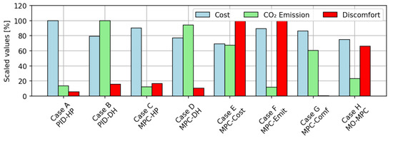
Figure 3.
Scaled cost, carbon emission, and discomfort index of the studied cases using the max-scaling method.
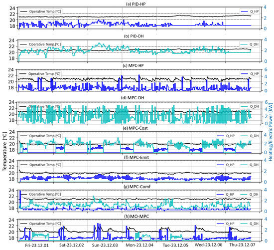
Figure 4.
One-week simulation result, the heating, and the operative temperature profiles for the considered cases.
The rest of the cases are considered to focus on one or a mixture of objective statements (as mentioned in Equation (2)), with hybrid input, trying to minimize their value in cases E-H. Case E demonstrates the least cost while having the highest emission, after Cases B and D. Additionally, Cases E and F each have the lowest comfort. Compared to E and F, Case G has the smallest discomfort level while having relatively high cost and emission objectives. Finally, the results of case H stand between the extreme cases, considering all criteria at once, as discussed before, with equal penalty weights.
The data in the table reveals that, in terms of cost, the base case (case A) is the most expensive operation of the system, while case E has the lowest expense, followed by cases H, D, and B. In terms of emissions, case F has the lowest carbon footprint, followed closely by the base case. Finally, comparing the comfort level of the generated cases indicates that case G has the lowest discomfort, while cases E and F have the highest. Finally, case H considers the three objectives simultaneously, and it is observed that the objective values are positioned between the single-objective cases. With 9% more cost compared to case E, case H has half the emission of this case with a higher comfort level. Additionally, the results shown in Figure 3 indicate that in the last-mentioned case (Case H), approximately a 25% saving on cost and 75% saving on carbon emission can be achieved compared to the extreme cases while lowering the comfort slightly (equal to 65% of the least comfortable case).
After conducting the above simulation, to obtain a better perspective of the influence of each objective and multiple criteria-based solutions, we focused on a multi-objective simulation. The problem was initially solved using two objectives at a time by setting the weight of the third objective to zero. The weights of the remaining two objectives were varied in 0.1 increments from 0 to 1, ensuring they always summed to 1. The results for three different combinations of bi-objective problems are calculated and illustrated in Figure 5. Some specific weighted scenarios are highlighted, and further, the results are compared to PID controller cases in these figures.
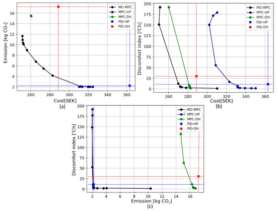
Figure 5.
The Pareto Frontier of MO-MPC bi-objective problem solution with different combinations of weights from 0.1 to 1 for (a) cost versus carbon emission minimization with , (b) cost versus discomfort minimization with , and (c) carbon emission versus discomfort with . The results are compared with the PID controller values(the dashed line are guide lines to specify the PID case positions in the figure.
Finally, the problem was solved with all three objectives explained previously in Section 2, and the results are shown in a 3D plot in Figure 6. The figure is generated as a dotted line and a surface and compared to the values of PID controllers in cases A and B. In the right figure, the color map is the discomfort index, coloring the z-axis. In the left figure, the red triangle is a reference plane.
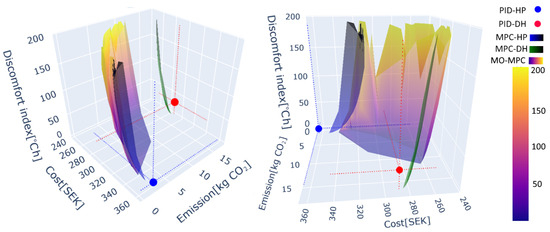
Figure 6.
The Pareto Frontier of MO-MPC and single-input MPC (MPC-HP and MPC-DH cases) of the system with three objectives, namely cost, carbon emission, and discomfort index, in 3D plots (from two perspectives of the same plot).
3.3. Sensitivity Analysis
In this subsection, we present the change in the output objectives, namely cost, emission, and discomfort index, and the use of energy resources and their dependency on the input signals and external conditions.
3.3.1. Price Changes
One of the simulation’s uncertainties is the dynamic electricity prices in Sweden. These prices are often volatile and dependent on network constraints, demand, renewable energy production, and weather forecasts. It is to be noted that, at the time of writing this article, the DH prices are fixed for one year and do not change until the year after, in the Swedish context [38]. Here, we conducted the sensitivity analysis by fixing the DH prices and changing the electricity prices. Scenarios are constructed by changing the electricity price signal proportionally from −50% to +50%. It is worth noting that the results can be perceived as the changes representing the ratio between two price signals. For example, a +20% electricity prices () scenario is the same as a 1.2 ratio between electricity and DH prices (). The results are shown in Figure 7a–c. Figure 7b,c represent the share of HP and DH in each case. It is worth noting that Cases A–D with the PID controller and single-input MPC do not display changes in their energy use and therefore are not considered in price and emission changes in this and the following subsection.
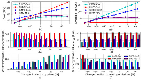
Figure 7.
Sensitivity analysis: (a–c) showing the system cost changes and heating resources’ share when electricity prices change, while (d–f) show the emission changes and heating resources’ shares when the emission level of district heating changes.
The results in this illustration indicate that, in case D, a 20% increase in electricity prices results in a sharp decrease of 82% in HP, meaning that it drives the algorithm to virtually always prioritize DH over HP. The price reduction of over 40%, on the other hand, results in shifting to HP for most of the time, and cheaper electricity prices will make DH almost impractical to use at all times. In case H, however, the shift in energy sources is more moderate. A 40% electricity price decrease has more effects on this case, presumably because the HP has lower emissions; this case prioritizes HP even more than case E.
3.3.2. Emission Changes
Another case-sensitive parameter is the level of network emissions. Hourly emission data, reflecting the resource mix of the DH and electricity, were more difficult to access at the time of publishing this paper. The electricity emission, while it might differ to some extent, is generally quite low in Sweden and considered unchanged. The DH emission, however, can vary substantially based on the season or the sources of heating that are used. To consider these changes, scenarios changing the emission from −90% to +40% are considered. It is worth noting that according to [40], the DH emission level can be more volatile, and therefore higher changes compared to the previous analysis on electricity have been considered. The results, such as the changes in the emission and the share of heating systems, are shown in The results are shown in Figure 7d–f.
The results show that the emissions in cases E and G are quite proportional to the increased emission factor of DH, and the share of HP and DH stays unchanged (the cyan and blue bars in Figure 7e,f. This reflects the fact that emission is not considered in their objective function. In cases F and H, however, the controller behaves differently. In case F, it changes the energy use only for scenarios where emission is lowered more than 80% (the red bars in Figure 7e,f). This is due to the fact that the HP emissions are drastically lower than the DH’s. In case H, the changes in energy mix happen across all emission scenarios. In other words, the DH is gradually being used more, lowering the emission levels. This reflects the fact that the three objective values should be equal in all scenarios in this case.
3.3.3. Weather Changes
The alterations in weather conditions—especially outdoor temperature—can affect the results in two ways. Firstly, since the efficiency of the HP is weather-dependent (see Equation (6)), the HP is less efficient at lower temperatures. Secondly, the heating load of the entire system will increase when the temperature drops. Consequently, a sensitivity analysis is conducted to demonstrate the heating system’s behavior in response to changes in temperature.
To evaluate the controller’s performance under different weather conditions, six temperature scenarios were created, varying the outdoor temperature in 5 °C increments from −15 °C to +10 °C relative to the base case. In the base case, the outdoor temperature ranges between −5 °C and 0 °C; therefore, the coldest scenario corresponds to temperatures between −20 °C and −15 °C, while the warmest scenario represents conditions between +5 °C and +10 °C. The reason for this range is that the assumed HP’s minimum operating temperature stands at −20 °C, and the heating system is usually utilized not above +10 °C ambient temperature. The value of each objective and the share of DH and HP in each case over the simulation horizon are depicted in Figure 8 and Figure 9, respectively. In the latter figure, the bars corresponding to DH and HP are marked.
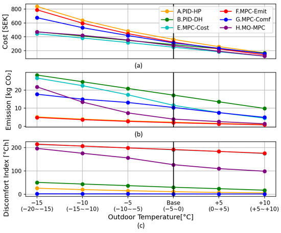
Figure 8.
Sensitivity analysis on the outdoor temperature showing the value of (a) cost, (b) emission, and (c) discomfort index for the simulation cases when the outdoor temperature varies.
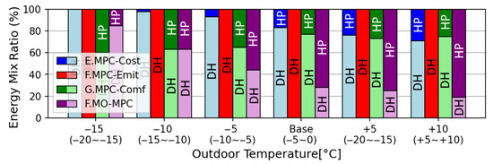
Figure 9.
Sensitivity analysis on the outdoor temperature showing the share of HP and DH in percentage for the simulation cases when the outdoor temperature varies.
The results in Figure 8 show that with the drop in temperature, all objective criteria increase. In terms of cost, the increase is more moderate in cases E and H, which prioritize cost and mix of objectives. The emission increases steadily for all scenarios, with case F being less pronounced. In terms of comfort, cases A, B, and G have retained almost the same level of comfort with the changes in temperature. It is worth noting that in this graph, cases C and D, which involve only a single input, are excluded to avoid overcrowding the figure.
The share of energy resources shown in Figure 9 demonstrates that at lower temperatures, cases E and H experience more DH use, where at a −15 temperature drop, almost all load is supplied by the DH. The reason, as mentioned earlier, is the lower COP of HP in colder climates. Case F supplies the entire demand with HP regardless of the temperature since the emission level of HP is still much lower than that of DH. The only scenario where HP use stays unchanged and even increases slightly with the drop in temperature is case G. In this comfort-based case, the cost and emission factors are excluded, which makes the input sources unimportant to the algorithm, as long as the discomfort is minimized. The slight increase in HP use could be the effect of its higher efficiency in general. It is worth noting that cases A, B, C, and D are excluded since they are single-input cases, wherein cases A and C, HP share is always 100%, and in cases B and D, DH share is always 100%.
4. Discussion
The prioritization of objectives is a key consideration in addressing multi-objective problems. The results in Table 5 suggest that the three objective goals are virtually in “contrast”, a term proposed by Sameti and Haghighat [43]. This means that an increase in one will lead to a decline in the other. In other words, opting for cost minimization will increase the emissions and discomfort, while opting for carbon minimization will increase the cost and thermal discomfort, and so on. Here, case H is merely an example of a candidate Pareto frontier, which considers equal weights and importance for all three objectives. Overall, a strategy must be taken by the stakeholder (building manager, network operator, or both) to determine the weights and make a compromise with the less important objectives. In the literature, there are several articles addressing the weight assignment in such problems. In [6], a standard weighting method is described in which objectives are given equal weights, yielding the initial results. After that, start changing the weights in a way that the sum will still add up to 1 until it has the expected prioritization. Another research [44] has used a lexicographic formulation in an attempt to rank the objectives based on importance. Afterwards, solving the problem with one objective at a time and adding the results as constraints, trying to solve the problem with the next objective. This method is specifically useful when there are many objectives involved in a multi-objective problem.
From another perspective, the significance of input parameters on the results is monitored during the simulation. Parameters such as the efficiency of each heating system, the difference between the cost and emission signals, and the weights definition are the main link between the results and inputs. The ratio between the efficiencies () determines at what ratio between input signals the heating sources are switched on. For instance, if this ratio equals three, it means in cost-based cases the HP is activated when the electricity cost is less than three times the DH cost. This argument is valid for emission levels and the emission signal as well. On top of that, the weighting factors decide which heating source to switch on based on a certain input signal. For example, a higher cost objective weight will prioritize the electricity and DH costs over their emission level.
In terms of the numerical results and the optimal strategy, the proposed MO-MPC outperforms the PID controllers and single-input MPCs. These solutions are compared to MPC cases in 2D and 3D Pareto figures in Figure 5 and Figure 6. Ideally, the solution on the depicted line is optimal, and the ones in the dominated region (above and to the right of the Pareto frontier line) are suboptimal, since at least one Pareto-optimal solution exists that improves one or more objectives without worsening the others. The PID solutions fall into the dominated region, which suggests that they are suboptimal solutions. The single-input MPCs are almost aligned with the MO-MPC curve, which shows they are superior solutions compared to the PID ones. This shows that the algorithm successfully optimizes the hybrid heating system, taking advantage of the price and emission levels during the simulation period.
In terms of the thermal comfort in simulation results, in PID-controlled systems (cases A and B), which prioritize the operative temperature, it has led to a fairly comfortable environment. The discomfort index, however, increases drastically in MPC cases E and F and to some extent in case H. While high discomfort is observed in some MPC cases, the MO-MPC provides this advantage to set how much importance should be given to the discomfort index, since other criteria can play a role. For instance, in case H, the discomfort has increased less intensely while lowering the cost and emission of the system at the same time.
Another remark is that while the proposed controller is functional in other hybrid systems in different contexts, the share of the heating resources might vary. This depends on the input energy parameters, namely the price and emission levels in the target geographical location. The MO-MPC algorithm is otherwise guaranteed to make optimal heating decisions based on the system inputs.
The solution requires both energy systems to be in standby mode and the prices to be meticulously chosen by the operators. In many buildings with hybrid heating sources, HP is merely a backup resource for when the demand is high or sometimes manually switched on by the building manager based on individual preferences. Additionally, for such a system to exist and make decisions automatically, energy prices ought to be determined more competitively by the energy provider, taking network and environmental constraints in energy use into account.
Another point of discussion is how to determine the “right” weights (in this context, , , and ). Something that has not been fully addressed in the previous multi-objective research is the authority to tamper with the weights of the proposed solution from different stakeholder perspectives. Based on the theory of Pareto Optimality, the multi-objective solutions in the discussed cases (cases E–H) are at the front of all “Pareto Optimal” solutions with different objective prioritization [45]. However, the “right” weights are often subjectively different—if not in conflict—from a consumer perspective versus a network operator perspective. For instance, the consumer might opt for a maximum comfort level, which, according to our simulation results, has a high cost and emission level. This might be entirely different from the network operation goals. This will raise the question of the level of authority in determining the weights from a consumer perspective. More research is required on how and to what extent each stakeholder can determine the optimization weights.
A further aspect to consider is the scalability of the proposed approach. In this study, we focused on a single-family, single-zone building; however, two distinct scenarios arise when extending the framework to multi-zone buildings. In the first scenario, where each household is equipped with its own heat pump (HP), the algorithm remains scalable, as each apartment can independently benefit from an MO-MPC system. In the second scenario, involving shared heating resources—specifically a common HP—a distributed or centralized MPC architecture would be required. Although several studies have explored such control strategies, the scalability of the present model for these types of buildings still requires validation in further studies.
The results illustrate the prioritization of chosen energies in the Swedish energy market. While the method is general and applicable in any setting and climate, the share of each energy resource is dependent on the input signals (cost and emission) of that market. The relation between these energies can be further assessed in other heat-requiring countries. The heating demand consists of space heating only in this paper. The domestic hot water is another major heat demand. It usually requires a prediction model based on consumers’ living patterns and regulating the hot storage tank temperature/flow accordingly [46,47]. This was out of the scope of this paper but should be highlighted as a future direction in a mixed-method study.
We have identified some limitations in this study. The sum of operative temperature deviations as a thermal discomfort index cannot fully reflect this criterion. It indeed penalizes the higher deviations (especially above one °C) exponentially. This will force the optimization to keep the deviations within one °C. However, this method assumes symmetric discomfort (e.g., 2 °C hotter is considered as uncomfortable as 2 °C too cold), while this does not reflect reality, as some individuals may tolerate higher temperatures more easily than colder. Another limitation is that the comfort level criteria do not account for humidity, air movement, or clothing level, which are part of more advanced thermal comfort models, such as predicted mean vote.
Finally, in this study, both the air-to-water HP and the DH system were modeled with sufficient capacity to individually meet the entire heating demand. This assumption was made to focus on the operational performance of the MPC algorithm, allowing it to determine the optimal allocation between the two heat sources without constraints from component sizing. In practice, the HP would typically operate up to a defined bivalence point, and the DH would supply the remaining load. The MPC framework can easily be extended to include such a capacity limitation, which will be addressed in future research.
5. Conclusions and Future Directions
This paper investigates a hybrid heating system control and provides a practical framework to apply in real-world scenarios. The performance of a Multi-Objective Model Predictive Controller (MO-MPC) that applies different combinations of cost, emission, and comfort level of a hybrid heating system in an individual building. The heating system is composed of a central district heating (DH) with a controllable heat exchanger and a building-integrated heat pump (HP). The results are compared to a conventional PID controller with a single heating resource. The simulation is conducted using electricity and DH market data for a week in the cold season in the Swedish energy market.
Eight cases with different inputs and goals are constructed to compare the systems against one another. The results demonstrate that the MO-MPC algorithm outperforms the PID controller from several viewpoints. The cost saving and emission saving of the MO-MPC can be as high as 10% and 13% compared to the single-input PID system, while the achievable savings on cost and emission with the hybrid system advantage are up to 25% and 77%, respectively. Further, sensitivity analysis shows that changes in electricity prices can heavily affect the optimal solution. Only a 20% increase in electricity prices makes DH virtually always superior to HP in a cost-based solution. This emphasizes the importance of dynamic cost determination by energy providers to have a hybrid solution.
For further development of this research, several elements should be considered or improved to make the system more robust and closer to reality. Here, thermal comfort is measured by the operative temperature. More indices (qualitative and quantitative) will improve the accuracy and validity of this heating system objective. Additionally, the multi-objective weights considered here are essentially examples of the final solution. As discussed in the discussion section, very few studies have investigated consumer choices and heating priorities and how they might affect the energy network. The consideration of domestic hot water prediction was not in the scope of this paper; however, it can add value in terms of making the model more realistic through a mixed-method approach.
Author Contributions
Conceptualization, A.S., P.D., R.M. and R.S.; methodology, A.S.; software, A.S.; validation, A.S.; formal analysis, A.S.; data curation, A.S.; writing—original draft preparation, A.S.; writing—review and editing, A.S., P.D., R.M. and R.S.; visualization, A.S.; supervision, P.D., R.M. and R.S.; project administration, R.M.; funding acquisition, P.D. and R.M. All authors have read and agreed to the published version of the manuscript.
Funding
This research is partially supported by the Knowledge Foundation (Stiftelsen för kunskaps- och kompetensutveckling) for the project titled “Intelligent and Trustworthy IoT Systems” under Grant No. 20220087-H-01.
Data Availability Statement
The original contributions presented in this study are included in the article. Further inquiries can be directed to the corresponding author(s).
Conflicts of Interest
The authors declare no conflicts of interest.
Abbreviations
The following abbreviations are used in this manuscript:
| DH | District Heating |
| HP | Heat Pump |
| MPC | Model Predictive Controller |
| MO-MPC | Multi-Objective Model Predictive Controller |
| PID | Proportional–Integral–Derivative |
| RBC | Rule-Based Controller |
| RC | Resistor–Capacitor |
| AHU | Air Handling Unit |
| COP | Coefficient of Performance |
| I.I.D. | Independent and Identically Distributed |
Appendix A. Gray-Box Model of the Building
In this section, the building simulation model is described. To capture the thermal characteristics of the case study—the “ZEB Living Lab” experimental building [48]—a gray-box model is used. Yu et al. in [26] experimented with different RC networks applied to the same case study with different orders and numbers of parameters and realized that the stochastic 3R2C model, depicted in Figure A1, exhibited the least residual error and performed more robustly on the validation dataset. The same model and parameters are used in this study, which are listed in Table A1.

Figure A1.
Gray-box model representation of the building.
Figure A1.
Gray-box model representation of the building.

Equations (A1)–(A5) describe the details of the building state-space model previously mentioned in Equation (1) in this study. Model states, inputs, and disturbances are shown in (A1). The model parameter matrices are detailed in (A2). Equations (A3) and (A4) are the SDEs of the building. Finally, Equation (A5) is the heat loss through ventilation (or gained through an air handling unit).
where , , and are the indoor, envelope, and outdoor (ambient) temperatures, respectively; and are the indoor and envelope temperature disturbances; , , and are the heat resistance between indoor and envelope, envelope and outdoor, and indoor and outdoor through windows and doors, respectively; and are the heat capacity of indoor thermal mass and the heat capacity of the external walls; is the heat lost (or gained) through ventilation (or air handling unit); is the indoor activity and process energy; and are the active area times the heat gain through windows and through walls based on each surface area; and are the air mass and the air heat unit; and, finally, and are the supplying and exhausting air temperatures of the system.
It is worth noting that the and are considered constant and neutralize one another; therefore, they are not used in this study. and are generated based on the residuals of the RC model. The one-step predictions (residuals) are estimates of the system noise (i.e., the realized values of the incremental Wiener process) added together with the observation noise. They are assumed to be white noise, i.e., Independent and Identically Distributed (I.I.D.).
Table A1.
Gray-box model thermal parameters used in this study.
Table A1.
Gray-box model thermal parameters used in this study.
| Model Name | [°C/kWh] | [°C/kWh] | [°C/kWh] | [kWh/°C] | [kWh/°C] | [m2] | [m2] |
|---|---|---|---|---|---|---|---|
| 3R2Csto | 58.49 | 1.15 | 15.75 | 1.15 | 4.22 | 1.56 | 0.122 |
Appendix B. Discomfort Index—Operative Temperature
In order to choose a simple yet efficient index to calculate the discomfort of the building occupants, operative temperature was chosen. This index is related to the indoor temperature () and the mean radiant temperature and is calculated by Equation (A6) according to ISO 7726:1998 [49]. When the metabolic rate is between 1.0 met and 1.3 met and the indoor air velocity is less than 0.1 m/s (which is valid for normal indoor activity and indoor air movement), the expression can be simply approximated by Equation (A7).
where is the mean radiant temperature, and and are the convective heat transfer coefficient and linear radiative heat transfer coefficient, respectively.
Since the chosen model described in Appendix A does not record the , we have made a fair assumption that this temperature can be approximated by the envelope temperature. The envelope temperature is the building surface temperature on the walls, while the mean radiant temperature is defined as the uniform temperature of an imaginary enclosure on walls, ceiling, and floor, which corresponds to the radiant heat transfer between the surface and the human body. Therefore, the new operative temperature is calculated as shown in Equation (A8) and used in the simulations in this paper. To be able to compare the cases considered in this article, the sum of all the operative temperature deviations is calculated in (°Ch) [50].
References
- European Heat Pump Association. Decarb Heat. 2023. Available online: https://www.ehpa.org/news-and-resources/campaigns/decarb-heat (accessed on 20 April 2025).
- Eurostats. Electricity and Heat Statistics. 2024. Available online: https://www.ec.europa.eu/eurostat/statistics-explained/index.php?title=Electricity_and_heat_statistics (accessed on 20 April 2025).
- Werner, S. European District Heating Price Series, DiVA Portal. 2016. Available online: https://www.diva-portal.org/smash/record.jsf?pid=diva2%3A1067605 (accessed on 30 October 2025).
- Sayegh, M.A.; Jadwiszczak, P.; Axcell, B.; Niemierka, E.; Bryś, K.; Jouhara, H. Heat pump placement, connection and operational modes in European district heating. Energy Build. 2018, 166, 122–144. [Google Scholar] [CrossRef]
- European Heat Pump Association. European Heat Pump Market Statistics Report. 2023. Available online: https://www.ehpa.org/wp-content/uploads/2023/06/EHPA_market_report_2023_Executive-Summary.pdf (accessed on 20 April 2025).
- Drgoňa, J.; Arroyo, J.; Figueroa, I.C.; Blum, D.; Arendt, K.; Kim, D.; Ollé, E.P.; Oravec, J.; Wetter, M.; Vrabie, D.L.; et al. All you need to know about model predictive control for buildings. Annu. Rev. Control 2020, 50, 190–232. [Google Scholar] [CrossRef]
- Maddalena, E.T.; Lian, Y.; Jones, C.N. Data-driven methods for building control—A review and promising future directions. Control Eng. Pract. 2020, 95, 104211. [Google Scholar] [CrossRef]
- Reda, F.; Paiho, S.; Pasonen, R.; Helm, M.; Menhart, F.; Schex, R.; Laitinen, A. Comparison of solar assisted heat pump solutions for office building applications in Northern climate. Renew. Energy 2020, 147, 1392–1417. [Google Scholar] [CrossRef]
- Hermansen, R.; Smith, K.; Thorsen, J.E.; Wang, J.; Zong, Y. Model predictive control for a heat booster substation in ultra low temperature district heating systems. Energy 2022, 238, 121631. [Google Scholar] [CrossRef]
- Abokersh, M.H.; Valles, M.; Saikia, K.; Cabeza, L.F.; Boer, D. Techno-economic analysis of control strategies for heat pumps integrated into solar district heating systems. J. Energy Storage 2021, 42, 103011. [Google Scholar] [CrossRef]
- Liu, D.x.; Lei, H.Y.; Li, J.S.; Dai, C.s.; Xue, R.; Liu, X. Optimization of a district heating system coupled with a deep open-loop geothermal well and heat pumps. Renew. Energy 2024, 223, 119991. [Google Scholar] [CrossRef]
- Liu, X.; Wang, X.; Huang, K.; Feng, G.; Li, X.; Cui, Y. Research on solar-air source heat pump coupled heating system based on heat network in severe cold regions of China. Energy Built Environ. 2024. [Google Scholar] [CrossRef]
- Fiorentini, M.; Heer, P.; Baldini, L. Design optimization of a district heating and cooling system with a borehole seasonal thermal energy storage. Energy 2023, 262, 125464. [Google Scholar] [CrossRef]
- Xue, T.; Jokisalo, J.; Kosonen, R. Cost-Effective Control of Hybrid Ground Source Heat Pump (GSHP) System Coupled with District Heating. Buildings 2024, 14, 1724. [Google Scholar] [CrossRef]
- Knudsen, M.D.; Petersen, S. Demand response potential of model predictive control of space heating based on price and carbon dioxide intensity signals. Energy Build. 2016, 125, 196–204. [Google Scholar] [CrossRef]
- Tarragona, J.; Fernández, C.; Cabeza, L.F.; de Gracia, A. Economic evaluation of a hybrid heating system in different climate zones based on model predictive control. Energy Convers. Manag. 2020, 221, 113205. [Google Scholar] [CrossRef]
- Baeten, B.; Rogiers, F.; Helsen, L. Reduction of heat pump induced peak electricity use and required generation capacity through thermal energy storage and demand response. Appl. Energy 2017, 195, 184–195. [Google Scholar] [CrossRef]
- Finck, C.; Li, R.; Zeiler, W. Optimal control of demand flexibility under real-time pricing for heating systems in buildings: A real-life demonstration. Appl. Energy 2020, 263, 114671. [Google Scholar] [CrossRef]
- Aruta, G.; Ascione, F.; Bianco, N.; Mauro, G.M.; Vanoli, G.P. Optimizing heating operation via GA-and ANN-based model predictive control: Concept for a real nearly-zero energy building. Energy Build. 2023, 292, 113139. [Google Scholar] [CrossRef]
- Qi, D.; Liu, Y.; Zhao, C.; Dong, Y.; Song, B.; Li, A. Thermal response and performance evaluation of floor radiant heating system based on fuzzy logic control. Energy Build. 2024, 313, 114232. [Google Scholar] [CrossRef]
- Underwood, C. Fuzzy multivariable control of domestic heat pumps. Appl. Therm. Eng. 2015, 90, 957–969. [Google Scholar] [CrossRef]
- Yang, J.; Wang, H.; Cheng, L.; Gao, Z.; Xu, F. A review of resistance–capacitance thermal network model in urban building energy simulations. Energy Build. 2024, 323, 114765. [Google Scholar] [CrossRef]
- ISO 13790:2008; Energy Performance of Buildings—Calculation of Energy Use for Space Heating and Cooling. 2nd ed. ISO: Geneva, Switzerland, 2008.
- VDI 6007-1; Calculation of Transient Thermal Response of Rooms and Buildings—Modelling of Rooms. German Association of Engineers (VDI): Düsseldorf, Germany, 2012.
- Vivian, J.; Zarrella, A.; Emmi, G.; De Carli, M. An evaluation of the suitability of lumped-capacitance models in calculating energy needs and thermal behaviour of buildings. Energy Build. 2017, 150, 447–465. [Google Scholar] [CrossRef]
- Yu, X.; Skeie, K.S.; Knudsen, M.D.; Ren, Z.; Imsland, L.; Georges, L. Influence of data pre-processing and sensor dynamics on grey-box models for space-heating: Analysis using field measurements. Build. Environ. 2022, 212, 108832. [Google Scholar] [CrossRef]
- Knudsen, M.D.; Georges, L.; Skeie, K.S.; Petersen, S. Experimental test of a black-box economic model predictive control for residential space heating. Appl. Energy 2021, 298, 117227. [Google Scholar] [CrossRef]
- Klanatsky, P.; Veynandt, F.; Heschl, C. Grey-box model for model predictive control of buildings. Energy Build. 2023, 300, 113624. [Google Scholar] [CrossRef]
- Wang, X.; Tian, S.; Ren, J.; Jin, X.; Zhou, X.; Shi, X. A novel resistance-capacitance model for evaluating urban building energy loads considering construction boundary heterogeneity. Appl. Energy 2024, 361, 122896. [Google Scholar] [CrossRef]
- Kastner, P.; Dogan, T. Towards Auto-Calibrated UBEM Using Readily Available, Underutilized Urban Data: A Case Study for Ithaca, NY. Energy Build. 2024, 317, 114286. [Google Scholar] [CrossRef]
- Bacher, P.; Madsen, H. Identifying suitable models for the heat dynamics of buildings. Energy Build. 2011, 43, 1511–1522. [Google Scholar] [CrossRef]
- NIBE. F2050 Air Source Heat Pump. Available online: https://www.nibe.eu/en-gb/products/heat-pumps/air-source-heat-pumps/f2050 (accessed on 20 April 2025).
- Google. Google Colaboratory. Available online: https://colab.research.google.com/ (accessed on 30 October 2025).
- Python Language Reference, Version 3.11; Python Software Foundation: Wake Forest, NC, USA, 2025. Available online: http://www.python.org (accessed on 30 October 2025).
- Andersson, J.A.E.; Gillis, J.; Horn, G.; Rawlings, J.B.; Diehl, M. CasADi—A software framework for nonlinear optimization and optimal control. Math. Program. Comput. 2019, 11, 1–36. [Google Scholar] [CrossRef]
- The Joint Research Centre: EU Science Hub. Photovoltaic Geographical Information System (PVGIS). 2023. Available online: https://joint-research-centre.ec.europa.eu/photovoltaic-geographical-information-system-pvgis_en (accessed on 20 April 2025).
- E.on. Electricity Prices Hour by Hour. 2023. Available online: https://www.eon.se/el/elpriser/aktuella (accessed on 20 April 2025).
- E.on. District Heating Small Home 2023. 2023. Available online: https://www.eon.se/fjarrvarme/priser (accessed on 20 April 2025).
- Nowtricity. Real Time Live Emissions from Energy Production by Country. 2023. Available online: https://www.nowtricity.com/country/sweden (accessed on 20 April 2025).
- Piltz Vitanc, L.; Hinsegård, M. Emission Factors and Methods Used in Climate Impact Assessments of Energy Use in Swedish Heated Buildings-Assessing District Heating and Electricity as Energy Source. 2023. Available online: https://lup.lub.lu.se/student-papers/search/publication/9122136 (accessed on 30 October 2025).
- Gadd, H.; Werner, S. Daily heat load variations in Swedish district heating systems. Appl. Energy 2013, 106, 47–55. [Google Scholar] [CrossRef]
- Paris, B.; Eynard, J.; Grieu, S.; Talbert, T.; Polit, M. Heating control schemes for energy management in buildings. Energy Build. 2010, 42, 1908–1917. [Google Scholar] [CrossRef]
- Sameti, M.; Haghighat, F. Optimization approaches in district heating and cooling thermal network. Energy Build. 2017, 140, 121–130. [Google Scholar] [CrossRef]
- O’Dwyer, E.; De Tommasi, L.; Kouramas, K.; Cychowski, M.; Lightbody, G. Prioritised objectives for model predictive control of building heating systems. Control Eng. Pract. 2017, 63, 57–68. [Google Scholar] [CrossRef]
- Mattson, C.A.; Messac, A. Pareto frontier based concept selection under uncertainty, with visualization. Optim. Eng. 2005, 6, 85–115. [Google Scholar] [CrossRef]
- Ritchie, M.; Engelbrecht, J.; Booysen, M. A probabilistic hot water usage model and simulator for use in residential energy management. Energy Build. 2021, 235, 110727. [Google Scholar] [CrossRef]
- Gelažanskas, L.; Gamage, K.A. Forecasting hot water consumption in residential houses. Energies 2015, 8, 12702–12717. [Google Scholar] [CrossRef]
- Sartori, I.; Walnum, H.T.; Skeie, K.S.; Georges, L.; Knudsen, M.D.; Bacher, P.; Candanedo, J.; Sigounis, A.M.; Prakash, A.K.; Pritoni, M.; et al. Sub-hourly measurement datasets from 6 real buildings: Energy use and indoor climate. Data Brief 2023, 48, 109149. [Google Scholar] [CrossRef]
- ISO 7726:1998; Ergonomics of the Thermal Environment—Instruments for Measuring Physical Quantities. ISO: Geneva, Switzerland, 1998.
- Olesen, B.W.; Wang, H.; Kazanci, O.B. The Effect of Room Temperature Control by Air-Or Operative Temperature on Thermal Comfort and Energy Use. In Proceedings of the Building Simulation 2019; IBPSA: Brussels, Belgium, 2019; Volume 16, pp. 2086–2093. [Google Scholar]


Disclaimer/Publisher’s Note: The statements, opinions and data contained in all publications are solely those of the individual author(s) and contributor(s) and not of MDPI and/or the editor(s). MDPI and/or the editor(s) disclaim responsibility for any injury to people or property resulting from any ideas, methods, instructions or products referred to in the content. |
© 2025 by the authors. Licensee MDPI, Basel, Switzerland. This article is an open access article distributed under the terms and conditions of the Creative Commons Attribution (CC BY) license (https://creativecommons.org/licenses/by/4.0/).