Abstract
The aim of this work was to investigate the evolution of the mechanical integrity of the selected offshore oil reservoir during its life cycle. The geomechanical stability of the reservoir formation, including the caprock and base rock, was investigated from the exploitation phase through waterflooding production to the final phase of enhanced oil recovery (EOR) with CO2 injection. In this study, non-isothermal flow simulations were performed during the process of cold water and CO2 injection into the oil reservoir as part of the secondary EOR method. The analysis of in situ stress was performed to improve quality of the geomechanical model. The continuous changes in elastic and thermal properties were taken into account. The stress–strain tensor was calculated to efficiently describe and analyze the geomechanical phenomena occurring in the reservoir as well as in the caprock and base rock. The integrity of the reservoir formation was then analyzed in detail with regard to potential reactivation or failure associated with plastic deformation. The consideration of poroelastic and thermoelastic effects made it possible to verify the development method of the selected oil reservoir with regard to water and CO2 injection. The numerical method that was applied to describe the evolution of an offshore oil reservoir in the context of evaluating the geomechanical state has demonstrated its usefulness and effectiveness. Thermally induced stresses have been found to play a dominant role over poroelastic stresses in securing the geomechanical stability of the reservoir and the caprock during oil recovery enhanced by water and CO2 injection. It was found that the injection of cold water or CO2 in a supercritical state mostly affected horizontal stress components, and the change in vertical stress was negligible. The transition from the initial strike-slip regime to the normal faulting due to formation cooling was closely related to the observed failure zones in hybrid and tensile modes. It has been estimated that changes in the geomechanical state of the oil reservoir can increase the formation permeability by sixteen times (fracture reactivation) to as much as thirty-five times (tensile failure). Despite these events, the integrity of the overburden was maintained in the simulations, demonstrating the safety of enhanced oil recovery with CO2 injection (EOR-CO2) in the selected offshore oil reservoir.
1. Introduction
One of the most important issues in the field of industry and energy in Europe at the moment is the reduction in the CO2 footprint. The most effective way to reduce the CO2 that is released during industrial processes and energy production is to store carbon in subsurface structures [1,2,3,4,5,6,7,8,9,10,11,12,13,14,15,16,17,18,19,20,21,22]. Sequestration can take place in water-saturated structures (aquifers) or in depleted hydrocarbon reservoirs (crude oil and natural gas). Due to the relatively lower costs associated with existing infrastructure and known storage capacities, depleted hydrocarbon reservoirs are increasingly being considered as sites for future storage of large amounts of carbon dioxide [23,24,25,26,27,28,29,30,31,32,33]. In improved oil recovery (IOR)/enhanced oil recovery (EOR) production methods, cold water or CO2 is injected into the reservoir formation to displace additional oil. When the temperature of the injected fluid is much lower than that of the surrounding reservoir rock, poroelastic and thermoelastic phenomena are triggered in the geological structure [22,34,35,36,37,38,39,40,41,42,43,44,45,46,47,48]. These processes contribute to changing the in situ stress tensor to varying degrees throughout the reservoir structure [49,50,51,52,53,54]. During water and/or CO2 injection, conditions favorable to critically stressed discontinuities can occur more rapidly, as can new failure. Such changes in rock integrity may help to accelerate the unsealing of the geologic structure by opening escape pathways for CO2 [2,3,4,5,6,7,8,9,10,11,24,25,26,27,28,29,30,31,32,33,35,36,37,38,39,49,50,51,55,56,57,58,59,60]. The proposed work will analyze the geomechanical stability of an offshore oil reservoir and determine the impact of geomechanics on IOR/EOR processes involving water and CO2 injection.
Studies of poroelastic stresses associated with thermal effects have been described quite extensively in the scientific literature over the past two decades. Oil and gas companies have recently engaged in research on the injection of water and CO2 into oil reservoirs, including waterflooding, EOR-CO2, or carbon capture sequestration (CCS), which are supported by modeling and numerical simulations. The coupling of reservoir and geomechanical simulations is crucial for solving problems related to wellbore stability, hydraulic fracturing, and injection- or production-induced deformations on the seafloor. This approach is mandatory when the coupling is strong, and therefore, the changes in porosity and permeability cannot be explained by the compressibility of the rock alone [34]. In subsurface structures, the process of EOR-CO2 can trigger a series of coupled physical and chemical processes that lead to changes in the in situ stress field and rock deformation [1,23]. These changes, generally caused by reservoir overpressure and temperature drop near the injection wells, have led to the following processes: uplift of the seafloor, induced microseismicity, reactivation of faults and fractures in the reservoir, and reactivation of fractures in the overburden, leading to the development of CO2 leakage paths [35,55,56,57,58]. In addition, an increase in permeability due to thermal unloading is usually observed in the vicinity of wells into which cold fluids are injected [23]. The results of some previous studies were highly dependent on the assumptions made and the numerical method chosen, where only the pressure was coupled iteratively [2,24,25,26,27,36,59], or by evaluating single-fluid flows [3]. Jabbari and his team [28] have shown that the interactions between reservoir flow and geomechanics can help to model the stresses and strains affecting the EOR-CO2 process in tight reservoirs. The efficiency of EOR-CO2, especially CO2- water alternating gas (WAG) and CO2- simultaneous water alternating gas (SWAG), has been mentioned as an economic method of CO2 utilization in the context of implementing other technologies, including enhanced gas recovery (EGR), enhanced water recovery (EWR), and enhanced geothermal systems (EGS) [29,30,31]. According to Chinese experience, reservoir simulation technology can be successfully applied to carbon capture, utilization, and storage (CCUS) and CO2-EOR projects in heterogeneous reservoirs with relatively low permeability [4]. It has been found that the petrophysical and geomechanical heterogeneity of the overburden increases the volume of CO2 leakage and leads to the largest vertical displacements [5]. However, when two-way coupled simulations are considered, both pressure and temperature effects lead to a reduction in fracture stability [1,6,34,37]. The coupled thermo-hydro-mechanical (THM) simulations also aimed to analyze the potential of the geothermal reservoirs. It was found that thermal drawdown increases the long-term permeability of fractured geothermal reservoirs [49,50,51]. In case of deep saline aquifers, it is worth considering pressure and temperature variations to mitigate geomechanical problems during CO2 injection [7]. Vilarrasa et al. [8] point out that the non-isothermal effect plays a key role in the whole CCS project, including CO2 transport. Among the thermal effects, they distinguish the Joule–Thomson cooling effect, endothermic water evaporation, and exothermic CO2 dissolution, which lead to coupled thermo-hydro-mechanical-chemical processes. Accordingly, the injection process can be economically optimized if the injection conditions are similar to those of CO2 transport. However, coupled THM simulations of steam-assisted gravity drainage (SAGD) processes can be very time-consuming if permeability variations due to stress changes are taken into account [38]. An important postulate has already been formulated regarding the importance of geomechanics for the decision-making process in all phases of hydrocarbon exploration and exploitation [35,39]. It has already been suggested that induced seismicity should be minimized in order to achieve the successful implementation of geoenergy projects [9]. It has been recommended to monitor overpressure [10] and thermal drawdown [11] to prevent potential reservoir failure that could lead to leakage of stored CO2 into the caprock and eventually into the atmosphere. Other researchers [32] point out the need to consider miscibility and geomechanics in the uncertainty analysis of simulation results in order to increase oil productivity from hydraulically fractured wells by CO2 injection. The unique approach of the storage-based CO2-EOR method, which utilizes dimethyl ether (DME) to enhance the solubility of CO2 in oil and achieve a net-zero CO2 emission agenda, has been recommended previously [33]. Ye et al. conducted a numerical study on the geomechanical behavior of CO2-EOR and CO2 sequestration to investigate the phenomena of surface uplift and subsidence [60]. Recently, Qiao et al. [40] developed a custom finite element method (FEM) code to overcome the challenges of coupled geomechanical simulations of giant naturally fractured reservoirs. Some researchers point out that it is necessary to use 1D geomechanical earth models (MEM) to build reliable 3D-MEMs at the reservoir scale before conducting simulation studies for CCUS and CO2-EOR [12,35,41,42,43].
During the literature review on the scientific problem described in this paper, it was noticed that coupled hydro-thermo-mechanical (THM) simulations have a relatively poor representation in solving problems in the oil and gas industry with full-field geomechanical models [1,9,23,28,35,37,38,49,50,51,55,56,57]. Thermally induced stresses have a key impact on the geomechanical stability of realistic hydrocarbon structures, as well as on the geological risks associated with depletion/re-pressurization operations [6,20,34,37]. Therefore, other cited research examples are relevant to the topic but have certain shortcomings that this article seeks to address. These include following: reservoir simulations coupled with geomechanics, but considering only pressure changes, which leads to the underestimation of stability loss issues [2,3,5,10,12,13,14,15,16,17,18,19,20,24,25,26,27,32,35,36,40,44,52,53,54,55,58,59,60,61,62], including coupled simulations on simple geometry artificial meshes (insightful basic research, but not a case study) [2,5,15,32,40,60], high-uncertainty three-dimensional (3D) geomechanical models due to lack of data to calibrate mechanical earth models at wells (1-D MEMs), the requirement for an additional commercial or open-source geomechanical simulators, and even the high computational demand [6,10,13,14,15,16,17,18,19,20,25,26,27,36,44,61,62]. Both Eclipse and Petrel are widely used in the oil and gas industry. Eclipse reservoir simulator is appreciated for its robustness, numerical precision, and efficiency in predicting pressure, temperature, and fluid saturation distributions. To address this problem, the author proposed an approximate solution that is simpler than other works for the geomechanical state and its interaction with the reservoir simulator. The numerical method presented in the article allows for the assessment of the geomechanical state within the framework of the adopted assumptions, using closed-form equations, which makes the solution very efficient and adaptable and extends the capabilities of the Eclipse platform. In general, the described approach relies on two computational procedures: first, the reservoir property distributions are solved numerically in Eclipse, and second, the geomechanical state is approximated analytically in the Petrel environment. In this case, Eclipse’s capabilities were extended to include geomechanical state assessment by incorporating user-defined Petrel workflows. The use of this approach eliminated the need to use a geomechanical simulator (e.g., Visage) and significantly increased the time efficiency of the reservoir simulation. This solution has not been previously mentioned in the literature.
Geological Setting
The author selected one of the offshore oil fields in the Baltic Sea to study geomechanical integrity during the EOR-CO2 process. That specific subsurface structure represents an ideal target for geomechanical stability analysis (using a non-isothermal approach) within the framework of exemplary but realistic prediction operational strategies. From a tectonic point of view, the structure is located in the Baltic Syneclise, an extensive monocline filled with sediments from the bay-shaped subsidence of the basement of the ancient Precambrian platform, which opens to the southwest. The analyzed oil field is characterized by a relatively simple geological structure, in which the geological strata have a slight dip. The structure of the reservoir was formed in the shape of an anticline as a result of the deformation of a monoclinal sedimentary complex caused by faulting. The conditions of sedimentation within the southern margin of the Baltic region, during the Middle Cambrian (shallow epicontinental basin), had a significant influence on the facies variability of the reservoir horizon.
The Middle Cambrian facies are characterized by the predominance of sandstone and mixed sandstone–mudstone material. In the reservoir series, five facies associations were identified, including coastal sandstones, regressive sandstone heteroliths, transgressive sandstone heteroliths, mudstones, and mudstone heteroliths. The deposited material was repeatedly washed out and redeposited, resulting in the formation of quartz sandstone layers of the Paradoxides paradoxissimus horizon. The quartz sandstones are considerably thick, relatively monomineralic, and strongly rounded and sorted. In the area of the neighboring offshore oil field, this sandstone series forms the best reservoir horizon with a porosity of almost 20% and a relatively high permeability. The reservoir formation is cut off from the east by a regional fault zone.
From above, the reservoir rock is sealed by an Ordovician clay–carbonate complex several tens of meters thick that transitions upwards into Silurian clay sediments, which form a regional seal. The lower part of the Ordovician complex represents caprock region of the reservoir model. The reservoir interval is also sealed by the underlaying Eccaparadoxides oelandicus horizon, consisting of clay–sand sediments, which are developed as mudstones and mudstones with (irregular) intercalations of clayey sandstones. They represent the base rock region of the reservoir model, as well as the lower boundary of the reservoir zone is the oil–water contact. In the central and southern parts, the lower boundary is assumed to be the elevation of the oil–water contact.
2. Method
In order to fulfill the task set in the topic of the study, the author created a hydro-thermal (flow) reservoir model of the selected geological structure. The lateral section of the flow model was optimized to take into account the boundary conditions for the cross-flows of the fluids. The reservoir zone model was extended vertically to include the underlying strata and the overburden, and these two zones formed the seal of the oil reservoir. The geomechanical state calculations were performed directly on the flow model grid. The wells were added to the flow model, including those injecting cold water and carbon dioxide in supercritical state (scCO2) into the hot rock formation. The most realistic operating conditions of the oil reservoir were assumed, taking into account the history of oil production and injection scenarios, so that the geomechanical state reflected the actual conditions of the reservoir.
2.1. Physical Model
Physico-mathematical modeling of offshore oil reservoirs requires defining the interactions between produced/injected fluids and the deforming reservoir rock. These processes trigger a geomechanical response that induces changes in transport properties (porosity and permeability). In general, the numerical model refers to the fundamental equations of thermo-poroelasticity, which can be divided into the following subcategories: constitutive equations of mechanical equilibrium (changes in total stress and changes in fluid content), fluid flow equation (Darcy’s law), heat transfer equation through the rock matrix (Fourier’s law), and the diffusion equation [52]. The continuity equation of incompressible fluid transport is commonly known as Darcy’s law. The single-fluid flow relationship, taking into account the Darcy velocities in the radial (), circumferential () and vertical () directions [52], can be expressed as follows:
The diffusion equation of pressure is a derivative of pore pressure change through time, as well as the expansion of porous rock and hydro-thermal expansion [53], as presented below:
where .
The governing equation of the heat conduction and total energy conservation is known as Fourier’s law [45]. The diffusion of temperature is a function of total heat capacity of the rock–fluid system () and a derivative of temperature change through time (), as follows:
The mechanical equilibrium is a function of total stress tensor () and body forces () [52], as shown below:
The change in total stress () can be rewritten by incorporating elastic properties (G, K, v) and changes in diagonal components of strain (), volumetric strain (), and also changes in poroelastic () and thermoelastic component () of stress along the diagonal directions [53]:
where .
If we assume that the bulk forces resulting from the flow of a non-isothermal fluid through isotropic porous media with small deformation are neglected, the total stress changes are then influenced by variations in pore pressure (ΔP) and temperature (ΔT) only. The THM simulations consider proportional heat transfer through porous media to specific fluid content. The variation in fluid content in three-phase flow per unit of volume of porous rock () is a summation of volumetric stress (), poroelastic response, and thermal expansion, as shown below:
where
2.2. THM Coupled Simulations
The numerical model presented in this article is conducted by performing two types of calculations that are solved separately: hydro-thermal flows in the commercial EclipseTM simulator (finite-difference equations) and geomechanical state calculations in user-defined PetrelTM workflows, and both are coupled in the PetrelTM interface. The coupled THM model is a product of integrating equations of linear elasticity for isotropic material (Hook’s law), fluid flow through porous media by seepage (Darcy’s law), and heat transfer by conduction (Fourier’s law). As mentioned earlier, the body forces were neglected due to the fact that, in reality, a reservoir is bounded by a large volume of low-compressibility rock from all directions, and rock–fluid systems produce very low strains. It was also considered in this paper that the reservoir model was initially in a state of stress–strain equilibrium, and that upcoming changes in the geomechanical state () were influenced by changes in pressure (ΔP) and temperature (ΔT). The geomechanical state assessment presented in this work is based on the EclipseTM simulator results (pressure and temperature changes between time intervals) and is calculated using approximating equations in a closed-form to determine changes in diagonal components of both stress and strain tensors, as follows (also found in Table A5 and discussed in detail in Appendix D):
First-order changes are those caused by a temperature drop in the vicinity of the injection wells, but their extent is local and depends mainly on the thermal properties of the injected fluid and rock [38,51]. The temperature effects are partially compensated by second-order changes resulting from an increase in reservoir pressure, and these changes affect the rocks at the reservoir scale [9,23]. The evolution of the geomechanical state of the rock in the reservoir, accompanied by changes in the thermodynamic conditions of the fluids in the reservoir, can accelerate the escape of CO2 through the fault zones and the caprock. The analysis of the geomechanical integrity of the reservoir was carried out, taking into account elastic and plastic deformations. It was investigated that elastic deformations influence the transport properties only to a small extent. Therefore, plastic deformation is considered to be the main cause of gas leakage, as it creates an optimal environment for the reactivation of fractures and for rock failure. The study of the impact of geomechanical state on reservoir stability during production history and forecast was carried out using a numerical method, combining reservoir fluid flow modeling and geomechanical effects. The performance of the oil reservoir, due to the evolution of rock transport properties during its life cycle, was also investigated and presented in Section 5.
The applied approach for coupled simulations is unique and differs in many aspects from the results previously presented in the literature [26,27,51,52]. First, it assumes an effective two-way coupling without using a geomechanical simulator. Secondly, the plastic behavior is considered to determine the failure as well as the changes in the basic geomechanical properties with temperature. The described method integrates the results of the fluid flow and thermal simulations with the results of the analytical calculations of the geomechanical state using a semi-automatic two-way coupling approach, which allows the results to be obtained in a much shorter time [21,22,46,51]. As a final result of these simulations, the author created a simulation model of an offshore oil reservoir using an effective hydro-thermo-mechanical (HTM) coupling. The geological modeling as well as the geomechanical calculations were performed with special workflows developed in a Petrel environment and through reservoir flow simulations with Eclipse.
IOR and EOR methods usually involve the injection of cold water and CO2 at supercritical conditions that are much colder than the reservoir rock, leading to thermo-poroelastic phenomena [1,6,9,10,11,34,37]. The influence of both poroelastic and thermoelastic effects on geomechanical stability were investigated in detail, including fluid dynamics during the operational cycle of the offshore oil reservoir formation. In this study, the numerical solution was adapted to evaluate the scientific problem of oil formation integrity during cold fluid injection. The fluid flow and heat transfer simulations were effectively coupled with equations corresponding to stress–strain tensor changes. By combining a hydrothermal flow model and a large-scale geomechanical model in an integrated dynamic model that used a reduced grid volume, a significant increase in computational efficiency was achieved with a slight decrease in numerical accuracy [26,27,47,51].
The dynamic simulation environment presented in this study assumed variable characteristics based on the actual operating cycle of the offshore oil reservoir, including an increasing number of production and injection wells and variable production and injection rates. Injection fluid temperature and downhole production pump pressure were treated as constant factors. A reservoir formation consisting of a rock matrix with natural fractures is continuously subjected to elastic deformations until the fractures are reactivated or the rock fails. The numerical method is characterized by the reciprocal linking of hydrothermal flow simulations and geomechanical state calculations, which lead to modifications of the rock transport properties [48]. The numerical procedure begins with an Eclipse simulation to generate initial distributions of reservoir properties (pressure, temperature, and fluid saturation). Then, for this point in time, the geomechanical state is calculated to obtain initial stresses and strains as a reference for further changes. In the next step, the Eclipse simulator proceeds to calculate reservoir property distributions for subsequent time steps, up to the first coupled time step (at the end of the first year). The coupling process involves calculating stress and strain changes based on pressure and temperature changes relative to the initial state. Changes in the geomechanical state generate updates to distributions of transport properties (porosity and permeability), which are implemented in the next time step of the Eclipse simulation (at the beginning of the second year). After n-time steps between couplings, the Eclipse simulation proceeds to the second coupled time step (at the end of the second year). It is possible to manually define a larger number of coupled time steps to increase the continuity of the geomechanical state assessment. It was found that a yearly coupled time is sufficient to obtain reasonable results, due to the assumed interdependence between the geomechanical state and continuous pressure and temperature changes. In order to obtain a consistent solution, numerical simulations of the fluid and heat flows are performed, complemented by calculations of the stress and strain tensor at each reported time step. In the case of the hydrothermal model, the modifications of the basic output properties, including pore pressure (), temperature (), and fluid saturation (), are calculated continuously over a selected time interval (). The acceptable disadvantage of this method is the assumption that the changes in the transport properties () are delayed until the next time step (), since the change in the elastic stiffness tensor () must be calculated in advance. The numerical procedure is performed under the control of the Petrel workflow environment. The procedure involves alternating calls of the flow simulations with Eclipse and the geomechanical state computations. A schematic representation of the effective HTM coupling procedure applied to the integrated model for the selected time interval () is shown in Figure 1.
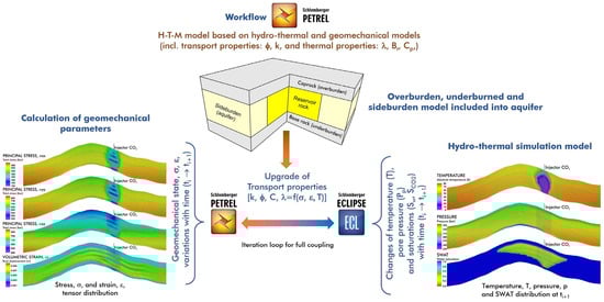
Figure 1.
The schematic illustration of the H-T-M coupling procedure applied to the dynamical model.
2.3. Evolution of Transport Properties
Under non-isothermal conditions, the spread of the injected fluid in the formation leads to an expansion of the cooled zone around the injection wells. After a certain time from the start of injection, the volume of the cooled rock is less than the volume already saturated with the injected fluid. This effect is directly proportional to the ratio between the heat capacity of the injection fluid and the reservoir rocks. As a result, this phenomenon leads to rapid changes in the geomechanical stability of the reservoir formation. In order to predict and study the plastic deformation of the rock caused by pressure and temperature changes, the geomechanical state is resolved in specific time steps. The magnitude of the changes in the elastic stiffness tensor and the associated changes in the stress () and strain () components are calculated on the basis of changes in pore pressure () and temperature (). According to the Kozeny–Carman model [63], the solutions related to the changes in the stiffness tensor, with particular attention to the evolution of the volumetric strain (), allow the quantification of the degree of changes in the transport properties (). The change in porosity () due to variations in volumetric strain () is first determined as shown in Equation (8):
The modified permeability () is then calculated directly from its initial value () by taking into account the original () and the modified porosity (), as shown in Equation (9):
As a result, the variations in the transport properties due to elastic deformations are spatially filled on the entire simulation grid. However, the influence of these deformations on the flow dynamics in the rock matrix is relatively small. The resulting permeability may not change significantly compared to the initial value, as the effects of the pressure increase and temperature decrease are not significant. If we consider the isothermal conditions in carbonate formations, the high injection pressures can induce elastic deformations that increase the permeability of the fractures by several orders of magnitude [27].
In naturally fractured reservoirs, the permeability of the fractures is the most important factor influencing the overall permeability. To determine the variation in fracture permeability under different geomechanical conditions, a stress-dependent model was adopted and modified according to the work of Min et al. [64] by combining the effects of normal and shear stress. In this work, a three-stage failure analysis was performed, which included continuous elastic deformations interrupted by plastic deformations such as fracture reactivation and rock failure. Plastic deformations can lead to rapid changes in fracture opening driven by dilatation mechanisms. The changes in fracture permeability () are then a function of the effective normal stress. The mechanism of elastic deformations has only a minor effect on the permeability, as at most a two-fold increase can be observed. The polynomial approximation of the permeability coefficient, which is defined as a function of the effective normal stress, was found based on the previously mentioned model from the literature [64], as shown in Equation (10):
Optimally oriented fractures are those that are more prone to early reactivation. Shear stress induces traction, which leads to a strong permeability response, but only to a limited extent. The observed decrease in effective normal stress below 14 MPa does not lead to a significant increase in permeability, which means that this parameter tends asymptotically to its maximum factor of 16. The limitation of this model is that new fractures are required to further increase the permeability of the rock due to its failure. The concept of predicting changes in the permeability of fractured rock due to reactivation of fractures and formation of new ones was loosely inspired by the modified Barton–Bandis model [65]. The conversion of the effective normal stress to the change in permeability associated with the reactivation of fractures () up to the reactivation limit is given by the following Equation (11):
If we consider the worst-case scenario, where the fractures are not optimally aligned, reactivation starts when the reaches 1.08 and drops from the original value of 30 MPa to −10 MPa. In fractured rock masses, failure occurs when the effective normal stress falls below −6 MPa. This is associated with the formation of new fractures and can also multiply the permeability () by the factor of 35. The relationship between the increase in permeability due to the failure of fractured rock and the opening of new fractures is shown in Equation (12):
Plastic deformation was hypothesized to be a major factor in increasing rock permeability, but it can also lead to the development of potential CO2 leakage pathways. The schematic plot of permeability variations concerning fractured rocks implemented in the coupled simulation model of the analyzed oil reservoir is shown in Figure 2.
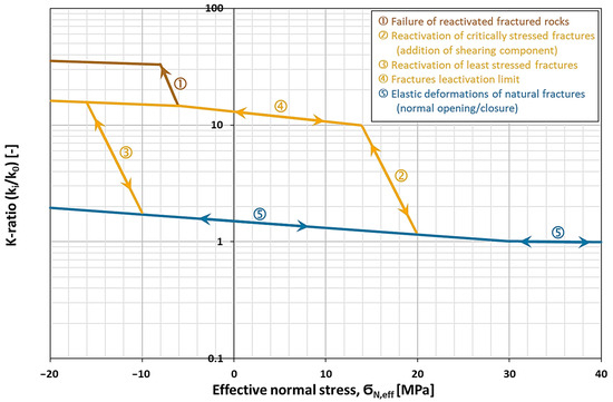
Figure 2.
Schematic relationships between the ratio of the increase in permeability () and the effective normal stress (). The brown line (1) determines a failure of fracture-prone rock masses with the formation of new fractures. The yellow curve (2) indicates the permeability route of critically stressed fractures during the reactivation process. The yellow curve (3) indicates the reactivation of fractures that are not optimally aligned. The yellow curve (4) marks the boundary of the reactivation mechanism of the fractures. The blue line (5) refers to the development of fracture permeability under elastic deformations.
3. Geological Modeling
Structural Modeling
The three-dimensional (3D) structural model of the studied oil field was created based on 3D seismic and well data, including geophysical logs and the results of a special core analysis. The integrated modeling process included the volume of the reservoir formation, supplemented by the overlying caprock and the underlying base rock (Figure 3). The geological model of the analyzed oil field structure was created and supplemented with reservoir properties and thermal and geomechanical parameters. The oil-saturated volume was mapped, taking into account the results of the interpretation of the 3D seismic data, calibrated with the well data, and finally, confirmed with the results of the DSTs and well tests. Based on the parametric model, the fluid flow simulations were initialized, executed, and adjusted to the history.
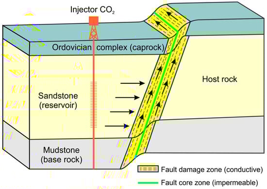
Figure 3.
Schematic of the structural model, including model zonation, dislocation, and leakage pathways. The intact host rock is separated by the fault zone, which is composed of two individual facies: an impermeable fault core and a highly conductive, naturally fractured damage zone. The potential CO2 leakage pathways are marked with black arrows.
The total number of grid blocks in the structural model is 1,522,248 (182 × 164 × 51), of which 410,363 are active. A static geologic model of the Middle Cambrian reservoir series was created with a fixed horizontal grid resolution of 75 × 75 m to match the available computational resources. The vertical resolution varied in the range of 1–3 m, with an average of about 1.50 m. The geological model covered a total thickness of about 70 m, of which about 40 m was the reservoir zone, about 15 m was the overburden, and about 15 m was the underlying strata. Water inflow rates were matched using a global grid approach at each well to within 2% of the error, and the total water production from the reservoir was balanced. Therefore, the construction of LGRs around individual wells was not mandatory in this case. In order to correctly reproduce the boundary conditions and reduce consumption of computational resources, including the lateral extent of the numerical aquifers, the horizontal extent of the model was limited to approximately 11.0 × 4.5 km.
The studied oil field is structurally sealed to the east by a fault zone. The western edge of the reservoir model is bounded by a linear no-flow zone mapped based on seismic data. These two sides of the structural model run parallel to each other in a north–south direction and are regarded as edges of the simulation model. However, the eastern fault zone is of regional importance. In the south, the studied oil field is bounded by the oil–water contact. As there are no direct measurements, the location of the northern boundary of the reservoir was approximated by analyzing seismic data in terms of seismic attributes and spectral decomposition. It was assumed that the northern boundary of the reservoir is facies-like. In this study, the classical approach of geological modeling of fault zone architecture was applied. Faults were implemented as part of a structural grid with an appropriate reduction in transmissibility between the blocks associated with the fault plane [66,67,68]. For the purposes of this study, the dislocation model was adopted based on data from the literature [69,70]. The conceptual model of dislocation used in this paper is shown in Figure 3. The chosen structural modeling approach enabled the explicit determination of the geomechanical stability of fault zones during the EOR process.
The structural model selected for this study assumes that the fault zone is divided into the barely permeable fault core and the conductive damage zone due to the occurrence of natural fractures [69]. The fault core is formed by the crushing of rock into a clay fraction and represents an effective barrier perpendicular to the direction of flow. The damage zone surrounding the fault core is a volume of rock traversed by a dense network of natural fractures that have developed close to the slip surface of the fault on both sides [70]. Therefore, the damage zone is characterized by increased permeability along the fault plane. The permeability of the damage zone in a direction perpendicular to the fault surface is usually lower, as most fractures are aligned with the main fault plane. The effectiveness of the fault zone system as a barrier was tested during the history-matching process. The results of history matching and division of the zones in the geological model are shown in Figure 4.
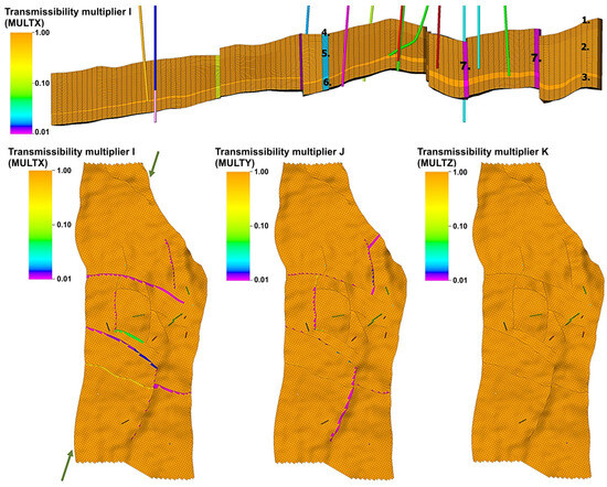
Figure 4.
Division of zones in the geological model. 1—caprock zone, 2—storage rock zone, 3—base rock zone, 4—caprock fault damage zone, 5—storage rock damage zone, 6—base rock fault damage zone, and 7—fault core zone. The green arrows indicate the cross-section line shown above in the figure.
The substantial model configuration related to parameter description is discussed in detail in the Appendix. The petrophysical, geothermal, and geomechanical properties are discussed in subsequent Appendix A, Appendix B and Appendix C. The geomechanical modeling, failure criterion, and boundary conditions for the geomechanical model are expanded in subsequent Appendix D, Appendix E and Appendix F.
4. Initialization of Hydro-Thermal Dynamic Model
The dynamic modeling was initialized based on an integrated oil reservoir model comprising geological, geothermal, and geomechanical models. The starting point of the dynamic modeling was the implementation of the required components representing the equilibrium state of the reservoir. Therefore, the properties of the dynamic model take into account the initial distributions of the reservoir fluids, the transport properties of the reservoir fluid, and the thermodynamic properties of the hydrocarbon fluid. The dynamic model was supported by consistent input data for the initial conditions, including pressure, temperature, and fluid saturation distributions. The initial formation pressure was determined based on DST measurements and well tests in accordance with a hydrostatic gradient of 0.0108 MPa/m and ranged from 23.0 MPa to 25.0 MPa, with an average value of 24.0 MPa. The spatial heat distribution was determined based on a surface temperature of 15 °C and a geothermal gradient of 0.0312 °C/m, calculated from borehole measurements. The resultant temperature ranged from 78 °C to 81 °C, with an average value of 80 °C. The spatial distribution of reservoir fluids was introduced to saturate the geologic structure with oil and water under conditions of hydrostatic equilibrium. In this study, the standard Corey model with a power approximation was used to predict the wetting and non-wetting multiphase flow, considering the following systems: water–oil, oil–CO2, water–CO2, as well as a trapping mechanism [71]. Corey curves were calibrated separately for each lithofacies to account for the heterogeneity of flow within the reservoir. Reduced saturations () were calculated using endpoint parameters (), as shown in Equation (13):
where —relative permeability, —reduced fluid saturation, —exponent, and —point parameters.
The dependence of the relative permeability coefficients on the reduced saturations is given by Equation (14):
The point parameters were inserted into the model according to data from the literature [72], and their values are given in Table 1.

Table 1.
Relative permeability curve parameters.
The realistic spatial distributions of the fluids in the oil reservoir were resolved using the hydrostatic equilibrium approach (J-function), according to Leverett [73] and assuming the initial absence of a gas cap. The subdivision into four facies zones was applied to the studied oil reservoir. It was supplemented by seventeen further regions in the central and eastern part of the reservoir, which were characterized by variable water wettability, and a northern region, which was associated with high water saturation. For the indicated regions, the procedure of fitting the Leverett J-function to the geophysical measurements of the water saturation profiles in boreholes was carried out. The general form of Leverett’s J-function was assumed according to Equation (15):
where —reduced water saturation, —permeability, —porosity, —capillary pressure for water–oil system, —capillary pressure for water–oil system (25 dyn/cm), and —contact angle for water–oil system (0°).
The thermodynamic model of the black oil reservoir (water and oil saturated with natural gas and CO2) was created using PVTSim software. The model was characterized by PVT correlations of a number of parameters for the defined fluid components, including density, viscosity, and solubility. The distributions of oil saturation (SOIL), pressure (PRES), and temperature (TEMP) for the initial state (t = 0) and the pre-injection phase (t = 10) are shown in Figure 5 in an exemplary vertical cross-section SW–NE.
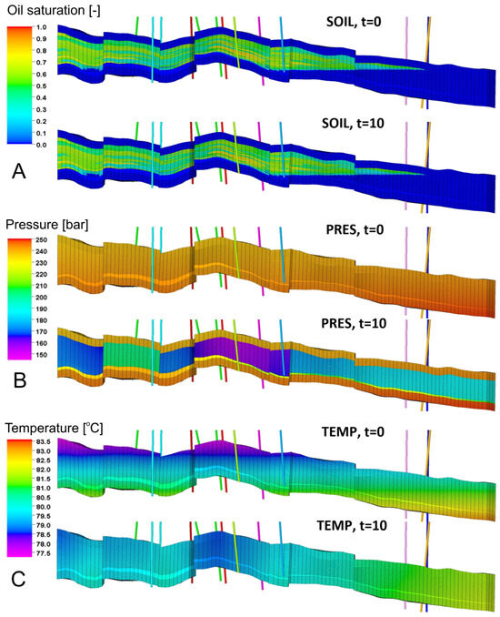
Figure 5.
The distributions of oil saturation (SOIL), pressure (PRES), and temperature (TEMP) for the initial state (t = 0) and the pre-injection phase (t = 10) on an exemplary vertical cross-section SW–NE. Exemplary cross-sections of oil saturation (A) pressure (B) and temperature (C).
As a boundary condition for the flow, two analytical aquifers of the Carter–Tracy type [74] were attached to the side walls of the dynamic model, namely in the north and in the south. The purpose of implementing an infinite-acting aquifer was to create a buffer zone outside the numeric model for the injected fluids during both IOR and EOR phases. This implementation significantly reduced the flow resistance around the injection wells and slowed the associated average reservoir pressure build-up, which was consistent with historical data. The boundaries of the dynamic model, including the top of the caprock and the bottom of the base rock, were considered as barriers preventing the flow of mass and energy.
In the base case, oil production is assumed to be supported by water flooding from the beginning of the reservoir production phase. Cold water is planned to be injected into the reservoir formation at an annual mass rate of 0.43 megatons/year using five wells over a 24-year period. In the alternative case, after eight years of water flooding, the method will be switched to EOR with continuous CO2 injection into two southern and one western well. It is planned to inject cold fluids (water and CO2) under non-isothermal conditions through five wells over a 24-year period, including 437 megatons/year of CO2 through two southern wells and one western well, and 755 tons/day of water through the northern well. Non-isothermal injection conditions are achieved by an initial temperature gradient in the reservoir and a constant injection temperature in the range of 35–80 °C.
The complete set of initial and boundary conditions, as well as the schematic geometry of a coupled dynamic model, are shown in Figure 6.
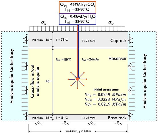
Figure 6.
The scheme with the initial properties, the boundary conditions, and the geometry of the geomechanical model. Orange and blue arrows indicate the directions of spread of the injected fluid.
5. Results Analysis
The numerical procedure was performed using the common structural mesh of the integrated HTM model. Fluid and heat flow simulations were combined with geomechanical state calculations to effectively predict the behavior of the offshore oil reservoir, including the evolution of transport properties caused by PT changes during the EOR process. All simulations that were performed considered realistic non-isothermal scenarios where the temperature of the injected fluid was lower than the reservoir temperature (), except the isothermal base case. The simulation results were documented for all specified time steps.
5.1. Waterflooding and EOR-CO2 Injection Assumptions
In the waterflooding simulation scenarios, water was injected through four wells at a rate adapted to the local transport properties of the reservoir. In the simulation variants related to CO2-EOR, injection was performed by a combination of a single waterflooding well in the north and three CO2 injection wells in the south. For both types of scenarios, the effect of oil sweep was tracked for 35 years, 18 years in the past and 16 years in the forecast. The main objective of the alternative injection program was to investigate the effect of the type of injection fluid on the total oil production of the field. In this work, the relaxation phase was not taken into account, so that the reservoir did not reach the HTM equilibrium state at the end of the simulated period. The IOR/EOR operations were controlled by the results of the geomechanical stability analysis. The standard protocol, which assumed formation stability, was changed when the top of the reservoir caprock failed and the injected gas was able to breach the caprock. Such an event was interpreted as a leak in the geologic structure of the oil reservoir and an inability to continue the IOR/EOR process.
The different operating assumptions were necessary to emphasize the thermal effects that influence the geomechanical stability of the selected oil reservoir. The production wells were controlled by a downhole pressure restriction of 100 bar to maintain the target oil production rates. Injection was performed over the entire interval of the reservoir formation to avoid the problem of increased injection pressure due to the flow resistance of the formation. The maximum wellhead pressure was set at 400 bar, which was intended to prevent excessive fracturing of the rock formations due to the applied overpressure. The maximum injection rate of the group was set at 1.1E6 sm3/d due to the technical capabilities of the waterflooding system. The minimum downhole temperature of the injection fluid was set above 30 °C () to ensure supercritical conditions of CO2 flow during injection and to minimize the risk of CO2 hydrate blockages.
Examples of pressure, temperature, and fluid saturation distributions for the initial state and after 10, 15, 20, 25, 30, and 35 years of the exploitation cycle of the oil reservoir are shown in Figure 7, Figure 8 and Figure 9.
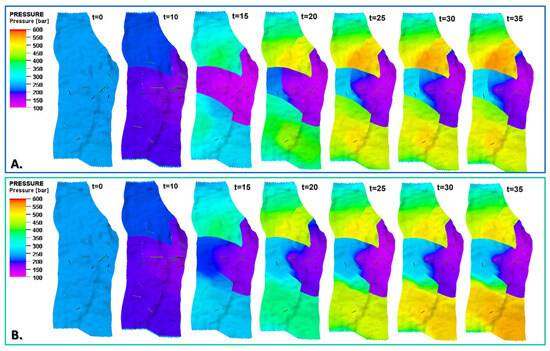
Figure 7.
Examples of pressure distributions for the initial state and 10, 15, 20, 25, 30, and 35 years of exploitation of the oil reservoir using IOR/EOR methods, including water flooding (A) and water–CO2 injection (B). Middle layer of reservoir model (K = 30).
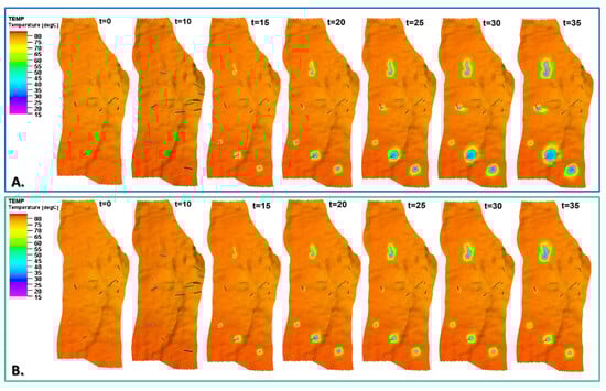
Figure 8.
Examples of temperature distributions for the initial state and 10, 15, 20, 25, 30, and 35 years of exploitation of the oil reservoir using IOR/EOR methods, including water flooding (A) and water–CO2 injection (B). Middle layer of reservoir model (K = 30).
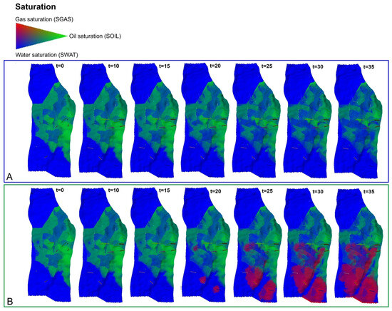
Figure 9.
Examples of fluid saturation distributions (water—blue, oil—green, and CO2—red) for the initial state and 10, 15, 20, 25, 30, and 35 years of exploitation of the oil reservoir using IOR/EOR methods, including water flooding (A) and water–CO2 injection (B). Middle layer of reservoir model (K = 30).
5.2. Analysis of Coupled HTM Simulations
To maximize EOR enhanced oil production by creating an optimal oil displacement front, a configuration of peripheral injection wells was designed. The irregularity of the oil displacement front is consistent with the anisotropy of the reservoir formation’s transport properties, as shown in a comparison of Figure 2 and Figure 4. In some areas of the formation, the extent of oil displacement relative to the size of the CO2 plume is structurally constrained by both sealing faults and small-scale faults within the formation. In contrast to the expansion of the volume occupied by the injected fluids in the reservoir, symmetry is also observed in the spread of the cooled zone in all horizontal directions. The maximum lateral extent of the cooled zone (after 35 years) was three times greater in cases with waterflooding than in the EOR-CO2 scenarios, as shown in Figure 8. An exception to this rule can occur if the injection well is located close to the conductive fault. This situation was observed for the injection well in the north (XI-4). As a result, the oil displacement front and the cooled zone expanded rapidly along the fault zone during the first year of the EOR process. In this particular case, unlike the rock volume occupied by the injected water, the cooled zone could not extend far beyond the fault zone. The observed phenomenon of fault cooling is a negative symptom related to maintaining the tightness of the caprock. For this reason, the scenario of CO2 injection through a borehole in the north was not taken into account in the integrated simulation model.
6. Analysis of the Geomechanical Stability of the Oil Reservoir Structure
The main topic of this article is the evaluation of the geomechanical stability of the studied oil reservoir structure during IOR/EOR-supported oil production. In this context, questions regarding the influence of temperature and pressure on the resulting stress and strain state, as well as mapping the occurrence of rock failure, were raised. In addition to the geomechanical analysis, the elastic strain distributions were also investigated in order to determine the magnitude of changes in the transport properties of intact rock. In the model zones where the Mohr–Coulomb failure criterion was met, a corresponding flag was set for the reactivation or failure event. The author studied five non-isothermal cases (), as shown in Table 2, to verify reservoir stability and caprock tightness. For the most realistic case (), an additional detailed geomechanical analysis was performed, supplemented by Mohr circle diagrams for each stage of oil production supported by the EOR process.
Table 2.
List of simulation scenarios and general geomechanical stability results for injection zones.
6.1. Preliminary Results of the Geomechanical State and Stability
The spatial distribution of the diagonal components of both the stress and strain tensors in the zones close to the borehole after the start of the injection process is not uniform. The superposition of poroelastic and thermoelastic effects in the structure of the oil reservoir leads to a considerable change in the geomechanical state compared to the initial conditions. The development of these changes most likely correlates with the increase in the volume occupied by the cooled zone. The application of fluid injection at temperatures far below the formation temperature () leads to a strong thermoelastic unloading of both horizontal stress components () around the injection wells, as documented in Figure 10 and Figure 11. At the end of the well test phase (the first 10 years), a slight decrease in vertical stresses () can be observed in the central part of the reservoir, which is due to partial depletion. However, in the EOR phase (after the 10th year), the injection of cold water or scCO2 has no significant effect on the vertical stress component, as can be seen in Figure 12.
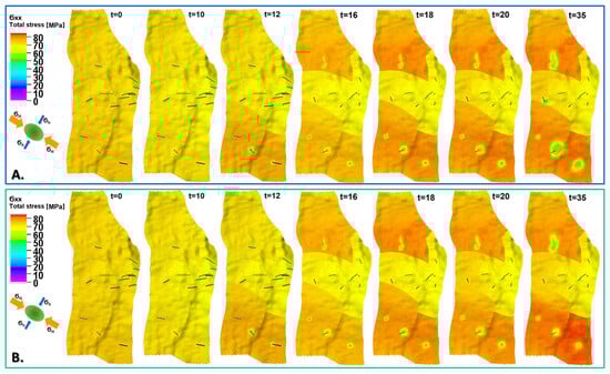
Figure 10.
Exemplary distributions of horizontal stress component () for initial state and 1, 10, 15, 20, 25, 30, and 35 years of oil production with EOR, including water injection (A) and water–CO2 injection (B). Middle layer of reservoir model (K = 30).
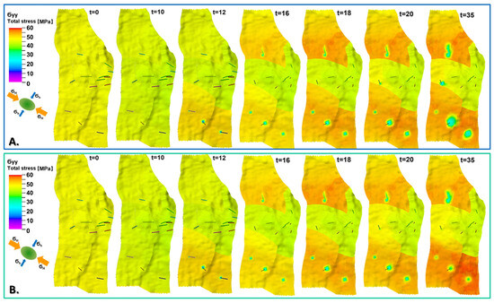
Figure 11.
Exemplary distributions of horizontal stress component () for initial state and 1, 10, 15, 20, 25, 30, and 35 years of oil production with EOR, including water injection (A) and water–CO2 injection (B). Middle layer of reservoir model (K = 30).
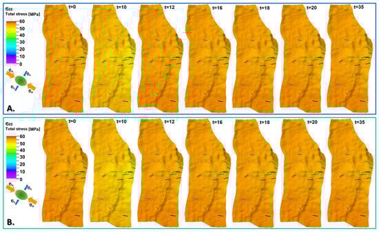
Figure 12.
Exemplary distributions of vertical stress component () for initial state and 1, 10, 15, 20, 25, 30, and 35 years of oil production with EOR, including water injection (A) and water–CO2 injection (B). Middle layer of reservoir model (K = 30).
The propagation of the cooled zone also led to a local decrease in the magnitudes of the horizontal diagonal components of the strain tensor () in the central part of the model. This is observed mainly in the layers with higher porosity of the geological model due to the more pronounced contraction of the sandstone lithology with decreasing temperature. A similar negative effect to that described above can be observed for the volumetric strain in Figure 13. However, the positive deformation effects in the aquifers surrounding the injection zones are relatively weak (). The negative thermoelastic effects cause a significant compensation of the deformations in the zones around the injection wells ().
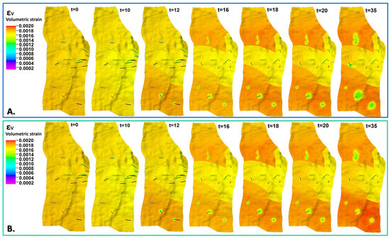
Figure 13.
Exemplary distributions of volumetric strain () for initial state and 1, 10, 15, 20, 25, 30, and 35 years of the production with EOR, including water injection (A) and water–CO2 injection (B). Middle layer of reservoir model (K = 30).
Thermoelastic-induced stress unloading causes a rotation of the original stress tensor, which is accompanied by a rapid transition from the strike-slip stress (SS) regime to the normal fault (NF) regime. The local extent of the occurrence of the NF stress regime can be seen in Figure 14. The observed change in stress state can have a significant impact on the failure mode and the kinetics of the induced dislocation movements. The compressive strike-slip regime favors the reactivation of critically stressed fractures or the development of shear fractures within the reservoir formation and caprock during horizontal displacement. The area affected by a normal faulting stress regime is more prone to the development of tensile fractures or the reopening of existing discontinuities with accompanying vertical rock displacements.
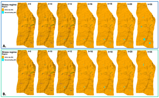
Figure 14.
Exemplary distributions of stress regime, orange—strike-slip () or blue—normal faulting (), for initial state and 1, 10, 15, 20, 25, 30, and 35 years of oil production with EOR, including water injection (A) and water–CO2 injection (B). Middle layer of reservoir model (K = 30).
Any type of rock failure would have a significant impact on the flow conditions in the structure of the oil reservoir, as already described in Figure 2. Furthermore, damage to the overburden may result in the reservoir no longer being leak-tight, as potential CO2 escape paths through the overburden will be created. The modeled temperature drop near the injection wells leads to a rapid failure of the rock in tensile mode, accompanied by the reopening of existing natural fractures. In the scenarios with waterflooding, the extent of the tensile failure zone increases as the IOR process progresses, as does the extent of the cooled zone. Compared to the EOR-CO2 scenarios, the reservoir formation becomes more stable and the volume occupied by damaged rock decreases, as shown in Figure 15. The process of reactivation of natural fractures follows the directions of the reservoir volume affected by rock failure, but over a much larger area. For example, the area reactivated by the temperature drop thus surrounds the volume of the failed rock around the injection wells. The overpressure-induced reactivation of fractures occurs near the injection wells, mainly north of the southern wells (XI-1, XI-2) and to a lesser extent north of the northern well (XI-4). The failure of the rock in tensile mode increased the permeability of the zones near the injection wells, which led to a decrease in injection pressure due to the decrease in the flow resistance of the formation. The observed geomechanical response of the oil reservoir is consistent with the recorded events in the production history, particularly the accelerated water breakthrough from the south into the XP-4 production well and the increased communication with the aquifers through the reactivated zones.
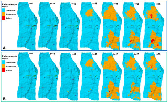
Figure 15.
Exemplary distributions of failure mode, blue—stable formation, orange—fracture reactivation, and red—rock shear/tensile failure, for initial state and 1, 10, 15, 20, 25, 30, and 35 years of the oil production with EORs, including water injection (A) and water–CO2 injection (B). Middle layer of reservoir model (K = 30).
The geomechanical stability analysis was based on the Coulomb–Mohr failure criterion, taking into account the plasticity function. Based on this assumption, the reservoir formation remained stable during the first nine years of the well-testing phase. The first occurrence of conditions favorable for the reactivation of fractures was observed in the fourth year of the EOR phase in the reservoir interval of all four injection wells (XI-1, XI-2, XI-3, and XI-4). The reactivated area increases as the EOR phase progresses. The reactivation process involves the sealing layers of the underlying base rock, from the eighth and tenth year of injection in the case of injection wells XI-2 and XI-1, with XI-4. Since the start of injection (fourth year of EOR), fractures in the reservoir interval near the XI-4 well were rapidly reactivated by transitioning into the basement and the damage zone of the nearby fault. After eight years of EOR, the entire modeled interval in this well is reactivated, except for the caprock, including the reservoir, base rock, and adjacent fault damage zone. Well XI-3 to the south was the least susceptible to reactivation due to the cessation of injection in the tenth year of EOR. In that well, reactivation only affected the zones near the wellbore in the reservoir interval since the eighth year of the EOR phase. In the case of the western hinge of the reservoir, the area around well XI-5 was not reactivated. The reactivation process mainly affects stiff lithologies, where the probability of natural fracture occurrence is higher, including the reservoir interval where fractures have been observed on borehole images. After 8 years of injection, the accumulation of compressive stresses caused by the increase in pore pressure leads to the formation of an extensive reactivation zone located outside the drilling zones of the southern injection wells in a radius of up to 1 km to the north. This phenomenon can be explained by the increased conductivity of the fractures for the water injected from the south and is related to the observed rapid increase in water production at well XP-4. Since there are no measurements, it is still a matter of debate whether there are natural fractures in the overlying carbonates. Small-scale calcite-healed fractures were found in only one core sample from the caprock at the offset well. In this study, it was assumed that there are pre-existing natural fractures in the caprock. Consequently, the structure of the oil reservoir will lose its integrity if the reactivation or failure zone develops simultaneously in the reservoir and the overburden.
The failure zone appears after the first year of the EOR phase in the most vulnerable reservoir interval of the two wells, XI-1 and XI-2, in the south. In these wells, the failure zone never extends beyond the reactivation zone and spreads in all directions, similarly to the reactivated area. Since the sixth year of EOR, the failure zone has been observed at the reservoir interval of the three boreholes XI-1, XI-2, and XI-4. The same situation occurs in the tenth year of the EOR phase at the well XI-3. At the end of the simulated time interval (after 35 years), the failure zone reaches 210 and 350 m from the injection wells XI-2 and XI-1, respectively. This horizontal extent of the failed rock correlates with a very pronounced negative horizontal thermoelastic effect due to the injected cold water (). After seven years of the waterflooding phase, numerous rock failure events were observed around the two southern injection wells (XI-1 and XI-2). The same situation occurred in the northern injection well (XI-4) after nine years of water injection. These events were not able to trigger the upward leakage paths of the injection fluid in the prediction scenarios. The results of the preliminary geomechanical stability analysis performed for the water injection case and related to the classical C-M criterion are presented in Table 3 for comparison purposes.
Table 3.
Results of geomechanical stability analysis performed according to Coulomb–Mohr (C-M) failure criterion for selected oil production with IOR-waterflooding. Reactiv.—fracture reactivation event, FM_S—rock failure in shear mode, FM_T—rock failure in tensile mode, Leak (NO/Up)—no observed CO2 leakage/upward leakage through specific region, 1, 2, 3, 4, 5, and 6—numbers of regions determined in dynamic model enlisted in Figure 6, and NO—formation is stable.
During CO2 injection into the southern wells (XI-1 and XI-2), the area of the failure zone stabilizes and remains constant throughout the forecast period, with the radius in both wells reaching approximately 200 m. Thermal effects also contribute to the rapid failure of the reservoir rock several years after the start of injection in well XI-4. In the sixth year of injection, the failure spreads to the damage zone of the nearby fault. Furthermore, since the eighth year of EOR, the entire modeled section of borehole XI-4 is covered by the reactivation zone, separated by intervals of failed rock. In the southwest, the failure zone occurs only in the vicinity of injection well XI-3, between the seventh and ninth year of the EOR phase. The failure is not observed at the XI-5 injection well, because water is injected into the depleted zone in the western part of the reservoir. The switch to scCO2 injection in most wells from the eighth year of production leads to an increase in the overall horizontal permeability of the reservoir interval due to a lower cooling effect of CO2 on the rocks and, consequently, to a more pronounced extension of the reactivation zone. However, the failure zone does not propagate upwards during the forecast, and the integrity of the caprock is maintained, so no leakage of the injected fluid is observed. The results of the preliminary geomechanical stability analysis performed for the scCO2 injection case and related to the classical C-M criterion are presented in Table 4 for comparison purposes.
Table 4.
Results of geomechanical stability analysis performed according to Coulomb–Mohr (C-M) failure criterion for selected oil production with EOR-CO2. Reactiv.—fracture reactivation event, FM_S—rock failure in shear mode, FM_T—rock failure in tensile mode, Leak (NO/Up)—no observed CO2 leakage/upward leakage through specific region, 1, 2, 3, and 4—numbers of regions determined in the dynamic model enlisted in Figure 6, and NO—formation is stable.
6.2. Analysis of the Impact of Poroelastic and Thermoelastic Effects
To establish the relationship that describes the influence of pore pressure and temperature variations in the reservoir () on the principal components of the stress tensor (), the relative changes in pore pressure and temperature (), as well as the relative changes in the stress tensor component (), must first be determined. As can be seen from Figure 16 and Figure 17, the thermal stress caused by temperature changes is, on average, more than twice as large as the effect of the pore pressure on the horizontal stress components. In addition, the superposition of the thermoelastic and poroelastic effects reduces the vertical stress component to practically zero. These two effects lead to modifications of the stress–strain tensor, especially its horizontal components, resulting in drastic changes in the geomechanical stability of the oil reservoir structure. As a result, the transport properties of the reservoir formation evolve together with the changes in the geomechanical state. Shortly after the start of the IOR waterflooding phase, and continuing during the EOR-CO2 phase, the thermoelastic effects exceed the poroelastic effects three-fold in the near-wellbore zones where cold fluid has been injected. As a result, the magnitudes of the horizontal stress components decrease rapidly compared to the initial state. After several years of continuous injection of cold water, a decrease in the ratio of thermal stress to poroelastic stress () to 1.7 can be observed, which is due to the pressure build-up.
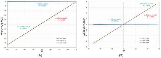
Figure 16.
The contribution of temperature () and pressure () fluctuations to the change in the principal components of the stress tensor, (A) and (B) .
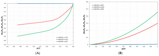
Figure 17.
The relationship between the relative change in temperature () and pressure () to the relative change in the principal components of the stress tensor, (A) and (B) .
In general, the resulting relative changes in the vertical stress component () are negligible (−0.0021, 0.0023) due to the mutual compensation of temperature and pressure effects. Moreover, the relative change in vertical stress caused by the relative change in pressure () is seven times greater than that caused by the relative change in temperature. It can be concluded that the greatest influence of the relative change in temperature () on the relative change in the horizontal components of the stress tensor () is observed shortly after the start of injection (). As the injection approaches the minimum target temperature, the relative change in the horizontal components of the stress tensor reaches a minimum value (). At the end of the first year of the injection phase, the relative change in pressure reaches a value of 0.32, resulting in a relative change in the horizontal stress components of 0.08 on average. After the EOR phase, the relative change in pressure reaches a maximum value of 0.53, which corresponds to a relative change in the horizontal stress components of 0.15.
The correlations described above represent a certain average trend of changes occurring in the blocks of the simulation model. It should be noted here that the observed anisotropy of the properties of the reservoir rocks suggests that different relationships should be determined for each block of the model. These relationships may have a larger spread, but they would be centered around the curves shown in Figure 16. The nonlinearity of the impact of temperature on the resultant stress tensor, shown in Figure 17, in the case of CO2 injection, additionally makes it difficult to easily describe and predict the results of thermoelastic phenomena on the reservoir rocks. An easier case to describe is the effect of pressure on the resultant stress tensor; this relationship is also nonlinear but with a smoother course.
6.3. Detailed Analysis of Geomechanical Stability
In this work, an analysis of the change in the stress state and the geomechanical stability of the reservoir was also carried out using Mohr’s circle diagrams. The analysis refers to the blocks of the oil reservoir model where the strongest changes in stress state occurred and where the highest probability of leakage in the structure of the oil reservoir was identified. These include areas that have been previously plasticized, mainly due to strong temperature changes, i.e., near the well that is injecting the cold fluid, in the fault zone (damage zone). The detailed analysis was performed for two variants that differed in the type of injected fluid, but in both cases, the minimal injection temperature was constant, i.e., 35 °C. The central depleted part of the reservoir, where the oil production takes place, is where the reservoir formation remains stable throughout the entire operational life of the reservoir. Figure 18, Figure 19 and Figure 20 are introduced generally to be combined with Figure 21 and Figure 22 and to complement the detailed stability analysis. These figures were introduced to follow stress evolution trends at sample locations of high deviatoric stress through the exemplary time points to find stability loss events simultaneously on vertical sections and Mohr’s circle diagrams. The most important here are the key points relating to reactivation (RE) and failure in shear, hybrid, or tensile modes (SF, HF, and TF). These events are depicted in Figure 21 and Figure 22 and in the above mentioned discussion to emphasize their importance in enhancing the transport properties of the reservoir formation or opening potential escape routes for CO2.
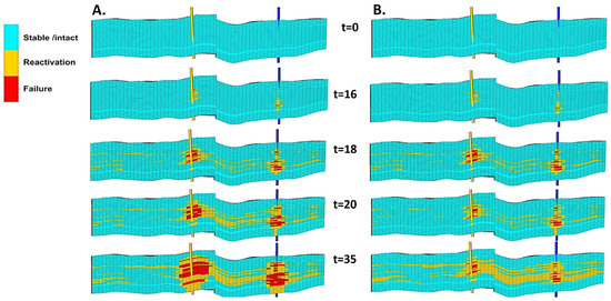
Figure 18.
The geomechanical stability analysis of the selected oil reservoir (well XI-1 and XI-2) in terms of the Coulomb–Mohr approach with respect to plasticity function. Vertical cross-section between XI-1 (yellow) and XI-2 (indigo) injection wells. Non-isothermal scenario () for the following 0, 16, 18, 20, and 35 years of the oil production with EOR, including water injection (A) and water–CO2 injection (B). Failure mode: blue—stable/intact formation, yellow—reactivation, and red—failure. Color lines represent production and injection wells.
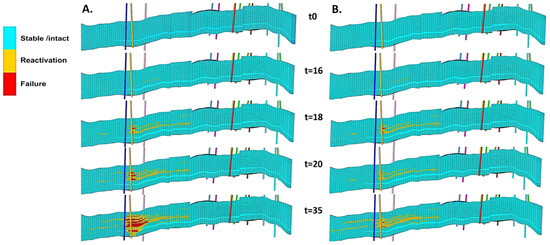
Figure 19.
The geomechanical stability analysis of the selected oil reservoir (well XI-1) in terms of the Coulomb–Mohr approach with respect to plasticity function. Vertical cross-section between XI-1 (yellow) injection well in the south and the northern part of the reservoir. Non-isothermal scenario () for the following 0, 16, 18, 20, and 35 years of the oil production with EOR, including water injection (A) and water–CO2 injection (B). Failure mode: blue—stable/intact formation, yellow—reactivation, and red—failure. Color lines represent production and injection wells.
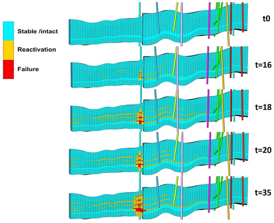
Figure 20.
The geomechanical stability analysis of the selected oil reservoir (well XI-4) in terms of the Coulomb–Mohr approach with respect to the plasticity function. Vertical cross-section between XI-4 (blue) injection well and the north-eastern part of the reservoir. Non-isothermal scenario () for the following 0, 16, 18, 20, and 35 years of the oil production with EOR, including only water injection. Failure mode: blue—stable/intact formation, yellow—reactivation, and red—failure. Color lines represent production and injection wells.
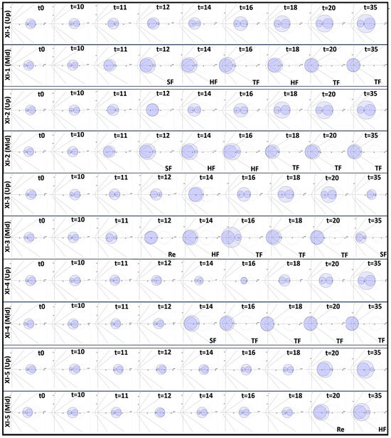
Figure 21.
The geomechanical stability analysis of the selected oil reservoir (well XI-1, XI-2, XI-3, XI-4, and XI-5) in terms of the Coulomb–Mohr approach with respect to plasticity function. Up—uppermost layer of caprock and Mid—middle layer of reservoir formation. Non-isothermal scenario (), for the following 10, 11, 12, 14, 16, 18, 20, and 35 years of production and waterflooding stage. Re—reactivation of pre-existing fractures, SF—shear failure, HF—hybrid failure, and TF—tensile failure.
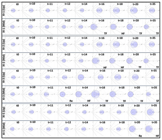
Figure 22.
The geomechanical stability analysis of the selected oil reservoir (well XI-1, XI-2, XI-3, and XI-5) in terms of the Coulomb–Mohr approach with respect to plasticity function. Up—uppermost layer of caprock and Mid—middle layer of reservoir formation. Non-isothermal scenario (), for the following 10, 11, 12, 14, 16, 18, 20, and 35 years of production and EOR-CO2 stage. Re—reactivation of pre-existing fractures, SF—shear failure, HF—hybrid failure, and TF—tensile failure.
According to the result presented in Table 2, if we consider isothermal conditions (base case) and in most non-isothermal cases (), only critically stressed fractures are favorable to reactivate in the area of several hundred meters around the injection wells, mainly due to applied overpressure. When the EOR process advances and the temperature difference increases below −30 °C, thermoelastic stresses produce conditions favorable to tensile failure, but exclusively in the zones near the injection wells. As the temperature of the injected fluid approaches its minimum value (), there is an early decrease in the average, resulting in both horizontal stress components (), from about 3% at 70 °C to a maximum of 74% and 78% at 35 °C. These large changes in the two horizontal components of the stress tensor () coincide with the predominant directions of cold fluid flow through the sequestration structure, i.e., along the meridional axis of the structure, and perpendicular to it. In the individual injection wells, such a decrease occurs at different times, e.g., in the southern wells after 11 years and in the northern well after 14 years from the start of the reservoir life cycle. The vertical component of the stress () does not change significantly during the entire simulated period (35 years). For this reason, the continuous cooling of the zones near the injection wells leads to a transition from the strike-slip stress regime (SS) to the normal faulting regime (NF). The increase in differential stresses creates optimal conditions for the reactivation of critically stressed natural fractures or directly causes a failure in shear, hybrid, or tensile modes. In the case of the zone around the south-eastern well (XI-2), the natural fractures are reactivated very quickly in the middle interval of the reservoir during the first year of water injection. Shear failure occurs one year later, and during the next five years the middle interval of XI-2 well switches to hybrid failure. Tensile failure conditions persist until the end of the forecast, as shown in Figure 18. The change in injection fluid from water to scCO2 (year 18) also leads to a continuation of the stress failure conditions, but with a smaller opening of the hydraulic fractures, as seen by comparing the Mohr diagrams in Figure 21 and Figure 22. The near-well zone of the next southern well (XI-1) is subject to a similar development of the stress state. The difference is that a stress failure occurs in a wider zone around this well. After year 16, well XI-1 is under tensile failure conditions, but two years later, there is a slight relaxation due to reduced average injection rates, and the near-well zone re-enters a hybrid failure condition. This condition does not last long, because from year 19 until the end of the forecast, tensile failure conditions are mainly observed in the most unstable layers. The change from water injection to scCO2 (year 19) leads to continued tensile failure conditions but causes smaller hydraulic fracture openings. The development of the changes in the stress state for wells XI-1 and XI-2 can be seen in Figure 15, Figure 18, and Figure 19. The zone around the south-western well (XI-3) remains stable until year 11, and from year 12 it is mostly reactivated with a single interval under shear failure conditions. After year 14, the near-well zone is under hybrid failure. From year 16 to the end of the history (year 19), tensile failure conditions prevail, with a decreasing aperture of hydraulic fractures. From year 20 to the end of the forecast (year 35), there is a period of incomplete relaxation caused by well abandonment, during which a gradual transition to shear failure occurs. The evolution of geomechanical changes in the vicinity of borehole XI-3 can be followed in Figure 21 and Figure 22. The development of the changes in geomechanical stability of the northern wells differs from the southern ones, e.g., because they started injecting a half-year later, when the conditions in the reservoir were different than at the beginning. In the case of the northern well (XI-4), the near-well zone remains stable until year 13. In the following years, the natural fractures are reactivated, including the adjacent small fault to the northeast. From year 14, a shear failure occurs, which quickly turns into a tensile failure (from year 16 to 35). The development of the failure of XI-4 is shown in Figure 20. The north-western well XI-5 remains stable until year 19 due to a late connection to the injection system. Since year 20, the unstable layers enter reactivation mode but gradually move towards a shear and hybrid failure mode until the end of the forecast. The caprock layers above the interval provided for the injection remain stable throughout the simulated history and forecast, demonstrating their sealing capacity in the waterflooding and EOR-CO2 process, as can be observed in Figure 21 and Figure 22.
Figure 21 and Figure 22 are introduced generally to be combined with Figure 18, Figure 19 and Figure 20 and to complement the detailed stability analysis. These Figures were introduced to follow stress evolution trends at sample locations of high deviatoric stress through the exemplary time points to find stability loss events simultaneously on vertical sections and Mohr’s circle diagrams. The most important here are the key points relating to reactivation (RE) and failure in shear, hybrid, or tensile modes (SF, HF, and TF). These events are depicted in Figure 21 and Figure 22 and in the previously mentioned discussion to emphasize their importance in enhancing the transport properties of the reservoir formation or opening potential escape routes for CO2.
Considering the results described in Section 5.1, an increase in the deviatoric effective stress can result in a significant increase in long-term permeability due to natural fracture reactivation or rock failure. A decrease in the effective stress to a level below 20 MPa can trigger fracture reactivation, leading to a ten- to sixteen-fold increase in permeability. If the decrease in effective stress below −5 MPa is associated with rock failure, the permeability can reach a factor of 35. Changes in permeability in intact rock due to elastic deformation and induced by temperature drop are considered to be a relatively weak factor due to their small magnitude (up to a two-fold increase). As mentioned earlier, the assessment of geomechanical stability is crucial because only inelastic deformations are able to significantly change the transport properties of the formation or increase the risk of loss of caprock integrity.
7. Summary and Conclusions
The research work described in this article deals with the analysis of the geomechanical stability of an oil reservoir during its production cycle, taking into account secondary (IOR-waterflooding) and tertiary (EOR-CO2) methods. During the injection of water and CO2 at a temperature much lower than the reservoir temperature, significant shear and tensile stresses were generated. The study focused on the practical issue of reservoir and caprock integrity, taking into account thermo-poroelastic effects. This paper is a summary of the presented research. Among other things, it contains assumptions, the numerical method used, and conclusions proving the validity of the selected production IOR and EOR methods. The analyses carried out enabled an attempt to optimize the production conditions of the oil reservoir with regard to the failure that occurred and to formulate conclusions from these analyses. As a result of performing the above tasks, the following conclusions were formulated as bullet points:
- (1)
- The quality of the geomechanical model was significantly improved by calibrating in-situ stress to the results of production test, injection tests, and mini-fracs.
- (2)
- A detailed geomechanical analysis with Mohr diagrams was performed exclusively for the most stressed areas of the oil reservoir, i.e., the zones around the injection wells and in the overburden layers above these wells.
- (3)
- The geomechanical calculations and heat flow simulations took into account the changes in the thermal, geomechanical, and transport properties of the reservoir rock due to the effects of temperature.
- (4)
- The injection of cold fluids (water and CO2) into hot reservoir rock leads to a significant change in the initial stress tensor, mainly in the vicinity of the injection wells.
- (5)
- The cooling of the fault zones and the zones around the injection wells, as well as the temperature drop in the lower part of the caprock due to thermal conduction, leads to a transition from the strike-slip stress regime to normal faulting conditions. Transition to a normal faulting regime is risky and may lead to the initiation of tensile failure. The effect is more pronounced when cold water is injected rather than scCO2.
- (6)
- The thermoelastic unloading in the reservoir leads to a significant reduction in the horizontal components of the stress tensor, while the vertical stresses remain practically unchanged (ΔσH = −47 MPa and ΔσV = −7 MPa for ΔTinj = −45 °C).
- (7)
- The contribution of the thermoelastic component is more than twice as large as that of the poroelastic component to the overall change in the horizontal components of the stress tensor, which was presented in Section 6.2 in Figure 16 and Figure 17. For this reason, thermal stresses should always be considered when the change in the formation temperature exceeds 10 °C.
- (8)
- The primary factor for the growth of fractures is the thermal drawdown, as a result of increasing tensile stresses with decreasing temperature. The secondary factors are the azimuth of maximum horizontal stress (WNW-ESE) as well as the magnitude of vertical stress.
- (9)
- It has been found that higher injected fluid temperature (above 35 °C), especially in the case of scCO2, can reduce or stop the hydraulic fracture opening mechanism due to lower tensile stresses, as shown in Section 6.3 in Figure 21 and Figure 22.
- (10)
- It has been estimated that changes in the geomechanical state of the oil reservoir can increase the formation permeability by sixteen times (fracture reactivation) to as much as thirty-five times (tensile failure).
- (11)
- Switching injection fluid from water to scCO2 may reduce the likelihood of premature breakthrough of the injected water into the production wells and also prevent reactivation of critically stressed fractures in the caprock.
- (12)
- It should be emphasized that the phenomenon of tensile stress accumulation in the overburden may lead to the generation of leakage pathways, but in the case of the selected offshore reservoir overburden, they remained stable throughout the simulated period.
- (13)
- The conducted hydro-thermo-mechanical (HTM) coupled simulation proved its effectiveness in the field of time optimization. A single coupled time step period duration was about ten seconds, and the total elapsed time of the coupled simulations was extended by less than 1%.
- (14)
- The enhanced oil recovery supported by CO2 injection (EOR-CO2) should be conducted by maintaining the supercritical conditions of downhole CO2 (80 bar > Pinj < 600 bar, 31 °C > Tinj > 80 °C). Such an approach guarantees the stability of the caprock throughout the whole prediction period.
Funding
This research was carried out as part of the project: “Geomechanical stability during CO2 sequestration process, exemplified by a selected oil field”, which is funded by the Polish Ministry of Science and Higher Education, Grant No. DK-4100-11/24. The author would like to express their gratitude to the Polish Ministry of Science and Higher Education for funding this research.
Data Availability Statement
Further inquiries can be directed to the corresponding author (part of the data are not publicly available due to confidentiality restrictions).
Conflicts of Interest
The author declares no conflict of interest.
Appendix A
Petrophysical Properties
Modeling of petrophysical properties was based on 3D seismic data supported by well interpretation results from 17 wells within the reservoir and 1 adjacent well. The parametric model was created by applying geostatistical methods to determine the distribution of facies, porosity, clay content, and net-to-gross ratio for the entire volume of the reservoir structure. For the parametric modeling, a method based on the stochastic algorithm of Gaussian random function simulation was used. The applied numerical procedure requires the determination of the variability range and the median values, including the modeling of the semivariogram of the investigated parameters. The final distributions of the modeled parameters were selected as the most probable statistical realization P50 of the uncertainty analysis, taking into account the co-kriging procedure to maintain fixed, upscaled values for the blocks associated with the wells.
In the first step, the facies profiles at the boreholes were reinterpreted. As a result, six new facies types were determined, including four types for the reservoir series and two for the sealing layers of the caprock and base rock. The reservoir interval consists of laminated sandstones with intraclasts, sand–mudstone heteroliths, massive sandstones, and mud–mudstone heteroliths. The caprock consists of a clay–carbonate complex, and the base rock is represented by underlying mudstones. In the second step, a custom parametric modeling algorithm was developed to link the 3D seismic records to the well data using Petrel workflows. The well-log porosity and the amplitude record of the 3D seismic image were correlated to determine a meta-attribute for pseudo-porosity, taking into account the genetic inversion of porosity and the seismic attributes. The resulting meta-attribute for pseudo-porosity was used to determine the facies distribution. Based on the propagating facies in the volume of the geological model, the effective porosity distribution was determined. The data obtained allowed the calculation of other necessary reservoir parameters, including permeability, clay content meta-attribute, and net-to-gross ratio, distributed on the regional grid of the geologic model. Permeability distributions were determined based on the porosity–permeability relationships obtained separately for each facies from the well logs. In the first approach, the anisotropy of the vertical permeability was reduced by one order of magnitude. This assumption was tested in the history-matching phase. Finally, a clay content distribution was created based on the porosity and clay content meta-attributes. The distribution of the net-to-gross ratio was calculated directly from the clay content parameter.
The applied parametric modeling procedure provided the required input data for the initialization of the reservoir simulation model. The average values of the reservoir properties for the three main zones of the geological model are shown in Table A1.
Table A1.
Average petrophysical properties of the geological model.
Table A1.
Average petrophysical properties of the geological model.
| Property | Reservoir | Caprock | Base Rock | Unit |
|---|---|---|---|---|
| Facies | LSI, SMH, MSS, MSH | CC | MS | - |
| Porosity, | 5.5 | 0.1 | 0.1 | % |
| Permeability x, | 22.0 | 1.0 × 10⁻⁸ | 1.0 × 10⁻⁷ | mD |
| Permeability y, | 22.0 | 1.0 × 10⁻⁸ | 1.0 × 10⁻⁷ | mD |
| Permeability z, | 2.2 | 1.0 × 10⁻⁹ | 1.0 × 10⁻⁸ | mD |
| Clay content, | 0.19 | 0.01 | 0.99 | - |
| Net-to-gross ratio, NTG | 0.81 | 0.01 | 0.01 | - |
Legend: Facies, LSI—laminated sandstones with intraclasts, SMH—sandy-mudstone heteroliths, MSS—massive sandstones, MSH—muddy-siltstone heteroliths, CC—clay–carbonates, and MS—mudstones.
Appendix B
Geothermal Properties
As the results of direct measurements were not available during the research phase, a number of useful correlations from the literature were used to model the geothermal properties of the oil reservoir. For the purpose of this work, two types of correlations were introduced: temperature-dependent and porosity-dependent. In order to make the geothermal model more realistic, it was necessary to determine the required geothermal parameters, such as the initial temperature (), the thermal conductivity of the rock saturated with water (), the thermal conductivity of the rock saturated with oil (), the linear thermal expansion coefficient of the rock (), and the viscosity of water (), oil () and CO2 (), as well as the specific heat capacity of rock (), water (), oil (), natural gas (), and carbon dioxide ().
The initial temperature was determined by introducing a depth-dependent geothermal gradient based on the averaging of temperature measurements in the wells and calculated using Equation (A1). The porosity-dependent relationship of the thermal conductivity of the rock was assumed according to Schön [75] for two cases, including rock saturated with water and rock saturated with oil, using Equations (A2) and (A3). For the estimation of the thermal linear expansion coefficient (A4), the temperature-dependent relationship for sandstones was assumed on the basis of the literature data [76]. For the specific heat distribution in the parametric model, a literature-based temperature-dependent correlation for sandstones was assumed in Equation (A5), according to Somerton [77]. The relationships between the heat capacities of water, oil, and carbon dioxide were established according to previous researchers, as shown in Equations (A6)–(A8) [78,79,80]. The complete set of relations for determining the properties of the geothermal model are shown in Table A2. The average values of the geothermal properties for the three main zones of the integrated model can be found in Table A3.
Table A2.
The relationships adopted to generate geothermal properties of the integrated model.
Table A2.
The relationships adopted to generate geothermal properties of the integrated model.
| Property | Relationship (Equation) | No. | Source |
|---|---|---|---|
| Geothermal gradient, | (A1) | Model | |
| Rock + water thermal conductivity, | (A2) | [75] | |
| Rock+oil thermal conductivity, | (A3) | [75] | |
| Thermal linear expansion coefficient, | (A4) | [76] | |
| Specific heat of rock, | (A5) | [77] | |
| Specific heat of water, | (A6) | [78,79] | |
| Specific heat of oil, | (A7) | [78,79] | |
| Specific heat of CO2, | (A8) | [80] |
Table A3.
Average geothermal properties of the integrated model.
Table A3.
Average geothermal properties of the integrated model.
| Property | Reservoir | Caprock | Base Rock | Unit |
|---|---|---|---|---|
| Initial temperature, | 80.0 | 78 | 82 | |
| Rock thermal conductivity, | 249.5 | 277.0 | 277.0 | kJ/(m·d·°C) |
| Specific heat of rock, | 888.1 | 884.6 | 891.5 | kJ/(kg·°C) |
| Specific heat of water, | 4.196 | 4.194 | 4.198 | kJ/(kg·°C) |
| Specific heat of oil, | 0.479 | 0.478 | 0.480 | kJ/(kg·°C) |
| Specific heat of CO2, | 1.490 | 1.491 | 1.488 | kJ/(kg·°C) |
| Thermal linear expansion coefficient, | 1.000 × 10⁻⁵ | 0.996 × 10⁻⁵ | 1.005 × 10⁻⁵ | 1/°C |
Appendix C
Geomechanical Properties
The geomechanical model of the oil reservoir was created by implementing the initial values of the basic elastic properties of the modeled rocks, Young’s modulus (), Poisson’s ratio (), and strength properties, including unconfined compressive strength () and tensile strength (). Direct measurements of the above geomechanical parameters were not available; therefore, correlations from the literature were adopted in the geomechanical model.
The initial values of the Young’s modulus [81,82] and Poisson’s ratio [83,84] and their changes over time were calculated and updated using the temperature-dependent relationship based on the data from the literature. The established relationships for the major lithotypes, including reservoir sandstones (), caprock clay–carbonates (), and base rock mudstones (), were presented in the following Equations (A9)–(A14). It is assumed that the initial values and subsequent changes in compressive strength result from the temperature change, as shown in the following Equation (A15) [85]. The tensile strength is normally an order of magnitude lower than the compressive strength, as shown in Equation (A16) [86]. Poroelastic phenomena of reservoir rocks were modeled using the Biot’s coefficient, which was estimated based on porosity-dependent correlations (). In this study, an exponential porosity-dependent relationship was assumed for sandstones and limestones based on a review of literature data [87] and is shown in Equation (A17). In the case of the pay zone of the oil reservoir with sandstone porosities greater than 15%, the Biot coefficient asymptotically approaches 0.95. Sealing layers with porosity less than 2% are characterized by Biot coefficient values that rapidly drop below 0.6. As a result, the poroelastic response of the caprock and base rock may be significantly subdued. In addition, the stress field changes in the cooled near-well zone are strongly disturbed by the thermoelastic response. In regions that are far away from the injection wells and where the temperature drop is less than 20 °C, poroelastic effects can dominate the resulting stress tensor.
Geomechanical stability in terms of the Coulomb–Mohr failure criterion is a function of material properties, including the angle of internal friction (), the coefficient of friction (), and the shear coefficient (), as well as cohesion (). The internal friction angle is a parameter that describes the frictional potential along the critically oriented slip plane of a dislocation and is proportional to the normal compressive stress (). To estimate the internal friction angle, the porosity-dependent correlation for sandstones was adopted, as shown in Equation (A18) [88]. The friction angle is needed to calculate the friction coefficient and the shear coefficients, as shown in Equations (A19) and (A20) [69]. In general, the cohesion () is a quantity corresponding to the integrity of the rock and is a function of the unconfined compressive strength and the shear coefficient, as given in Equation (A21) [88]. In this study, the host rock is described with non-zero cohesion. Reservoir rock volumes with discontinuities are generally considered as media with significantly reduced cohesion due to the occurrence of fractures with zero cohesion. In the case of overburden integrity analysis, the clay–carbonates overlying the reservoir are considered to be naturally fractured with non-zero cohesion due to the fact that the joints are completely filled with calcite. For the purpose of a detailed integrity analysis, the Mohr circle diagrams and the dilation angle () were used [89]. The moment at which the fractured rock zones reach the dilatation angle is associated with the start of the reactivation process. The determined value of the dilatation angle lies within a range of Byerlee friction coefficients (0.6–0.85) [90], as shown in Equation (A22). The complete set of relationships allowing for estimation of the required geomechanical properties is presented in Table A4.
Table A4.
The relationships adopted to determine geomechanical properties of the integrated model.
Table A4.
The relationships adopted to determine geomechanical properties of the integrated model.
| Property | Relationship (Equation) | No. | Source |
|---|---|---|---|
| Young’s modulus for sandstones, | (A9) | [81] | |
| Young’s modulus for limestones, | (A10) | [91] | |
| Young’s modulus for mudstones, | (A11) | [81] | |
| Poisson’s ratio for sandstones, | (A12) | [83] | |
| Poisson’s ratio for limestones, | (A13) | [84] | |
| Poisson’s ratio for mudstones, | (A14) | [83] | |
| Compressive strength, | (A15) | [85] | |
| Tensile strength, | (A16) | [86] | |
| Biot coefficient, | (A17) | [87] | |
| Angle of internal friction, | (A18) | [88] | |
| Friction coefficient, | (A19) | [70] | |
| Shear coefficient, | (A20) | [70] | |
| Cohesion, | (A21) | [80] | |
| Dilation angle, | (A22) | [89,92] |
The novelty of the chosen numerical approach is the consideration of continuous changes in the most important elastic properties of rocks as a function of temperature. In addition, this assumption made it possible to take into account the effect of stress compensation caused by the changes in rock properties. The obtained average initial values of the required elastic and solid properties of the reservoir rock, the caprock, and the base rock are shown in Table A5.
Table A5.
Average geomechanical properties of the integrated model.
Table A5.
Average geomechanical properties of the integrated model.
| Property | Reservoir | Caprock | Base Rock | Unit |
|---|---|---|---|---|
| Young’s modulus, | 46.7 | 64.7 | 58.4 | GPa |
| Bulk modulus, | 33.7 | 52.2 | 46.7 | GPa |
| Poisson’s ratio, | 0.27 | 0.29 | 0.29 | - |
| Compressive strength, | 67.3 | 82.6 | 82.8 | MPa |
| Tensile strength, | −7.6 | −9.3 | −9.4 | MPa |
| Cohesion, | 11.4 | 12.0/5.0 * | 12.0 | MPa |
| Biot coefficient, | 0.72 | 0.54 | 0.54 | - |
| Friction angle, | 52.0 | 49.5 | 57.7 | ° |
| Dilation angle, | 33.3 | 36.9 | 36.9 | ° |
| Failure criterion | C-M, vM | C-M, vM | C-M, vM | - |
Legend: C-M—Coulumb–Mohr failure criterion, vM —von Mises failure criterion, *—cohesional fractures in caprock carbonate complex.
Appendix D
Geomechanical Modeling
During the life cycle of the analyzed oil reservoir, both the IOR and EOR processes involve the long-term injection of water or CO2. This leads to a drop in temperature and an increase in pore pressure in the near-well zone, followed by the expansion of overpressured volume throughout the structure. The highest overpressure observed reached 460 bar, which was associated with a significant increase in flow resistance near the injection wells due to the injection of relatively large amounts of carbon dioxide. The maximum assumed temperature drop in the wellbore was estimated at −45 °C, based on the vertical temperature correlation and the assumption of long-term injection of cold fluids. Such temperature changes can lead to the unloading of effective stresses, but they only reach locally, mainly in the zones close to the wells [38]. The areas most susceptible to dynamic pressure and temperature changes are in the vicinity of injection wells, near faults, and natural fracture corridors. The superposition of thermal and pressure effects can lead to reactivation of critically stressed fractures and failure of the rock, increasing the permeability of pre-existing and newly formed fractures. Modifications to the transport properties of the rock in the reservoir can be achieved by changing the stress–strain tensor. This phenomenon can cause elastic and plastic deformations that lead to improved permeability of the rock matrix and natural fractures. In order to correctly implement the reservoir flows at the boundaries of the integrated reservoir model and to ensure a smooth transition between the flow model and the numerical aquifer, an analytical Carter–Tracy aquifer model [74] was additionally attached at the edges of the simulation model. An undesirable factor of the above changes is the possibility of loss of sealing capacity of the overlying rock, which leads to the creation of new pathways for carbon dioxide to escape upwards through the overburden and fault zones.
A simplified description of the stress–strain state of the reservoir and its surroundings can usually be expressed by the 3D form of Hooke’s generalized law for isotropic materials [93]. In terms of thermoelasticity, the stress–strain relationship can be determined using the fourth-order elastic stiffness tensor () in the form of a matrix notation, as follows (A23):
where —elastic stiffness tensor, , , —normal (diagonal) components of stress tensor, , , —shear components of stress tensor, , , —normal (diagonal) components of strain tensor, , , —shear components of strain tensor, —Poisson’s ratio, E—Young’s modulus, —thermal stress, and elastic stiffness constants (,): , , .
In the case of an isotropic material, the volumetric character of the elasticity of porous rock is taken into account by implementing the bulk modulus () and calculated by applying Equation (A24). In general, it is assumed that the thermal stress () is caused by the change in temperature () from the initial equilibrium state [94], as given in Equation (A25).
It was assumed that the axes of the simulation model () coincide with the directions of the principal stresses (, , ), so that the elastic stiffness tensor can be reduced to its diagonal components (, , ). The values of the diagonal components of the stress tensor are linked to the values of the diagonal components of the strain tensor (, , ). The change in the initial volumetric strain () is the sum of the changes in the diagonal components of the strain tensor resulting from the changes in pressure and temperature, as given in Equation (A26). The estimation of the initial stress state and its tensor components (, , ), including the initial thermal stress components (, , ) as well as the initial values of the material constants (,), are expressed in Equations (A27)–(A32) and are used to determine the initial diagonal components of the strain tensor (, , ).
In this study, the author assumed that the magnitude of variations in the thermal stress component () is a function of temperature change as well as material properties, including the elastic modulus (), Poisson’s ratio (), and coefficient of thermal linear expansion () [51,57]. Before the production phase, the rock medium is in a state of hydro-thermo-mechanical equilibrium. The change in the horizontal diagonal components of the stress tensor resulting from thermo-poroelastic phenomena can be determined by considering the structure of the reservoir as a symmetric ellipsoidal object with dimensions , where is the thickness [95]. In order to describe the stress state changes in an ellipsoidal hydrocarbon reservoir more precisely, the Eshelby shape factors () [96] should also be introduced. These coefficients, written in the form (), embody the geometry of the reservoir structure as they are functions of the dimensions along the diagonal directions and the Poisson’s ratio (). The penny-shaped geometry of the reservoir (), allows us to simplify the expressions of shape factors, as shown in Equations (A33) and (A34). If we consider a reservoir with large lateral extent (/), the shape coefficients approach asymptotically constant values (). As a result, the effect of pore pressure and temperature changes on the vertical component of the stress will tend toward zero. Due to the offshore location of the oil field, the limited volume of the overburden in the simulation model and the small magnitude of these displacements, no detailed analysis of the seafloor movement phenomenon was performed in this study.
Finally, the change in thermo-poroelastic stresses was analytically determined by assuming the dimensions of the reservoir (), a resulting shape factor (), Poisson’s ratio (), Biot’s coefficient (), and the change in pressure and temperature with time (). The horizontal stress components are characterized by the linear thermoelasticity, which is defined by the modulus of elasticity (), Poisson’s ratio (), and the linear coefficient of thermal expansion () [91,95]. As a result of compaction, subsidence, and vertical expansion for the vertical stress component, a volumetric elastic effect is observed, which is expressed by the bulk modulus (), Poisson’s ratio, and the linear thermal expansion coefficient [95,97]. Equations (A35) and (A36) represent the relationships required to calculate the changes in the diagonal components of the stress tensor resulting from the variations in pressure and temperature, including the temperature-dependent material constants. The full set of relationships that can be used to determine the geomechanical state of the integrated model are listed in Table A6.
Table A6.
The relationships adopted to determine geomechanical state of the integrated model.
Table A6.
The relationships adopted to determine geomechanical state of the integrated model.
| Property | Relationship (Equation) | No. | Source |
|---|---|---|---|
| Bulk modulus, | (A24) | [94] | |
| Rock thermal conductivity, | (A25) | [94] | |
| Volumetric strain change, | (A26) | [80] | |
| Initial stress component, | (A27) | [94] | |
| Initial stress component, | (A28) | [94] | |
| Initial stress component, | (A29) | [94] | |
| Initial strain component, | (A30) | [94] | |
| Initial strain component, | (A31) | [94] | |
| Initial strain component, | (A32) | [94] | |
| Horizontal shape factor, | (A33) | [95,96] | |
| Vertical shape factor, | (A34) | [95,96] | |
| Horizontal stress change, | (A35) | [91] | |
| Vertical stress change, | (A36) | [97] |
Appendix E
Failure Criterion
The geomechanical stability study of the studied oil reservoir during its operational cycle was performed using a customized solution. The approach combines the Coulomb–Mohr criterion with the applied critical shear failure stress () and the plasticity function () as the failure criterion. To support the stability analysis, the parameters of the von Misses yield criterion were included, i.e., the octahedral shear stress () and octahedral yield function (). According to the Coulomb–Mohr failure criterion, a linear relationship between the shear strength and the normal stress acting on a given plane is assumed [98]. Based on this assumption, the critical shear failure stress is defined as in Equation (A37). The effective normal stress is the function of the maximum and minimum principal stress (), as well as pore pressure () reduced by poroelastic Biot’s coefficient (), as shown in Equation (A38). The generalized Coulomb–Mohr failure model has been extended by the plasticity theory [99,100], which describes the deformation of materials under specific stress states, including plastic and elastic deformations [101]. This approach allows the prediction of stress states that cause strain-induced yielding. The simplified model employed in this study excluded viscoplastic behavior as well as creep and softening/hardening effects. However, continuum plasticity is assumed, including pressure-dependent plasticity and thermoplasticity.
In this study, the invariants of the deviatoric stress tensor were implemented because these parameters depend on the interrelationships between the principal stresses and remain constant in a given coordinate system regardless of the applied rotation [102]. It was necessary to introduce the first three invariants of the deviatoric stress tensor. The first () determines the effect of the mean stress, the second () characterizes the magnitude of the shear stress, and the third () provides information about the direction of the shear stress. The specific relationships between the stress invariants () and principal stresses () are shown in the following Equations (A39)–(A41). To determine the contribution of the mean stress to the triaxial failure, it was necessary to use the auxiliary invariant of the Lode angle () [103]. This parameter is helpful in determining the deviatoric stress state and loading mode and can be calculated using Equation (A42). Three extreme cases can be considered here, such as axisymmetric extension (−30°), deviatoric pure shear (0°), and axisymmetric compression (+30°).
Considering the Mohr–Coulomb criterion in terms of principal stresses, the yield function () is defined by the relation (A43), supported by (A44) and (A45), taking into account the greatest () and least principal stress (), the cohesion (), and the internal friction angle (). In terms of stress invariants, the plasticity function () is the critical stress that induces plastic deformations [104]. The value of the plasticity function is calculated using Equation (A46), taking into account the above parameters defined in Equations [9,12,13,14,15,32]. The octahedral stress vector is a function of shear deformation. The yielding of the material begins when the second stress invariant () reaches its critical value. The magnitude of the shear stress in pure shear is times smaller than the tensile stress in simple tension [101]. The shear stress () acting on the octahedral plane and the yield function () can be calculated as the root mean square of the differences between the three principal stresses (), as shown in Equations (A47) and (A48).
In this study, a three-stage geomechanical stability analysis was performed, which includes the investigation of optimal conditions for fracture reactivation and rock failure in shear and tensile modes. Reactivation of critically stressed fractures is assumed when the octahedral yield function is equal to or greater than the value of the plasticity function (). Failure of the rock in shear mode is initiated when the octahedral shear stress is greater than or equal to the yield function (). For the purpose of double-checking, failure in shear mode is assumed if the critical shear stress is less than the octahedral shear stress (). The rock will fail in tensile mode when the effective minimum principal stress exceeds the tensile strength (). The above assumptions are consistent with the results of Mohr’s circle diagram analyses and are presented in detail in Table A7.
Table A7.
The relationships used to determine the geomechanical state of the integrated model.
Table A7.
The relationships used to determine the geomechanical state of the integrated model.
| Property | Relationship (Equation) | No. | Source |
|---|---|---|---|
| Critical shear stress, | (A37) | [98,99,100,101] | |
| Effective normal stress, | (A38) | [98,99,100,101] | |
| 1st deviatoric stress invariant, | (A39) | [102] | |
| 2nd deviatoric stress invariant, | (A40) | [102] | |
| 3rd deviatoric stress invariant, | (A41) | [102] | |
| Lode angle, | (A42) | [103] | |
| Yield function, | (A43) | [98] | |
| Yield coefficient, | (A44) | [98] | |
| Yield coefficient, | (A45) | [98] | |
| Plasticity function, | (A46) | [104] | |
| Octahedral shear stress, | (A47) | [101] | |
| Octahedral yield function, | (A48) | [101] |
Appendix F
Boundary Conditions of Geomechanical Model
The magnitudes of the regional stresses were applied to restore the initial stress state of the analyzed oil reservoir. In this work, the strike-slip stress regime was assumed to initiate the geomechanical model. This assumption was based on research conducted by domestic researchers, who have shown that the given stress regime currently prevails in most regions of Poland, including the southern sector of the Baltic shelf [13,105,106,107,108,109,110,111]. As part of this research, the author also conducted an individual study of the in situ stress regime for the area of the analyzed oil reservoir, focusing on determining of the far-field stress. For this purpose, 56 leak-off tests and mini-fracs were analyzed to developed 1-D mechanical earth models, also based on the input data available in eight wells. The resulting principal stress profiles were calibrated to the interpreted values of the leak-off tests and mini-fracs, which allowed a more accurate determination of the fracture closure pressure () associated with the minimum horizontal stress (). To determine the fracture closure pressure, the last period of fracturing after the pumps have stopped is usually interpreted (fall-off or pre-closure period) [112]. At this point, a sudden drop in downhole pressure is observed, which is related to the outflow of fracturing fluid into the formation and the closure of the previously formed fracture. As mentioned by Nolte [113,114], the interpretation of the first- and second-order derivative of the so-called ‘G-function’ allows the determination of the exact time of fracture closure, which is identified with the true magnitude of the minimum horizontal stress. Pore pressure profiles were estimated using the modified Eaton method, which is based on the normal compaction trend () obtained from the mean seismic velocity or sonic scanner data () [13,115]. The pore pressure () is then expressed as a function of the vertical stress (), the hydrostatic pressure () reduced by the Biot coefficient (), and the so-called ‘Eaton exponent’ (), as shown in Equation (A49). The pore pressure curves were matched with the build-up pressures measured during the Drill Stem Tests (DSTs) and well tests. As shown in Equation (A50), the calculation of the vertical stress profile () is straightforward due to its dependence on depth () and the average density of the overburden, including the water column () and rock column (. The profile of the minimum horizontal stress was approximated using the Equation (A51) [116], which combines the vertical stress (), directional Poisson ratio (), effective pore pressure (), tectonic stress (), and slope ().
The most difficult task is the estimation of the maximum horizontal stress profile (), as it is an unmeasurable stress component. The maximum horizontal stress was estimated using the Equations (A52)–(A54) already proposed by Zoback [100]. The first equation is usually chosen to predict the initiation of tensile fractures on the borehole wall during the drilling process. The second relation allows us to correlate the width of the breakout () according to the assumed horizontal stress anisotropy. The full set of relationships required to restore in situ stress state are followed in Table A8.
Table A8.
The relationships adopted to restore in situ stress state.
Table A8.
The relationships adopted to restore in situ stress state.
| Property | Relationship (Equation) | No. | Source |
|---|---|---|---|
| Pore pressure profile, | (A49) | [13,115] | |
| Overburden stress profile, | (A50) | [116] | |
| Minimal horizontal stress profile, | (A51) | [116] | |
| Maximal horizontal stress profile, | (A52) | [116] | |
| Maximal horizontal stress calibration, | (A53) | [116] | |
| Wellbore breakout width, | (A54) | [116] |
From the analyses performed, it can be concluded that the investigated reservoir is characterized by a slight variability of the horizontal stress components. The greatest anomaly of horizontal stresses was determined for the northern and western parts of the studied reservoir in the vicinity of wells XI-4 and XI-3. The horizontal stresses gradually decrease towards the regional fault sealing the reservoir from the east. The lowest horizontal stress value was recorded in the south-eastern part of the reservoir in borehole XI-2. The low horizontal stress values in borehole XI-5 differ significantly from those of the others. This is due to the fact that the well was drilled nine years after the start of production in a partially depleted zone. For this reason, the results of this well are not taken into account in further analyses of the in situ stress state in the analyzed oil reservoir. It should be noted that a strong dominance of the maximum component of the horizontal stress () can be observed in the area of the investigated oil field. The magnitude of the minimum component of the horizontal stress () is only slightly smaller than the vertical component (). The obtained reciprocal relations between the principal components of the stress tensor () indicate that the area of the studied oil reservoir was initially affected by a compressive, strike-slip stress regime (). The principal stress ratio () indicates that the investigated area is currently under the influence of a strike-slip regime with overthrusting [117]. The results of the analyses described here are listed in Table A9. The data obtained were treated as calibration points for the profiles of the mechanical properties of the rock column in the selected wells of the analyzed oil reservoir.
Table A9.
Results of leak-off tests and mini-fracs. Estimation of horizontal stresses for calibration of 1-D MEMs.
Table A9.
Results of leak-off tests and mini-fracs. Estimation of horizontal stresses for calibration of 1-D MEMs.
| Well | Depth, Avg | LOP | Pf | ISIP | Sh (Pc) | SH |
|---|---|---|---|---|---|---|
| m, TVD SS | MPa | MPa | MPa | MPa | MPa | |
| XI-1 | 2286.0 | 50.1 | 54.1 | 48.6 | 48.6 | 72.8 |
| XI-2 | 2263.8 | 53.3 | 55.4 | 46.6 | 46.0 | 67.8 |
| XI-3 | 2246.5 | 55.0 | 60.0 | 51.4 | 51.3 | 78.2 |
| XI-4 | 2246.5 | 60.4 | 60.4 | 52.2 | 52.1 | 79.8 |
| XI-5 | 2231.0 | 48.8 | 54.6 | 43.3 | 41.7 | 59.2 |
| XI-6 | 2253.3 | 52.1 | 55.9 | 55.9 | 50.6 | 76.8 |
| Reservoir, avg | 2267.1 | 53.1 | 56.2 | 48.8 | 48.6 | 72.8 |
Legend: LOP—Leak-Off Pressure, Pf—Fracturing Pressure, ISIP—Instantaneous Shut-In Pressure, Pc—Fracture Closure Pressure, Sh—Minimal horizontal stress, and SH—Maximal horizontal stress.
Consequently, the boundary conditions for the geomechanical model were defined as the global tectonic stresses, which were calculated in this study as the average of the quantities obtained from the combined well logs of mechanical earth models at wells (1-D MEMs). The vertical component of the stress tensor () was determined based on the average density values in wells in the area of the investigated oil field. The azimuth of the maximum horizontal stress () of 120° was determined based on interpretation results of resistivity borehole images. The assumed initial parameters of regional stresses, including pore pressure, vertical stress, and minimum and maximum horizontal stresses, were introduced below as gradients in Table A10.
Table A10.
Assumed initial regional stress parameters of the geomechanical model.
Table A10.
Assumed initial regional stress parameters of the geomechanical model.
| Parameter | Value | Unit | Data Source |
|---|---|---|---|
| Pore pressure gradient, | 0.0108 | MPa/m | Model |
| Temperature gradient, | 0.0293 | °C/m | Model |
| Minimal horizontal stress gradient, | 0.0219 | MPa/m | Model |
| Maximal horizontal stress gradient, | 0.0328 | MPa/m | Model |
| Vertical stress gradient, | 0.0249 | MPa/m | Model |
| Azimuth of maximal horizontal stress, | 120 | ° | Model |
References
- Vilarrasa, V.; Makhnenko, R.; Gheibi, S. Geomechanical analysis of the influence of CO2 injection location on fault stability. J. Rock Mech. Geotech. Eng. 2016, 8, 805–818. [Google Scholar] [CrossRef]
- Sharma, P.; Ghosh, S.; Tandon, A. Study of CO2 injection in a depleted oil reservoir using geomechanically coupled and non-coupled simulation models. Mater. Today Proc. 2022, 57, 1805–1812. [Google Scholar] [CrossRef]
- Zhang, Y.; Langhi, L.; Schaubs, P.M.; Delle Piane, C.; Dewhurst, D.N.; Stalker, L.; Michael, K. Geomechanical stability of CO2 containment at the South West Hub Western Australia: A coupled geomechanical–fluid flow modelling approach. Int. J. Greenh. Gas Control 2015, 37, 12–33. [Google Scholar] [CrossRef]
- Zhao, R.; Cheng, J. Non-isothermal modeling of CO2 injection into saline aquifers at a low temperature. Enviromental Earth Sci. 2015, 73, 5307–5316. [Google Scholar] [CrossRef]
- Kim, G.W.; Kim, T.H.; Lee, J.; Lee, K.S. Coupled Geomechanical-Flow Assessment of CO2 Leakage through Heterogeneous Caprock during CCS. Adv. Civ. Eng. 2018, 2018, 1474320. [Google Scholar] [CrossRef]
- Hosseinzadeh, B.; Amour, F.; Hajiabadi, M.R.; Abdollahi, A.; Nick, H.M. Is Two-Way Coupled Geomechanical Modeling Essential for CO2 Storage in Deformable Chalk Reservoirs? In Proceedings of the 17th International Conference on Greenhouse Gas Control Technologies, Calgary, AB, Canada, 20–24 October 2024; pp. 1–5. [Google Scholar] [CrossRef]
- Ji, X.; Zhu, C. CO2 Storage in Deep Saline Aquifers. In Novel Materials for Carbon Dioxide Mitigation Technology; Elsevier: Amsterdam, The Netherlands, 2015; pp. 299–332. [Google Scholar] [CrossRef]
- Vilarrasa, V.; Rutqvist, J. Thermal effects on geologic carbon storage. Geofluids 2017, 16, 941–953. [Google Scholar] [CrossRef]
- Vilarassa, V.; Carrera, J.; Olivella, S.; Rutqvist, J.; Laloui, L. Induced seismicity in geologic carbon storage. Solid Earth 2019, 10, 871–892. [Google Scholar] [CrossRef]
- Khan, S.; Khulief, Y.A.; Al-Shuhail, A. Effects of reservoir size and boundary conditions on pore-pressure buildup and fault reactivation during CO2 injection in deep geological reservoirs. Environ. Earth Sci. 2020, 79, 294. [Google Scholar] [CrossRef]
- Grande, L.; Griffiths, L.; Park, J.; Skurtveit, E.; Thompson, N. Cooling-induced geomechanical response of North Sea reservoirs, and relevance for CO2 storage monitoring. Int. J. Greenh. Gas Control 2024, 138, 104228. [Google Scholar] [CrossRef]
- Pan, Y.; Lee, D.; Lee, H.a.; Kim, J.; Wang, X.; Cho, J.; Qiu, K.; Lee, H. Assessing the Feasibility of Geological CO2 Storage in a Depleted Gas Field with Multi-Scale Coupled Reservoir Geomechanics Simulation. In Proceedings of the 57th USA Rock Mechanics/Geomechanics Symposium, Atlanta, GA, USA, 25–28 June 2023. ARMA-2023-0536. [Google Scholar] [CrossRef]
- Rahman, M.J.; Fawad, M.; Choi, J.C.; Mondol, N.H. Effect of overburden spatial variability on field-scale geomechanical modeling of potential CO2 storage site Smeaheia, offshore Norway. J. Nat. Gas Sci. Eng. 2022, 99, 104453. [Google Scholar] [CrossRef]
- Mustafa, M.A.; Ali, S.S.M.; Yakup, M.H.; Tan, C.P. Integrated 2-Way Fully Coupled Reservoir Dynamic-Geomechanical Modelling Approach for CO2 Storage Risk Assessment in a Malaysian Carbonate Field. In Proceedings of the International Petroleum Technology Conference, Riyadh, Saudi Arabia, 21–23 February 2022. [Google Scholar] [CrossRef]
- Benish, K.; Graupner, B.; Bauer, S. The coupled OpenGeoSys-Eclipse simulator for simulation of CO2 storage—Code comparison for fluid flow and geomechanical processes. Energy Procedia 2013, 37, 3663–3671. [Google Scholar] [CrossRef]
- Rutqvist, J.; Rinaldi, A.P.; Cappa, F.; Jeanne, P.; Mazzoldi, A.; Urpi, L.; Gugliemi, Y.; Vilarrasa, V. Fault activation and induced seismicity in geological carbon storage—Lessons learned from recent modeling studies. J. Rock Mech. Geotech. Eng. 2016, 8, 789–804. [Google Scholar] [CrossRef]
- Rinaldi, A.P.; Rutqvist, J.; Cappa, F. Geomechanical effects on CO2 leakage through fault zones during large-scale underground injection. Int. J. Greenh. Gas Control 2014, 20, 117–131. [Google Scholar] [CrossRef]
- Karimnezhad, M.; Jalalifar, H.; Kamari, M. Investigation of caprock integrity for CO2 sequestration in an oil reservoir using a numerical method. J. Nat. Gas Sci. Eng. 2014, 21, 1127–1137. [Google Scholar] [CrossRef]
- Khazaei, C.; Chalaturnyk, R. A Reservoir–Geomechanical Model to Study the Likelihood of Tensile and Shear Failure in the Caprock of Weyburn CCS Project with Regard to Interpretation of Microseismic Data. Geotech. Geol. Eng. 2017, 35, 2571–2595. [Google Scholar] [CrossRef]
- Olivella, S.; Gens, A.; Carrera Ramirez, J.; Alonso, E. Numerical formulation for simulator (CODE_BRIGHT) for coupled analysis of saline media. Eng. Comput. 1996, 13, 87–112. [Google Scholar] [CrossRef]
- Masoudi, R.; Jalil, A.A. An Integrated Reservoir Simulation-Geomechanical Study on Feasibility of CO2 Storage in M4 Carbonate Reservoir, Malaysia. In Proceedings of the International Petroleum Technology Conference, Bangkok, Thailand, 15–17 November 2011. IPTC 15029. [Google Scholar] [CrossRef]
- Ahmed, B.I.; Al-Jawad, M.S. Geomechanical modelling and two-way coupling simulation for carbonate gas reservoir. J. Petr. Explor. Prod. Technol. 2020, 10, 3619–3648. [Google Scholar] [CrossRef]
- Wang, S.; Yuan, D.; Winterfeld, P.H.; Li, J.; Zhou, X.; Wu, Y.-S.; Yao, B. Understanding the Multiphysical Processes in CO2-EOR Operations: A Numerical Study Using a General Simulation Framework. SPE J. 2021, 26, 918–939. [Google Scholar] [CrossRef]
- Chiaramonte, L.; Zoback, M.; Friedmann, J.; Stamp, V.; Zahm, C. Fracture characterization and fluid flow simulation with geomechanical constraints for a CO2–EOR and sequestration project Teapot Dome oil field, Wyoming, USA. Energy Procedia 2011, 4, 3973–3980. [Google Scholar] [CrossRef]
- Elyasi, A.; Goshtasbi, K.; Hashemolhosseini, H. A coupled geomechanical reservoir simulation analysis of CO2-EOR: A case study. Geomech. Eng. 2016, 10, 423–436. [Google Scholar] [CrossRef]
- Słota-Valim, M.; Gołąbek, A.; Szott, W.; Sowiżdżał, K. Analysis of Caprock Tightness for CO2 Enhanced Oil Recovery and Sequestration: Case Study of a Depleted Oil and Gas Reservoir in Dolomite, Poland. Energies 2021, 14, 3065. [Google Scholar] [CrossRef]
- Szott, W.; Ruciński, P.; Słota-Valim, M.; Sowiżdżał, K. Investigation of the Impact of Natural Fracture Geomechanics on the Efficiency of Oil Production and CO2 Injection from/to a Petroleum Structure: A Case Study. Energies 2023, 16, 4219. [Google Scholar] [CrossRef]
- Jabbari, H.; Ostadhassan, M.; Rabeie, M. Geomechanics Modeling in CO2-EOR: Case Study. In Proceedings of the SPE/CSUR Unconventional Resources Conference, Calgary, AB, Canada, 20–22 October 2015. SPE-175908-MS. [Google Scholar] [CrossRef]
- Safi, R.; Agrawal, R.K.; Banerjee, S. Numerical Simulation and Optimization of CO2 Utilization for Enhanced Oil Recovery from Depleted Reservoirs. Chem. Eng. Sci. 2016, 144, 30–38. [Google Scholar] [CrossRef]
- Karimaie, H.; Nazarian, B.; Aurdal, T.; Nøkleby, P.H.; Hansen, O. Simulation Study of CO2 EOR and Storage Potential in a North Sea Reservoir. Energy Procedia 2017, 114, 7018–7032. [Google Scholar] [CrossRef]
- Arnaut, M.; Vulin, D.; Lamberg, G.J.G.; Jukić, L. Simulation Analysis of CO2-EOR Process and Feasibility of CO2 Storage during EOR. Energies 2021, 14, 1154. [Google Scholar] [CrossRef]
- Fan, L.; Li, L.; Su, Y.; Cai, M.; Tang, M.; Gao, X.; Chen, Z.; Wang, C. CO2-prepad injection EOR simulation and sensitivity analysis considering miscibility and geomechanics in tight oil reservoirs. J. Pet. Sci. Eng. 2020, 195, 107905. [Google Scholar] [CrossRef]
- Liu, Y.; Rui, Z. A Storage-Driven CO2 EOR for a Net-Zero Emission Target. Engineering 2022, 18, 79–87. [Google Scholar] [CrossRef]
- Du, J.; Wong, R.C.K. Development of a coupled geomechanics-thermal reservoir simulator using finite element method. In Proceedings of the Canadian International Petroleum Conference, Calgary, AB, Canada, 7–9 June 2005. PETSOC-2005-027. [Google Scholar] [CrossRef]
- Meurer, G.; Silva, A.A.; Correa, A.C.; Soares, A.C.; Souza, A.L.; Araujo, T.; Naveira, V.P.; Herwanger, J.; Newman, R. Integrated Modeling for 3D Geomechanics and Coupled Simulation of Fractured Carbonate Reservoir. In Proceedings of the Annual Offshore Technology Conference, Houston, TX, USA, 6–9 May 2013. OTC 24409. [Google Scholar] [CrossRef]
- Zain-Ul-Abedin, M.; Henk, A. Thermal-Hydraulic-Mechanical (THM) Modeling of Short-Term Gas Storage in a Depleted Gas Reservoir—A Case Study from South Germany. Energies 2023, 16, 3389. [Google Scholar] [CrossRef]
- Longuemare, P.; Mainguy, M.; Lemonnier, P.; Onaisi, A.; Gérard, C.; Koutsabeloulis, N. Geomechanics in Reservoir Simulation: Overview of Coupling Methods and Field Case Study. Oil Gas Sci. Technol. 2002, 57, 471–483. [Google Scholar] [CrossRef]
- Guy, N.; Enchéry, G.; Renard, G. Numerical Modeling of Thermal EOR: Comprehensive Coupling of an AMR-Based Model of Thermal Fluid Flow and Geomechanics. Oil Gas Sci. Technol. Rev. IFP Energ. Nouv. 2013, 67, 1019–1027. [Google Scholar] [CrossRef]
- Teklu, T.W.; Ghedan, S.G.; Graves, R.M.; Yin, X. Minimum Miscibility Pressure Determination: Modified Multiple Mixing Cell Method. In Proceedings of the SPE EOR Conference at Oil and Gas West Asia, Muscat, Oman, 16–18 April 2012. SPE-155454-MS. [Google Scholar] [CrossRef]
- Qiao, L.; Shen, M.; Akmani, T.; Al-Shaalan, T.; Dogru, A. Coupled Geomechanics and Reservoir Simulation for Gigantic Naturally Fractured Reservoirs. In Proceedings of the International Petroleum Technology Conference, Dhahran, Saudi Arabia, 12 February 2024. [Google Scholar] [CrossRef]
- Ruciński, P.; Kenar, P.; Pańko, A. 1-D Geomechanical Modelling vs. Hydraulic Fracturing Results, Examples from Unconventional Lublin Basin, Poland. In Proceedings of the 51st USA Rock Mechanics/Geomechanics Symposium, San Francisco, CA, USA, 25–28 June 2017. ARMA-2017-0541. [Google Scholar]
- Słota-Valim, M.; Jędrzejowska-Tyczkowska, H. Geomechanical modeling as a basic step in secondary reservoir stimulation treatment design. Naft. Gaz 2017, 1, 3–10. [Google Scholar] [CrossRef]
- Motahari, M.; Hashemi, A.; Molaghab, A. Successful mechanical earth model construction and wellbore stability analysis using elastic and plasticity solutions, a case study. Geomech. Energy Environ. 2022, 32, 100357. [Google Scholar] [CrossRef]
- Rutqvist, J. An overview of TOUGH-based geomechanics models. Comput. Geosci. 2017, 108, 56–63. [Google Scholar] [CrossRef]
- Pang, M.; Xu, G.; Sun, F.; Xue, S.; Wang, Y. Formation Damage and Wellbore Stability of Soft Mudstone Subjected to Thermal–Hydraulic–Mechanical Loading. J. Eng. Sci. Technol. Rev. 2019, 12, 95–102. [Google Scholar] [CrossRef]
- Taiwo, O.M.; Adekola, A.E.; Ajibade, M.A.; Alex, O.O.; Jake, E. Integrating Geomechanics in Full-Field 3-D Reservoir Simulation in Bonga Field, Niger Delta. J. Geol. Geophys. 2021, 10, 1–9, ISSN 2381-8719. [Google Scholar]
- Morkos, P.; Gildin, E. Development of Agile Framework for Model-Order Reduction of Large-Scale Geomechanical Models: A Novel Workflow for Coupled Simulations. In Proceedings of the Unconventional Resources Technology Conference, Virtual, 20–22 July 2020; pp. 1775–1796. [Google Scholar] [CrossRef]
- Rutqvist, J.; Wu, Y.S.; Tsang, C.F.; Bodvarsson, G. A modelling approach for analysis of coupled multiphase fluid flow, heat transfer, and deformation in fractured porous rock. Int. J. Rock Mech. Min. Sci. 2002, 39, 429–442. [Google Scholar] [CrossRef]
- Koh, J.; Roshan, H.; Rahman, S.S. A numerical study on the long term thermo-poroelastic effects of cold water injection into naturally fractured geothermal reservoirs. Comput. Geotech. 2011, 38, 669–682. [Google Scholar] [CrossRef]
- Ruciński, P.; Szott, W. Analysis of geomechanical thermal effects caused by geothermal flows. Naft. Gaz 2023, 79, 28–43. (In Polish) [Google Scholar] [CrossRef]
- Marelis, A.; Beekman, F.; van Wees, J.-D. 3D mechanical analysis of geothermal reservoir operations in faulted sedimentary aquifers using MACRIS. Geotherm. Energy 2024, 12, 5. [Google Scholar] [CrossRef]
- Huan, X.; Xu, G.; Zhang, Y.; Sun, F.; Xue, S. Study on Thermo-Hydro-Mechanical Coupling and the Stability of a Geothermal Wellbore Structure. Energies 2021, 14, 649. [Google Scholar] [CrossRef]
- Chun, K. 2013. Fracture propagation under poro-thermally induced stress using the displacement discontinuity method. In Proceedings of the 38th Workshop on Geothermal Reservoir Engineering Stanford University, Stanford, CA, USA, 11–13 February 2013; Stanford Geothermal Program Workshop Report SGP-TR-198. Curran Associates, Inc.: Red Hook, NY, USA, 2013. ISBN 978-1-62748-570-8. [Google Scholar]
- Savvatis, A.; Steiner, U.; Krzikalla, F.; Meinecke, M.; Dirner, S. 4D-geomechanical Simulations (VISAGETM) to Evaluate Potential Stress Relocation in Geothermal Targeted Fault System in Munich (South Germany). In Proceedings of the European Geothermal Congress, The Hague, The Netherlands, 11–14 June 2019; pp. 1–8, ISBN 978-2-9601946-1-6. [Google Scholar]
- Vernon, J.P.; Kendall, J.-M.; Storck, A.L.; Chadwick, R.A.; White, D.J.; Bissell, R.C. Comparison of geomechanical deformation induced by megatonne-scale CO2 storage at Sleipner, Weyburn, and In Salah. Proc. Natl. Acad. Sci. USA 2013, 110, E2762–E2771. [Google Scholar] [CrossRef]
- Pan, P.; Wu, Z.; Feng, X.-T. A review of geomechanical modeling in CO2 geological storage. J. Rock Mech. Geotech. Eng. 2016, 8, 936–947. [Google Scholar] [CrossRef]
- Vilarrasa, V.; Rinaldi, A.P.; Rutqvist, J. Long-term thermal effects on injectivity evolution during CO2 storage. Int. J. Greenh. Gas Control 2017, 64, 314–322. [Google Scholar] [CrossRef]
- Sun, Z.; Salazar-Tio, R.; Wu, L.; Bostrøm, B.; Fager, A.; Crouse, B. Geomechanical assessment of a large-scale CO2 storage and insights from uncertainty analysis. Geoenergy Sci. Eng. 2023, 224, 211596. [Google Scholar] [CrossRef]
- Vidal-Gilbert, S.; Nauroy, J.-F.; Brosse, E. 3D geomechanical modelling for CO2 geologic storage in the Dogger carbonates of the Paris Basin. Int. J. Greenh. Gas Control 2009, 3, 288–299. [Google Scholar] [CrossRef]
- Ye, X.; Yu, Z.; Xu, T.; Zhang, Y.; Guo, L. Numerical study on the geomechanical responses in the Jilin Oilfield CO2-EOR and CGS projects in China. Energy 2024, 310, 133306. [Google Scholar] [CrossRef]
- Lie, K.-A.; Møyner, O. Advanced Modeling with the MATLAB Reservoir Simulation Toolbox; Cambridge University Press: Cambridge, UK, 2021; pp. 1–500. ISBN 978-1316519967. [Google Scholar]
- Rasmussen, A.F.; Sandve, T.H.; Bao, K.; Lauser, A.; Hove, J.; Skaflestad, B.; Klöfkorn, R.; Blatt, M.; Rustad, A.B.; Sævareid, O.; et al. The Open Porous Media Flow reservoir simulator. Comput. Math. Appl. 2021, 81, 159–185. [Google Scholar] [CrossRef]
- Bear, J. Dynamics of Fluids in Porous Media; American Elsevier Publishing Company: New York, NY, USA, 1972; pp. 1–764. [Google Scholar]
- Min, K.B.; Rutqvist, J.; Tsang, C.F.; Jing, L. Stress-dependent permeability of fractured rock masses: A numerical study. International. J. Rock Mech. Min. Sci. 2004, 41, 1191–1210. [Google Scholar] [CrossRef]
- Mohamed, I.M.; Thaker, T.; Ibrahim, M.; Ozkan, E. Developing Methodology for DFIT Design and Pressure Interpretation by Coupled Reservoir Geomechanics Flow Simulation. In Proceedings of the SPE Hydraulic Fracturing Technology Conference and Exhibition, The Woodlands, TX, USA, 4–6 February 2020; SPE-199728-MS. pp. 1–26. [Google Scholar] [CrossRef]
- Fachri, M.; Tveraner, J.; Braathen, A.; Schueller, S. Sensitivity of fluid flow to deformation-band damage zone heter-ogeneities: A study using fault facies and truncated Gaussian simulation. J. Struct. Geol. 2013, 52, 60–79. [Google Scholar] [CrossRef]
- Qu, D.; Tveraner, J.; Fachri, M. Influence of deformation-band fault damage zone on reservoir performance. Interpretation 2017, 5, 41–56. [Google Scholar] [CrossRef]
- Treffeisen, T.; Henk, A. Faults as Volumetric Weak Zones in Reservoir-Scale Hydro-Mechanical Finite Element Models—A Comparison Based on Grid, Mesh Resolution and Fault Dip. Energies 2020, 13, 2673. [Google Scholar] [CrossRef]
- Zoback, M.D.; Kohli, A.H. Unconventional Reservoir Geomechanics: Shale Gas, Tight Oil, and Induced Seismicity; Cambridge University Press: Cambridge, UK, 2019; pp. 1–492. [Google Scholar] [CrossRef]
- Carpenter, M.; Williams, J.N.; Fagereng, Å.; Wedmore, N.J.; Biggs, J.; Mphepo, F.; Mdala, H.; Dulanya, Z.; Manda, B. Comparing intrarift and border fault structure in the Malawi Rift: Implications for normal fault growth. J. Struct. Geol. 2022, 165, 104761. [Google Scholar] [CrossRef]
- Corey, A.T. The Interrelation between Gas and Oil Relative Permeability. Prod. Mon. 1954, 19, 38–41. [Google Scholar]
- Sharawy, M.S.; Gaafar, G.R. Impacts of petrophysical properties of sandstone reservoirs on their irreducible water saturation: Implication and prediction. J. Afr. Earth Sci. 2019, 156, 118–132. [Google Scholar] [CrossRef]
- Leverett, M.C. Capillary Behavior in Porous Solids. Trans. AIME 1941, 142, 151–169. [Google Scholar] [CrossRef]
- Aziz, A.; Settari, A. Petroleum Reservoir Simulation; Applied Science Publishers: London, UK, 1979; pp. 135–139. [Google Scholar]
- Schön, J.H. Physical Properties of Rocks. In SPE Reservoir Simulation Symposium, 1st ed.; Elsevier: Amsterdam, The Netherlands, 2011; Volume 8, pp. 337–361. ISBN 9780444537973. [Google Scholar]
- Abdulagatov, I.M.; Abdulagatova, Z.Z.; Kallaev, S.N.; Omarov, Z.M. Heat-capacity measurements of sandstone at high temperatures. Geomech. Geophys. Geo Energy Geo Resour. 2019, 5, 65–85. [Google Scholar] [CrossRef]
- Somerton, W.H. Thermal Properties and Temperature Related Behaviour of Rock/Fluid System; Elsevier: New York, NY, USA, 1992; Volume 37, pp. 1–256. ISBN 9780080868950. [Google Scholar]
- Bergman, T.L.; Dewit, D.P.; Lavine, A.S.; Incropera, F.P. Fundamentals of Heat and Mass Transfer; John Wiley & Sons: Hoboken, NJ, USA, 2011; Volume 37, pp. 1–1072. ISBN 978-0470501979. [Google Scholar]
- Manning, F.S.; Thompson, R.E. Oilfield Processing, Volume Two: Crude Oil; PennWell Publishing Company: Tulsa, OK, USA, 1985; ISBN 0-87814-354-8. [Google Scholar]
- Thermophysical Properties of Carbon Dioxide in NIST Chemistry WebBook. Standard Reference Database 69. Available online: http://webbook.nist.gov/cgi/fluid.cgi?ID=C124389&Action=Page (accessed on 2 October 2023).
- Saiang, C.; Miskovsky, K. Effect of heat on the mechanical properties of selected rock types-a laboratory study. In Harmonising Rock Engineering and the Environment, Proceedings of the 12th ISRM International Congress on Rock Mechanics; Qian, Q.H., Zhou, Y.X., Eds.; CRC Press: Leiden, The Netherlands, 2012. [Google Scholar]
- Yang, J.; Fu, L.-Y.; Zhang, W.; Wang, Z. Mechanical property and thermal damage factor of limestone at high temperature. Int. J. Rock Mech. Min. Sci. 2019, 117, 11–19. [Google Scholar] [CrossRef]
- Bai, M. Why are Brittleness and Fracability not Equivalent in Designing Hydraulic Fracturing in Tight Shale Gas Reservoirs. Petroleum 2016, 2, 1–19. [Google Scholar] [CrossRef]
- Zhang, W.; Xu, C.; Geng, J. Changes in physical and mechanical properties of limestone and marble after exposure to different high temperatures. Q. J. Eng. Geol. Hydrogeol. 2020, 53, 378–385. [Google Scholar] [CrossRef]
- Różański, A.; Różańska, A.; Sobótka, M.; Pachnicz, M.; Bukowska, M. Identification of changes in mechanical properties of sandstone subjected to high temperature: Meso-and micro-scale testing and analysis. Arch. Civ. Mech. Eng. 2021, 21, 21–28. [Google Scholar] [CrossRef]
- Lü, C.; Sun, Q.; Zhang, W.; Geng, J.; Qi, Y.; Lu, L. The effect of high temperature on tensile strength of sandstone. Appl. Therm. Eng. 2017, 111, 573–579. [Google Scholar] [CrossRef]
- Lee, M.W. Biot-Gassmann theory for velocities of gas-hydrate-bearing sediments. Geophysics 2002, 67, 1711–1719. [Google Scholar] [CrossRef]
- Weingarten, J.S.; Perkins, T.K. Prediction of Sand Production in Gas Wells: Methods and Gulf of Mexico Case Studies. J. Pet. Technol. 1995, 47, 596–600. [Google Scholar] [CrossRef]
- Burton, N.R. Shear strength criteria for rock, rock joints, rockfill and rock masses: Problems and some solutions. J. Rock Mech. Geotech. Eng. 2013, 5, 249–261. [Google Scholar] [CrossRef]
- Byerlee, J.D. Friction of Rocks. Pure Appl. Geophys. 1978, 116, 615–626. [Google Scholar] [CrossRef]
- Rutqvist, J. The Geomechanics of CO2 Storage in Deep Sedimentary Formations. In Geotechnical and Geological Engineering; Springer: Dordrecht, The Netherlands, 2012; Volume 30, pp. 525–551. [Google Scholar]
- Federico, A.; Elia, G. At-rest earth pressure coefficient and Poisson’s ratio in normally consolidated soils. In Proceedings of the 17th International Conference on Soil Mechanics and Geotechnical Engineering, Alexandria, Egypt, 5–9 October 2009; pp. 7–10. [Google Scholar] [CrossRef]
- Bower, A.F. Applied Mechanics of Solids; CRC Press: Boca Raton, FL, USA, 2009; Volume 37, pp. 1–820. ISBN 9780429193323. [Google Scholar] [CrossRef]
- Mavko, G.; Mukerji, T.; Dvorkin, J. The Rock Physics Handbook: Tools for Seismic Analysis of Porous Media, 3rd ed.; Cambridge University Press: Cambridge, UK, 2020; pp. 1–756. ISBN 9781108420266. [Google Scholar] [CrossRef]
- Segall, P.; Fitzgerald, S.D. A note on induced stress changes in hydrocarbon and geothermal reservoirs. Tectonophysics 1998, 289, 117–128. [Google Scholar] [CrossRef]
- Mura, T. Micromechanics of Defects in Solids; Springer: Dordrecht, The Netherlands, 1982; ISBN 978-94-011-8548-6. [Google Scholar] [CrossRef]
- Orlander, T.; Andreassen, K.A.; Fabricius, I.L. Effect of Temperature on Stiffness of Sandstones from the Deep North Sea Basin. Rock Mech. Rock Eng. 2021, 54, 255–288. [Google Scholar] [CrossRef]
- Pietruszczak, S. Fundamentals of Plasticity in Geomechanics; Taylor and Francis: Oxfordshire, UK, 2010; pp. 1–206, ISBN-13: 9780415585163. [Google Scholar]
- Tian, D.; Zheng, H. The Generalized Mohr-Coulomb Failure Criterion. Appl. Sci. 2023, 13, 5405. [Google Scholar] [CrossRef]
- Hosford, W.F. Fundamentals of Engineering Plasticity; Cambridge University Press: Cambridge, UK, 2013; pp. 1–268. [Google Scholar] [CrossRef]
- Morita, N. Finite Element Programming in Nonlinear Geomechanics and Transient Flow; Elsevier: New York, NY, USA, 2021; pp. 1–509. ISBN 978-0-323-91112-2. [Google Scholar]
- Xie, H.; Lu, J.; Li, C.; Li, M.; Gao, M. Experimental study on the mechanical and failure behaviors of deep rock subjected to true triaxial stress: A review. Int. J. Min. Sci. Technol. 2022, 32, 915–950. [Google Scholar] [CrossRef]
- Fjær, E.; Holt, R.M.; Raaen, A.M. Petroleum Related Rock Mechanics; Elsevier: New York, NY, USA, 2021; pp. 1–772. ISBN 978-0-12822195-2. [Google Scholar]
- Nayak, G.C.; Zienkiewicz, O.C. Convenient Forms of Stress Invariants for Plasticity. Proc. ASCE J. Struct. Div. 1972, 98, 949–953. [Google Scholar] [CrossRef]
- Jarosiński, M. Recent tectonic stress regime in Poland based on analyses of hydraulic fracturing of borehole walls. Przegląd Geol. 2005, 53, 863–872. [Google Scholar]
- Jarosiński, M. Sources of the present-day tectonic stresses in Central Europe: Inferences from finite element modelling. Geol. Rev. 2006, 54, 700–709. (In Polish) [Google Scholar]
- Heidbach, O.; Ziegler, M.O. Smoothed global stress maps based on the World Stress Maps database release 2016. GFZ Data Serv. 2018. [Google Scholar] [CrossRef]
- Kępiński, M.; Basu, P.; Wiprut, D.; Koprianiuk, M. Geomechanical analysis of horizontal wells in terms of stability for drilling —A case study from the Peri-Baltic Syneclise. Lead. Edge 2021, 40, 805–814. [Google Scholar] [CrossRef]
- Piłacik, A.; Jarosiński, M. Present-day stress profile in the Baltic Basin sedimentary succession constrained by drilling-induced structures: Interpretation uncertainties. Geol. Q. 2021, 65, 1–17. [Google Scholar]
- Jarosiński, M.; Bobek, K.; Głuszyński, A.; Durkowski, K. Present-day tectonic stress from borehole breakouts in the North-Sudetic Basin (northern Bohemian Massif, SW Poland) and its regional context. Int. J. Earth Sci. 2021, 110, 2247–2265. [Google Scholar] [CrossRef]
- Jarosiński, M.; Araszkiewicz, A.; Bobek, K.; Gogołek, T. Contemporary state of stress in a stable plate interior (northern Poland): The integration of satellite geodesy, borehole and seismological data. Tectonophysics 2022, 831, 229336. [Google Scholar] [CrossRef]
- Barree, R.D.; Baree, V.L.; Craig, D. Holistic Fracture Diagnostics: Consistent Interpretation of Prefrac Injection Test Using Multiple Analysis Methods. SPE Prod. Oper. 2007, 24, 396–406. [Google Scholar] [CrossRef]
- Nolte, K.G. Determination of Fracture Properties from Fracturing Pressure Decline. In Proceedings of the 54th SPE Annual Technical Conference and Exhibition, Las Vegas, NV, USA, 23–26 September 1979. SPE-8341-MS. [Google Scholar]
- Gabry, M.A.; Eltaleb, I.; Ramadan, A.; Rezaei, A.; Soliman, M.Y. Hydraulic Fracture Closure Detection Techniques: A Comprehensive Review. Energies 2024, 17, 4470. [Google Scholar] [CrossRef]
- Eaton, B. The Effect of Overburden Stress on Geopressure Prediction from Well Logs. J. Pet. Technol. 1972, 24, 929–934. [Google Scholar] [CrossRef]
- Zoback, M.D.; Barton, C.A.; Brudy, M.; Castillo, D.A.; Finkbeiner, T.; Grollimund, B.R.; Moos, D.B.; Peska, P.; Ward, C.D.; Wiprut, D.J. Determination of stress orientation and magnitude in deep wells. Int. J. Rock Mech. Min. Sci. 2003, 40, 1049–1076. [Google Scholar] [CrossRef]
- Yoshida, M. Stress regime analysis for the transition to a stagnant-lid convection regime in the terrestrial mantle. Planet. Space Sci. 2023, 238, 105794. [Google Scholar] [CrossRef]


Disclaimer/Publisher’s Note: The statements, opinions and data contained in all publications are solely those of the individual author(s) and contributor(s) and not of MDPI and/or the editor(s). MDPI and/or the editor(s) disclaim responsibility for any injury to people or property resulting from any ideas, methods, instructions or products referred to in the content. |
© 2025 by the author. Licensee MDPI, Basel, Switzerland. This article is an open access article distributed under the terms and conditions of the Creative Commons Attribution (CC BY) license (https://creativecommons.org/licenses/by/4.0/).