Abstract
Vehicle electrification has been proposed as a strategy for decarbonizing the transport sector. However, companies operating fleets of light-duty internal combustion engine vehicles (ICEVs) for personnel and freight transportation still lack the data and decision-making tools necessary to evaluate the transition to electric vehicles (EVs). This study proposes a novel methodology that combines the use of web applications with longitudinal vehicle dynamics to determine energy consumption and regenerative braking potential. In addition, it incorporates energy consumption data, taxes, subsidies and vehicle discounts to conduct a comparative analysis of the total cost of ownership of EVs versus IECVs. The proposed methodology was applied to evaluate the feasibility of an energy transition in a fleet of vans and pickup trucks used for transporting personnel and materials. The results show that the model can estimate energy consumption with an average error of 7.6% compared to monitored data. Replacing 10 ICEVs with 5 electric vans and 5 electric pickup trucks could reduce energy consumption by up to 62%. The operating cost of the electric van is 8.5% lower than its ICEV counterpart, while the electric pickup achieves a 13.8% reduction in operating costs compared to the combustion model. The technical findings and the methodology of this study are expected to provide a solid basis for companies to evaluate the energy and economic feasibility of electrifying their fleets.
1. Introduction
The electrification of vehicle fleets has been proposed as a strategy for decarbonizing the transport sector, promoting sustainable mobility and improving air quality [1,2]. In Latin America, the electric vehicle market has experienced accelerated growth in recent years, with sales estimated at approximately 90,000 units in 2023 [3]. This progress has been driven by national plans and policies implemented in each country. For example, Chile implemented an electric mobility strategy, which would avoid 60 tons of CO2 emissions per year from bus public transportation [4]. In Mexico, the goal is to reduce greenhouse gas (GHG) emissions from the transport sector by 18% by 2030, which has led to the active promotion of electric mobility [5]. In Colombia, law 1964 mandates that public companies and public transport service providers include at least 30% electric vehicles (EVs) in their new acquisitions and contracts as of 2025. Also, mass transportation systems must progressively incorporate EVs into their fleets, with the goal that by 2035, all new vehicles included in their fleets must be electric [3,6]. Incentives that impact the electric vehicle market have been implemented, such as purchasing subsidies and tax exemptions, whose application varies depending on the regulations of each country [7]. These incentives not only benefit final consumers, but also public and private entities interested in incorporating this type of technology in their fleets, thus promoting the transition towards sustainable mobility [8].
Several analyses have been conducted worldwide due to the advancement of EVs to identify the impact of electric mobility on reducing CO2 emissions. Xiang et al. [9] identified that EVs reduce emissions by an amount between 139 and 183 gCO2e per kilometer traveled compared to internal combustion engine vehicles (ICEVs). Additionally, Zhi et al. [10] identified that charging optimization for electric vehicles can reduce up to 39% of vehicle-related emissions. Given the ongoing effort to advance the transition to cleaner energy sources in the transportation sector, there is a clear need to assess and quantify the impact of incorporating EVs in terms of emission reductions, energy consumption, and costs [2,11]. The initial costs of EVs are often higher than those of ICEVs, which poses economic and feasibility challenges for their adoption [8,12]. However, considering the operating cost benefits that EVs offer, the incorporation of this type of vehicle in enterprises presents itself as an economically viable and strategic option for reducing energy consumption and emissions [13]. It has been identified that the energy and maintenance costs of EVs are approximately 50% lower than those of internal combustion engine vehicles. For instance, globally, EV owners can save between USD 800 and 1000 per year in fuel costs compared to ICEV owners [14]. On the other hand, as battery prices continue to decline, the initial costs of EVs are expected to fall, making them more competitive with ICEVs.
Some studies propose models to evaluate the costs associated with EVs. Burra et al. [15] applied a pseudo-maximum likelihood Poisson model, which provides an evaluation of the indirect costs derived from subsidies for EV purchases. Likewise, Lebeau et al. [16] developed a Total Cost Ownership (TCO) model for three car segments in Spain to evaluate the cost optimality of EVs compared to ICEVs. This model includes the lifetime costs of the vehicle, such as purchase, registration and circulation taxes, maintenance, tires, technical control, insurance, leasing, battery replacement, and the cost of fuel or electricity. The results show that lower operating and maintenance costs manage to offset the high initial cost. In particular EVs with 40 kWh batteries are 29% more competitive compared to gasoline and diesel vehicles. Similarly, in Norway, the TCO of EVs versus ICEVs has been analyzed, highlighting the impact of tax incentives and exemptions on the adoption of EVs [17].
Studies show that tax and insurance exemptions may offset the higher investment costs of EVs compared to ICEVs. Furthermore, in addition to the lower cost of electricity compared to rising fossil fuel prices, EVs offer superior performance. The latter is related to the fact that, during the operation of an ICEV, efficiency ranges between 20% and 30% [18]. Meanwhile, EVs have fewer rotating elements in the transmission and do not present combustion heat losses, which facilitates a better tank-to-wheel energy performance that can exceed 80% [19,20]. However, this cannot be standardized, since the energy consumption of vehicles depends on the operating characteristics, driving patterns, and terrain topography, among others. Feng et al. [21] confirm the importance of reliably and accurately determining the energy consumption of vehicles in various scenarios.
Most recent studies explore traditional estimation methodologies and different data-driven statistical methods, such as regression and machine learning techniques [22,23]. Miri et al. [24] simulated FTP-75, HWFET, SC03, US06, and NEDEC driving cycles in a virtual model based on longitudinal dynamics, where they evaluated the contribution of auxiliary devices to power consumption. However, Zhao et al. [25] state that the current drive cycles are designed for laboratory testing of ICEVs. Therefore, they may induce errors in the estimation of energy consumption, range, and equivalent EV emissions. Feng et al. [21] determined that with a mixed long short-term memory transformer model, an average MAPE of 4.63% could be achieved, which is equivalent to an improvement of 6.06% over the LSTM model and 17.24% over a linear regression model. Although machine learning models show promising results in practical applications, the reliability of vehicle fuel consumption prediction depends on the quantity and quality of input data, in addition to requiring a training process and incurring a high computational cost [19].
Table 1 summarizes recent research on the cost analysis and energy consumption estimation of EVs. The literature review reveals persistent gaps in energy consumption estimation. For instance, some studies employing traditional models fail to account for the contribution of energy regeneration. Moreover, the application of machine learning models is constrained by significant computational demands and limited data availability. Given that vehicle autonomy and performance directly affect operating costs, these limitations not only hinder accurate energy consumption forecasting but also impede realistic cost estimation.

Table 1.
Recent studies on energy consumption estimation and costs of EV.
Few studies thoroughly evaluate the economic and energy feasibility of deploying EVs across various transportation services. As a result, businesses operating ICEV fleets for the transportation of people and goods remain uncertain about the suitability of EVs for their operational needs and the associated economic benefits. This uncertainty continues to hinder the adoption of this motorization technology within commercial fleets, even if businesses are interested in transitioning to electric mobility.
In this regard, the present study proposes a methodology for estimating energy consumption and costs of EVs, applicable to a variety of working conditions and transport services. The methodology incorporates the following contributions: (i) the use of web-based applications and longitudinal vehicle dynamics to calculate energy consumption based on user-defined routes; (ii) the longitudinal vehicle dynamics model includes a dynamic regeneration factor—defined as a function of speed—to estimate energy recovery in braking states. Finally, with the total energy consumption calculated, (iii) comparative cost–benefit analysis relative to combustion engine vehicles is conducted, incorporating energy consumed, average monthly travel, tax, subsidy, and vehicle discount data to verify the economic viability of the use and implementation of EVs.
This study employs real-world data from the monitoring of electric vehicles operated by an energy commercialization company in Colombia for the transport of personnel and materials. This data enabled the validation of the proposed methodology and facilitated the identification of economic benefits and reductions in energy consumption achieved by replacing 10 ICEVs in the fleet with 5 electric vans and 5 electric pickups. The technical findings of this study are expected to serve as a reference for other companies to conduct their own energy and economic assessments regarding the potential electrification of their vehicle fleets.
2. Methodology
Figure 1 describes the five-step methodology, which was developed according to the following procedure:
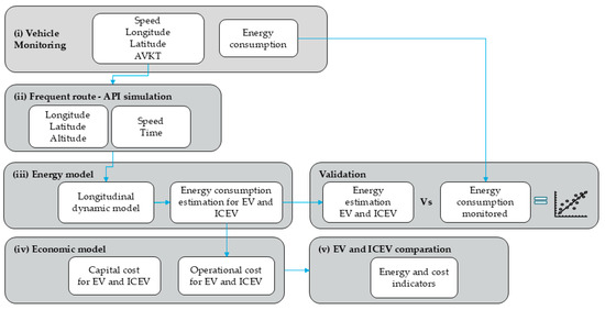
Figure 1.
Methodology used to estimate the energy consumption and operating costs of a fleet of electric and combustion vehicles.
- (i)
- Vehicle characterization and monitoring. The technical characteristics of the EVs used in the operation were identified. Monitoring equipment was installed in these vehicles to collect operating data. The data collected by the vehicles was used to determine the most frequent route, average travel speed and kilometers traveled.
- (ii)
- Route simulation with commercial applications. The google API and Open elevation provide longitude, latitude, and time required for the most frequent route. The data needed for predicting energy consumption is gathered by segmenting the route. In this way, it is possible to estimate consumption for routes that have not been monitored.
- (iii)
- Energy model construction. A longitudinal vehicle dynamics model is used to estimate vehicle energy consumption. The energy model is implemented to estimate vehicle consumption considering the route simulated by the Google API and the specifications of each vehicle. The model results include the measurement of technical performance indicators that allow comparing the operation with combustion vehicles of similar characteristics.
Model validation is carried out using speed, time, and altitude parameters obtained from vehicle monitoring as input variables. The model’s output is then compared against the consumption-related measurements recorded during the monitoring process. The model is subsequently refined to minimize the average error between estimated and observed energy consumption. A 5% error margin is established as the threshold for considering the model highly reliable.
- (iv)
- Economic model. The estimation of operating and capital costs—used to calculate the TCO—considers energy consumption, average annual kilometers traveled (AVKT), maintenance costs, and vehicle-specific characteristics.
- (v)
- Benchmarking. An energy and cost comparison is conducted to evaluate the implications of transitioning from ICEVs to EVs of similar characteristics.
2.1. Instrumentation and Vehicles Engaged
The vehicles under study provide transportation services for personnel and materials for the maintenance and repair of electrical networks in the city of Pereira, Colombia. Therefore, van and pickup vehicle types are used. Table 2 displays the technical characteristics of these vehicles [34,35].
Table 2.
Technical characteristics of vehicles considered in the study.
The vehicles were instrumented with equipment that connects to the CAN network and can acquire and store operating variables. The monitoring equipment provides signals such as engine RPM, speed, engine load and battery voltage. In addition, a GPS device collected position information (latitude and longitude). The vehicles were monitored for 2 months, following the company’s normal operation, which is from Monday to Saturday during daylight hours from 6 am to 5 pm. Occasionally the vehicles were used for repairs and overhauls on Sundays or holidays. The training of the drivers together with the constant review of the operation of the monitoring equipment made it possible to obtain a database with the energy consumption variables that were used to validate the results of the energy model.
2.2. Energy Consumption Model
In this study, a model based on longitudinal vehicle dynamics was used to estimate fuel consumption. The model implements the fundamental laws of physics to calculate the longitudinal external forces represented graphically in Figure 2.
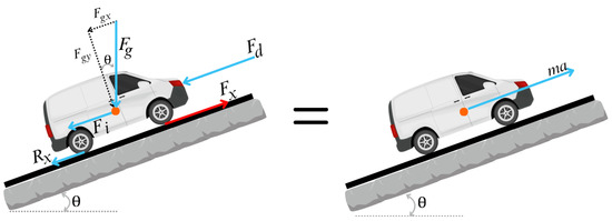
Figure 2.
Diagram of longitudinal forces present in vehicles [19].
The vehicle must overcome the forces opposing the movement. The required tractive force at the wheel can be calculated from Equation (1).
where is the traction force required by the vehicle to perform the motion, is the force caused by the aerodynamic drag, is the rolling resistance, is the longitudinal force caused by the weight of the vehicle considering the inclination and is the inertial force of the vehicle including the inertia of the rotational elements used in the vehicle transmission. The forces are calculated by means of Equations (2)–(5) [19].
where is the air density, is the frontal area of the vehicle, is the aerodynamic drag coefficient, is the vehicle speed, is the rolling coefficient, is the total vehicle mass, is the road camber angle, is the equivalent mass, which is composed of the total vehicle mass and the mass factor associated with the rotational components of the vehicle, and is the vehicle acceleration.
The frontal area of the tested vehicles was estimated through planimetric analysis of photographs. For the vehicle typology used in the analysis, the aerodynamic coefficient ranges between 0.5 and 0.7 [20]. The rolling coefficient depends on the tires of the vehicle and the road surface conditions. Table 3 shows the ranges of this coefficient for different scenarios [20].
Table 3.
Vehicle rolling coefficients according to road characteristics.
The vehicles included in the study are fitted with conventional tires and transit mainly over asphalt roads, so a coefficient of 0.02 was used [20]. The inertia force experienced by the vehicle in response to changes in speed is studied in terms of both translational and rotational kinetic energy. Inertia increases the vehicle’s effective mass due to the angular moment of rotating components. This equivalent mass is estimated using Equation (6), which considers a dynamic inertia factor [20].
where NTD is the final drive ratio of the vehicle; it is the result of the product of the differential ratio and the vehicle gear ratio in each gear. The EVs under study have automatic transmissions and feature a Continuously Variable Transmission (CVT). The power requirement is estimated by means of Equation (7).
where is the combined efficiency of the powertrain elements, which must be compensated to generate the required power.
There are conditions in which the resultant tractive force is negative. This is because the inertia force and the force due to the inclination gradient both contribute to the longitudinal motion of the vehicle. The instantaneous energy consumed by a vehicle engine can be estimated by Equation (8).
For the study, the energy consumed is determined in small segments with constant time intervals, where is equal to 1 s, so it must be converted to hours using the factor of 3600. The total energy consumed during a trip can be estimated as shown in Equation (9).
where represents the time, in seconds, that took the vehicle to complete the route. Currently, some vehicles feature a regenerative braking system that allows them to recover a portion of the energy. This system enables remnant kinetic energy from braking stages to be transformed into electricity, then used to charge the battery [20].
A direct correlation exists between traction power and the energy recovered through regenerative braking. When traction power is positive, it means that the vehicle’s tires receive energy from the propulsion system to generate vehicle motion, thus making the braking energy null. On the other hand, traction power is negative in braking stages, and a fraction of the energy is recovered to the battery [20]. Regenerative power is calculated through Equation (10).
where is the combined efficiency for energy regeneration, and is the regenerative braking factor. The combined efficiency is given by powertrain components and is one of the main differences between ICEVs and EVs.
For both ICEVs and EVs, the engine-to-tire transmission efficiency, as well as the engine’s efficiency, are taken into account. The electrical engine’s efficiency can be up to 95%, while the internal combustion engine does not go over 35% [36]. Figure 3 showcases an EV’s combined efficiency, which is given by Equation (11).
where is the transmission efficiency, is the mechanical efficiency of the engine, is the efficiency of the inverter, and is the battery discharge efficiency.
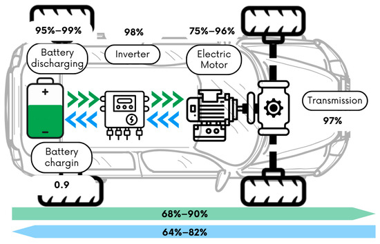
Figure 3.
EV powertrain and associated transmission efficiencies, where green represents energy consumption and blue energy regeneration.
When the electrical engine acts as a generator, a charging circuit converts electrical energy into chemical energy stored within the batteries. Taking the latter into consideration, the combined efficiency is modified as shown in Equation (12).
where is the battery’s charging efficiency.
The regenerative braking coefficient is related to the vehicle speed and can be estimated as shown in Equation (14) [19].
It is worth noting that when a vehicle’s deceleration exceeds 0.2 times gravity, the security system that maintains vehicle stability is activated. This system distributes energy throughout the conventional braking system, therefore preventing regeneration [36].
Regenerated energy from the vehicle’s braking system is calculated at one-second intervals, as shown in Equation (14).
Similarly, a vehicle’s total regenerated energy in its route is determined by Equation (15).
Taking into account the regenerated energy, total consumed energy can be represented through Equation (16).
where is the energy recovered through the vehicle’s braking system. This parameter becomes non-zero when the traction force () is negative, enabling energy recovery. The regenerated energy mathematically originates from and has an opposite sign to the tractive energy (), making the magnitude of equal to or less than . ICEVs do not have a regenerative braking system, thus making the recovered energy zero.
Monitoring data is used to validate the model. For that purpose, preliminary model results are obtained in short segments and compared with energy registered during monitoring. If the consumed and regenerated energy error margin surpasses 5%, efficiency and regeneration factor parameters are adjusted.
Various web applications are used to simulate a route, which includes strategic locations for the operation of the electric vehicle fleet. Google API allows the recreation of frequent routes by joining the operational hubs and segmenting the route according to changes in direction, stops, control points, and critical areas. This web application provides the distance and travel time for all segments. Each data point in the partition is georeferenced, allowing the integration with Open-Elevation API to obtain road altitude. Route speed and elevation are filtered and smoothed before being sent to the model as primary inputs. By using web applications to recreate a route, no monitoring is required, thus expanding the possible usages of the energy consumption model. Finally, after validating the model, energy consumption is evaluated on the frequent route to assess the transition from a fleet of 10 ICEVs to 5 vans and 5 electric pickups.
2.3. Economic Model
In this study, the Total Cost of Ownership (TCO) model is implemented, which incorporates governmental incentives, retailer discounts, and regulations that grant tax benefits such as a reduced Value-Added Tax, as well as a lower vehicle tax, from 3.5% to 1%, for EVs. To estimate and forecast costs, two scenarios are considered: the first scenario involves no battery replacement within a 10-year timeframe, and the second scenario includes the replacement occurring during the 8th operation year of a 15-year ownership horizon.
The TCO for the studied vehicles in a base year, 2024 in this case, is calculated through Equation (17) [12].
where CC is the cost of capital, and CO is the operating cost of the vehicles. The values used for every component are estimated based on the company’s information and secondary sources, such as government entities and car dealership websites [6,37]. The cost of capital is calculated through Equation (18).
where PV stands for the commercial price of the vehicle, and VR represents the resale value at the end of its lifetime. D denotes discounts offered by car dealerships, which may include exclusive offers or reductions for large purchases, while CM represents the registration cost of the vehicle [12]. Equation (19) is used to calculate the resale value.
where is the depreciation value, considered at 20% for EVs in this study, taking into account the accelerated depreciation as one of the incentives given by the Colombian government. This depreciation occurs within the first 5 years of vehicle ownership, and n is the analysis year [38]. For ICEVs, depreciation is constant at 7% until the end of the analysis timeframe [39]. The parameter n corresponds to the analysis year in which the vehicle is projected to be sold; therefore, the analysis year is equivalent to the vehicle sales year in this context. Meanwhile, represents the interest rate used to discount future cash flows to their present value. For this study, a 6.75% rate is considered, corresponding to the average Consumer Price Index (CPI) between 2020 and 2024 [40,41].
The operational cost is calculated with Equation (20).
where represents the vehicle maintenance and operation cost. In this case, 18% of the capital cost is assumed as the for ICEVs [38]. The EV maintenance cost is assumed to be 50% of the ICEV maintenance cost [40]. CS represents the cost of the Mandatory Traffic Accident Insurance (Seguro Obligatorio de Accidentes de Tránsito, or SOAT), including a 10% discount for EVs in accordance with Law 1964 of 2019 [6]. corresponds to the annual interest fee in the case of purchase financing, whether for an ICEV or an EV. represents the vehicular taxes that must be paid annually. refers to the cost of the energy used by the EV and the fuel consumed by ICEV on route. Equation (21) presents the latter, taking into account the vehicle kilometer traveled (VKT) and the predicted performance.
where stands for the average annual kilometers traveled by a vehicle, and is the fuel consumption [L/km] for ICEVs or energy consumption [kWh/km] for EVs. Finally, refers to the energy cost in [COP/kWh] for electrical energy and [COP/L] for fuel.
The last component from Equation (20) corresponds to the Net Present Value formula, with which operational costs are estimated for a period n of analysis, and COP is calculated for the base year, which in this case is 2024.
The input values used to estimate EVs and ICEVs capital and operational costs are presented in Table 4.
Table 4.
Inputs for capital and operating costs for vans and pickups in COP [6,42,43].
Once the costs of capital and operating costs are estimated, Equation (17) is used to calculate the TCO. However, this study is not limited to estimating the cost in the base year, but also analyzes the evolution of cost over 15 years, comparing the cost of EVs and ICEVs. The model also accounts for the depreciation of the vehicle over the holding period to assess the variance in the cost of capital.
The above is achieved by calculating the annual costs from 2024 to 2030. To estimate the cost of capital in each year (CPC), Equation (22), is used, where the estimated cost of capital in the base year is used and depreciated according to the percentage . In this way, the depreciation value of the vehicle during its useful life is discounted.
On the other hand, for calculating the operating costs (OPC) of the vehicle on a year-by-year basis over their useful lives, Equation (23) is used, where the value of the operation in the base year CO is taken and then discounted over time. This formulation provides a simplified financial adjustment using a one-period linear approximation to incorporate the time value of money. While based on conventional discounting practices, it represents a modeling choice that balances analytical simplicity with capturing the discount rate’s impact on operating costs.
Finally, the cost model serves to evaluate the transition of 10 ICEVs from the fleet to 5 electric vans and 5 electric pickups.
3. Results
The monitoring made it possible to identify the actual operating conditions of the electric vehicles in the company, which determined maximum speed, maximum acceleration, distance traveled, average percentage of battery charge, time stopped, and time in operation. Table 5, shows the characteristics of the monitored routes.
Table 5.
Operating characteristics of the monitored vehicles.
The operation of the monitored vehicles focuses on the urban areas of the cities of Pereira and Cartago, Colombia. Additionally, the following frequent locations are identified:
- (A) Main charging dock of electric vehicles.
- (B) Material warehouse.
- (C) Headquarters.
- (D) Electric vehicle charging station.
- (E) Branch office of the company in Cartago.
Figure 4 shows the route most frequently used by vehicles during the monitoring stage.
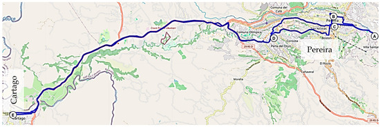
Figure 4.
Main route of operation (blue line) with frequent locations of the monitored electric vehicles.
The analysis of the monitoring data shows that the vehicles make frequent trips between the main charging dock (A) and the company’s materials warehouse (B). This route has a maximum measured slope of 25%. In Colombia, the maximum slope of roads ranges between 10 and 14% [44]. Therefore, this route is representative for the conditions of higher power demand for vehicles.
3.1. Validation of the Energy Consumption Model
A comparison is performed between the model estimate and the monitoring data for a van and a pickup vehicle. Tests were performed on short road segments with varying topography characteristics, while road segments with inadequate monitoring data were discarded during validation.
Preliminary findings indicated that the model underestimates the vehicle’s actual energy regeneration capacity. The relative error for all short trips averaged 25%, with an average determination coefficient of 0.73 for the trips analyzed. The error in the model estimation can be attributed to the values assumed for the study, such as the efficiency of the battery charging system and the estimation of the regenerative braking factor α as a function of speed. In this sense, a sensitivity analysis of the regenerative braking model was performed to adjust the factor proposed in Equation (14) considering the operating characteristics of the vehicles. The calculation of the adjusted regenerative brake factor is shown in Equation (24).
Table 6 shows the indicators estimated from the adjusted energy consumption model and the indicators estimated with the monitoring energy records for one of the trips. The results show that the model allows for the estimation of vehicle energy consumption with a total relative error of 2.1%. The estimation of energy consumed by traction presents an error of 2.08%, while regeneration shows an error of 1.97%.
Table 6.
Indicators for the evaluation of the operation of the vehicle fleet.
Figure 5 and Figure 6 show the comparison between the data measured during monitoring and the data estimated by the energy model. Figure 5 depicts a trip that begins at the main charging station (A) and ends at the material warehouse (B) at an average speed of 19 km/h. Figure 6 shows the consumption from the company’s headquarters (C) to the electric station (D). This route has a higher traffic density, with an average speed of 15 km/h, and peaks of up to 52 km/h. Panels a of Figure 5 and Figure 6 illustrate the energy consumed due to traction demand (), while panel d of each figure shows the energy regenerated along the route.
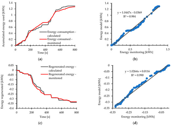
Figure 5.
Validation of energy model in comparison with monitoring—urban area and downtown; (a) validation of consumption, (b) energy consumption calculated and monitored, (c) validation of regeneration, (d) energy regeneration calculated and monitored.
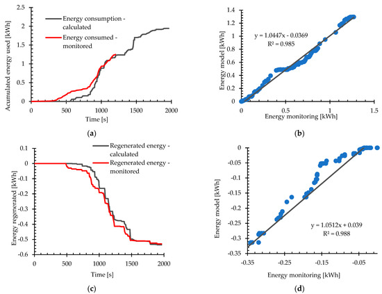
Figure 6.
Validation of energy model in comparison with monitoring—high traffic; (a) validation of consumption, (b) energy consumption calculated and monitored, (c) validation of regeneration, (d) energy regeneration calculated and monitored.
For all the routes studied in the validation, the average coefficient of determination was 95%, with the worst case being 92%. This indicates that the energy consumption model based on longitudinal vehicle dynamics can correctly estimate the energy demand on a route. Conversely, for the regenerated energy estimated with the model, the average coefficient of determination is 0.97.
Figure 7 shows the total energy consumption of a sample of nine route segments analyzed and validated against the monitored data of a van, providing an estimated MAPE of 7.6%. These segments exhibit variations in characteristics such as length, travel time, speed, and elevation changes, which resulted in an average consumption of 0.30 kWh/km. It was clear that topography has a significant influence on the final consumption of electric vehicles, given that a trip that started at 1400 m.a.s.l. (meters above sea level) and ended at 900 m.a.s.l. resulted in 0.19 kWh/km.
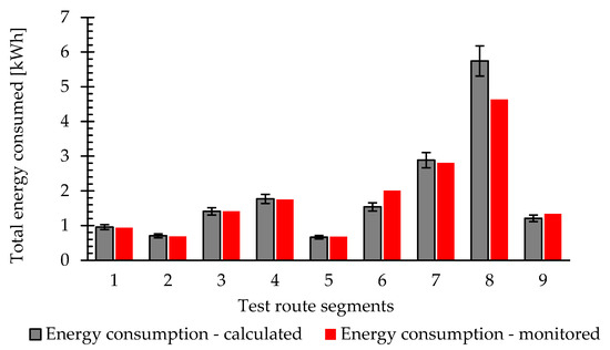
Figure 7.
Comparison of total energy consumption over various routes—van.
Power demand peaks are found in places where the road slope is the steepest. Figure 8 shows that the traction power required to complete the route is less than the maximum power of the monitored electric vehicle. Therefore, these EVs used to transport goods and people have the power needed to expand transit operations in other cities with similar characteristics to those evaluated.
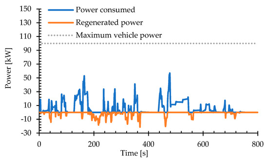
Figure 8.
Power demanded to make the trip.
To evaluate the model’s performance on an alternative vehicle type, monitoring data from a pickup was analyzed. Figure 9 shows the estimated and real energy consumed across seven route segment samples, achieving a 12.4% MAPE. The comparison between monitored and estimated energy yielded an average coefficient of determination of 0.91 for both consumption and regeneration. This study was not able to ensure that vehicles completed the same circuits as they continued their regular operation during monitoring. However, the energy consumption of the E-pickup was notably higher than that of the van, nearly doubling on a route with similar topography and driving behavior. While the van had an estimated consumption of 0.23 kWh/km, the pickup vehicle consumed 0.33 kWh/km.
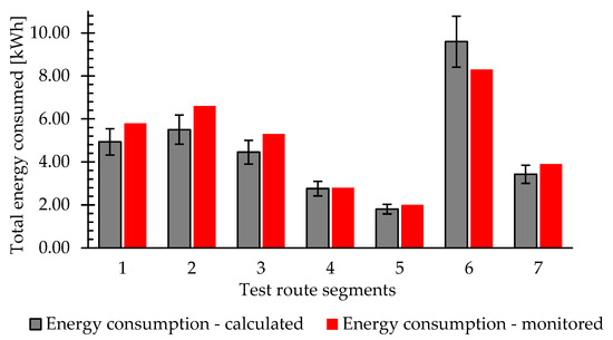
Figure 9.
Comparison of total energy consumption over various routes—pickup.
3.2. Estimated Energy Consumption for the Vehicle Fleet
The most frequent route was segmented and simulated through Google API to obtain the average altitude and speed required for estimating energy consumption using the model. The estimation was performed for the selected fleet, which includes electric and combustion vehicles, as well as van and pickup models. Figure 10 depicts the results of the analysis for each vehicle type, contrasting EV and ICEV performance.
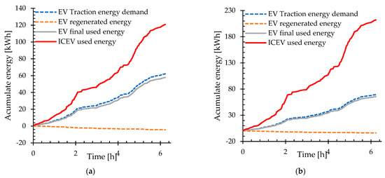
Figure 10.
Estimated energy consumption for (a) vans and (b) pickups.
The results reveal that the combustion van doubles its consumption compared to its electric counterpart, while the combustion pickup triples the energy consumption, even without taking regeneration into account. Additionally, given the characteristics of the route, it allowed an average regeneration of 4.3% of the energy used for traction, improving the performance of the EVs.
Regardless of the category, electric vehicles travel on average 2.1 km farther than combustion vehicles for each kilowatt of energy. In other words, electric vans and pickups can travel between 17.7 km and 20.9 km more than their combustion counterparts for each equivalent liter of gasoline. However, the useful range with the maximum charge available in the battery or tank reflects the varying energy storage capacities. The ICEV van has almost five times the range of the EV van, while the ICEV pickup has three times the range of the EV pickup. Table 7 summarizes all indicators derived from energy combustion on the frequent route.
Table 7.
Indicators of comparison between EV and ICEV on the most frequently used route.
Given the annual VKT of the vehicles analyzed, the fuel consumption of the ICEV fleet is estimated to be approximately 13 853 L of gasoline per year (4 883 L of gasoline for the vans and 8 966 L of gasoline for the pickups).
Energy usage is reduced by 62% by switching the fleet’s 10 ICEVs—5 vans and 5 pickups—to 5 EV pickups and 5 EV vans. In this change of technology, vans reduce their consumption by 53%, going from 45.6 MWh to 21.5 MWh per year. Similarly, energy usage is reduced by 70% with EV pickups, where consumption goes from 83.7 MWh to 24.7 MWh per year.
3.3. Cost Model Results
The analysis of operating costs is performed considering both the motorization technology and the vehicle type. These costs are estimated for the base year, i.e., the first year of the analysis period.
The yearly operating expenses per vehicle for a fleet consisting of five EV vans and five EV pickups are displayed in Table 8. Likewise, the annual cost of a fleet composed of ICEVs (five vans and five pickups) with similar characteristics is presented.
Table 8.
Comparison of operating costs.
The EV van has the lowest operating cost among the vehicles analyzed; when compared directly with the ICEV van, an 8.5% lower operating cost is identified. Likewise, when comparing the EV van with the EV pickup and ICEV pickup, the differences are 16.8% and 28.4%, respectively. This trend is maintained when analyzing the cost per kilometer traveled.
Among pickup vehicles, the electric vehicle has an operating cost of 13.8% lower compared to the combustion model. The results confirm that EVs represent a viable alternative in terms of operating costs. This is especially true when transitioning from light vehicles with high fuel consumption, such as pickup trucks, since the gap in operating costs is more pronounced.
Table 9 shows the TCO findings for the base year. From the results, it is evident that the TCO of EVs is approximately 10% higher than that of ICEVs. This discrepancy is due to the inclusion of acquisition costs. In particular, the commercial value of EVs is on average 41.45% higher than that of ICEVs, in addition to requiring charging infrastructure which contributes to the increased TCO.
Table 9.
Comparison of total cost of ownership.
The economic feasibility of battery replacement is evaluated by projecting the costs considering the defined scenarios. In scenario 1, the vehicle is operated for 10 years without replacing its battery, and in scenario 2, the battery is replaced in the 8th year of operation, maintaining the vehicle for 15 years. Figure 11 illustrates the results.
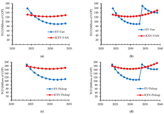
Figure 11.
TCO comparation for each type of vehicle both with and without considering battery replacement; (a) TCO comparation for van scenario 1, (b) TCO comparation for van scenario 2, (c) TCO comparation for pickup scenario 1, (d) TCO comparation for pickup scenario 2.
It can be inferred from Figure 11 that electric vehicles become cost-competitive after three years of operation for EV vans and from the second year of operation for EVpickups.
In the case of the EV van, the TCO begins in 2024 at a higher level than that of the ICEV van. From that point, it decreases steadily year by year. By 2026, the EV van already shows a lower TCO than the ICEV van, with an average difference of 28.10% in favor of the electric vehicle. This gap continues to widen as operational and maintenance (O&M) savings accumulate over time. By 2029, the cumulative savings in O&M costs reach COP 29.3 million, which exceeds the initial cost difference in COP 27.2 million between both technologies. From that year onwards, the initial cost overrun is fully amortized. The TCO then continues to decline slightly and stabilizes around 2032.
A similar behavior is observed for pickup vehicles. In 2024, the EV pickup starts with a higher TCO, but it also follows a downward trend. By the third year of operation—2026—the accumulated O&M savings amount to COP 30.5 million, which is approximately four times the initial cost difference. From that year onward, the TCO of the EV pickup remains consistently lower than that of the ICEV pickup, with an average reduction of 34.01%. The cost curve continues to flatten and stabilizes around 2031.
Furthermore, Figure 11 demonstrates that battery replacement has a large impact on the TCO of EVs, as there is a sharp increase in TCO in 2034, with increases of 87.2% for the EV van and 73.25% for the EV pickup, compared to the previous year. After battery replacement, although TCO decreases for both vehicles due to lower operating and maintenance costs, the economic impact for each vehicle type varies.
In the case of EV vans, the operational savings over their remaining lifetime do not offset the 40.6 million invested in the new battery, resulting in a cost overrun of 9.8 million compared to ICEV vans at the end of the analysis period. In contrast, for the EV pickups, the investment in the battery only increases the TCO by 9.3% compared to the ICEV pickups, representing a cost overrun of 17.8 million. Furthermore, at the end of the 15-year analysis, the cumulative operating savings of the EV pickups reach 32.3 million compared to the ICEV pickups, allowing the vehicle to operate longer, cover replacement costs, and maintain lower operating costs.
4. Discussion and Conclusions
This study developed and validated a methodology that enables the estimation of EV and ICEV energy consumption. By combining a longitudinal vehicle dynamics model with data from a web application, the methodology makes an important contribution to the analysis of vehicle fleets as it allows the estimation of consumption in different routes, without requiring the monitoring of vehicles. Additionally, the methodology allows the estimation of the TCO of a vehicle fleet, considering energy consumption, average annual vehicle travel, maintenance cost, and vehicle acquisition cost.
The energy consumption estimates exhibit a mean absolute percentage error (MAPE) of 7.6% when compared to actual vehicle monitoring data. In this sense, the energy consumption model developed allows the prediction of energy consumption with close approximations to reality. According to recent literature, state-of-the-art energy consumption models typically report relative errors of around 4.26% to 5.40%, depending on the estimation methodologies and the quality of the data employed [21,45]. In more challenging scenarios, relative errors can increase significantly, ranging from 12.4% to 33.9% [45]. The aforementioned studies implement machine learning techniques and real-time data feedback. Therefore, it can be inferred that the model implemented in this study presents an acceptable relative error for the estimation of vehicle energy consumption.
When evaluating the transition of a fleet of combustion vehicles composed of five vans and five pickups to five ICEV pickups and five ICEV vans for the operation of the company, comparative results of energy usage demonstrated that the company could reduce 62% of its energy consumption. Furthermore, the EV van’s and EV pickup’s respective ranges are 186 km and 215 km, which should be considered during route planning. This study not only evidences the energy viability and the benefits that the energy transition of a fleet of vehicles represents in urban pollution and the reduction in greenhouse gas emissions, but it also identifies the potential of the energy transition of business fleets and reduces the uncertainty of using this type of vehicles for the transportation of people and materials.
However, when directly comparing EVs to ICEVs, the former have lower operating costs. The EV van has an 8.5% lower operating cost than its combustion counterpart. Meanwhile, the operating cost of the EV pickup is 13.8% lower compared to the combustion model. However, for the base year, the TCO of EVs is about 10% higher than that of ICEVs. This is because the commercial value of electric vehicles is on average 41.45% higher than that of combustion vehicles, and they require a charging infrastructure. Even so, findings indicate that EVs start to become cost-competitive from the third year for EV vans and from the second year of operation for EV pickups.
The operational savings of the EV van during its remaining lifetime do not compensate for the investment in a new battery. In contrast, the investment in the battery only increases the EV pickup TCO by 9.3% compared to the ICEV pickup, which is fully depreciated due to the additional years of service. In this sense, the discussion centers on the fact that businesses that use E vans in their operation should have a strategy for auctioning the vehicle once the battery’s useful life is complete. The revenue from the sale could help offset the additional acquisition costs of the EV, allowing the company to anticipates greater financial gains from its second electric vehicle. The above confirms that EVs represent a viable alternative in terms of operating costs, particularly when transitioning from light vehicles with high fuel consumption such as pickup trucks, since the gap in operating costs is more pronounced.
The analysis identifies a vision of the electrification path that governments should follow to meet energy consumption and emissions targets. Companies with vehicle fleets may be more interested in energy transition if policies and regulations provide greater economic benefits., particularly for the cost of capital since there is still a significant difference in the acquisition prices of EVs compared to ICEVs. In addition, corporate EV fleets could be powered from their own charging stations, which reduces the uncertainty of available charging infrastructure in cities or road corridors. Also, it is identified that policies should focus on implementing strategies such as
- -
- Establishing an organization that supports technical and economic feasibility analyses for companies transitioning to EVs with vehicle fleets.
- -
- Creating an education plan on vehicle electrification at the business level, as the cultural landscape in Latin America warrants it.
- -
- Continuing the implementation of protected urban air zones, as this increases the motivation for the acquisition of this type of vehicles.
This study enables us to assess the energy and economic benefits of switching to electric vehicle fleets, even though it identifies possible limitations that should be taken into account in future studies. Initially, the methodology is validated for light-duty vehicles, and it is necessary to address other vehicle categories. Additionally, the methodology does not consider the impact of temperature on the energy consumption of electric vehicles. This factor can affect the performance indicators of the fleet. Similarly, an analysis of charging logistics for vehicle fleets is not yet included. Incorporating these parameters into analysis could enhance the fleet’s energy and economic metrics. In the Latin American context, it is crucial to assess the transition of freight fleets and motorbikes. The latter implies an additional challenge in terms of monitoring and standardization of operating parameters. Conversely, even if the study shows that owning EVs is economically feasible, for fleets of cars that provide public transportation services, such as cabs and rentals, a financial analysis is still necessary. The above serves to both establish if service rates are competitive with those of combustion vehicles, as well as to determine the specific incentives to be granted by governments. Finally, this study does not consider the charging times of the analyzed vehicles, a factor that may pose an operational barrier and increase maintenance costs due to the higher energy consumption associated with prolonged charging periods [3]. Therefore, future research could expand the characterization of vehicles to identify those with lower energy consumption based on optimized charging times.
Author Contributions
J.C.C.: Investigation, Formal analysis, Writing—review and editing, Methodology, and Funding acquisition; M.C.: Investigation, Formal analysis, and Writing—original draft; M.I.: Investigation, Formal analysis, and Writing—original draft; A.F.U.: Investigation, Writing—review and editing, and Funding acquisition; J.E.T.: Conceptualization, Methodology, Supervision, and Formal analysis; M.G.: Validation and Writing—review and editing; A.R.: Validation and Writing—review and editing; C.C.R.: Investigation and Writing—review and editing. All authors have read and agreed to the published version of the manuscript.
Funding
The research “Digital tool for the analysis of the operation, logistics and maintenance of the fleet of electric vehicles of the Energy Company of Pereira”, identified with code 6911-913-94153, which has led to these results, has received funding from the Ministry of Science, Technology and Innovation (Minciencias) under Grant 913—tax benefits for investment in science, technology and innovation projects year 2022.
Data Availability Statement
The original contributions presented in this study are included in the article. Further inquiries can be directed at the corresponding author.
Acknowledgments
The authors acknowledge the Energy Management research group (GENERGÉTICA), the Technological University of Pereira and the EAFIT University for their contribution to the development of this research, as well as the Empresa de Energía de Pereira (EEP) for data and technical collaboration.
Conflicts of Interest
The authors declare no conflicts of interest.
Abbreviations
| EV | Electric Vehicle |
| VKT | Vehicle Kilometers Traveled |
| MAPE | Mean Absolute Percentage Error |
| TCO | Total Cost Ownership |
| CC | Capital Cost |
| ICEV | Internal Combustion Engine Vehicle |
| LHV | Lower Heating Value |
| AVKT | Average Vehicle Kilometers Traveled |
| API | Application Programming Interface |
| CO | Cost of Operations |
References
- Andrade, N.F.; de Lima Junior, F.B.; Soliani, R.D.; de Souza Oliveira, P.R.; de Oliveira, D.A.; Siqueira, R.M.; da Silva Nora, L.A.R.; de Macêdo, J.J.S. Urban mobility: A review of challenges and innovations for sustainable transportation in Brazil. Rev. Gest. Soc. E Ambient. 2023, 17, e03303. [Google Scholar] [CrossRef]
- Correa, C.; Di Chiara, L. Banco Interamericano de Desarrollo (BID). Beneficios de la Electrificación: Estudio del Caso del Transporte Colectivo eléctrico en Uruguay. 2020. Available online: http://www.iadb.org (accessed on 12 May 2025).
- Agency, I.E. Global EV Outlook 2024 Moving Towards Increased Affordability. 2024. Available online: http://www.iea.org (accessed on 10 February 2025).
- Ministerio de Energía de Chile. Estrategia Nacional De Electromovilidad; Ministerio de Energía de Chile: Santiago, Chile, 2021. [Google Scholar]
- Dirección de Políticas de Mitigación al Cambio Climático and Gobierno de México. Estrategia Nacional de Movilidad Eléctrica. 2023. Available online: https://www.gob.mx/cms/uploads/attachment/file/832517/2.3.ENME.pdf (accessed on 12 May 2025).
- Congreso de Colombia. Ley 1964. 2019. Available online: https://www.minambiente.gov.co/documento-entidad/ley-1964-de-2019/ (accessed on 10 February 2025).
- Banco Interamericano de Desarrollo (BID). Impacto Económico De La Transición Energética En Perú. 2024. Available online: http://www.iadb.org (accessed on 12 May 2025).
- Ebie, E.; Ewumi, O. Electric vehicle viability: Evaluated for a Canadian subarctic region company. Int. J. Environ. Sci. Technol. 2021, 19, 2573–2582. [Google Scholar] [CrossRef]
- Lei, X.; Zhong, J.; Chen, Y.; Shao, Z.; Jian, L. Grid Integration of Electric Vehicles within Electricity and Carbon Markets: A Comprehensive Overview. eTransportation 2025, 25, 100435. [Google Scholar] [CrossRef]
- Li, Z.; Chen, Z.; Li, H.; Guan, C.H.; Zhong, M. On the value of orderly electric vehicle charging in carbon emission reduction. Transp. Res. D Transp. Environ. 2024, 135, 104383. [Google Scholar] [CrossRef]
- Briceno-Garmendia, C.; Qiao, W.; Foster, V. The Economics of Electric Vehicles for Passenger Transportation; World Bank Publications: Washington, DC, USA, 2023. [Google Scholar]
- Suttakul, P.; Wongsapai, W.; Fongsamootr, T.; Mona, Y.; Poolsawat, K. Total cost of ownership of internal combustion engine and electric vehicles: A real-world comparison for the case of Thailand. Energy Rep. 2022, 8, 545–553. [Google Scholar] [CrossRef]
- Günther, H.O.; Kannegiesser, M.; Autenrieb, N. The role of electric vehicles for supply chain sustainability in the automotive industry. J. Clean. Prod. 2015, 90, 220–233. [Google Scholar] [CrossRef]
- Yuksel, T.; Michalek, J.J. Effects of regional temperature on electric vehicle efficiency, range, and emissions in the united states. Environ. Sci Technol. 2015, 49, 3974–3980. [Google Scholar] [CrossRef]
- Burra, L.T.; Sommer, S.; Vance, C. Free-ridership in subsidies for company- and private electric vehicles. Energy Econ. 2024, 131, 107333. [Google Scholar] [CrossRef]
- Lebeau, K.; Lebeau, P.; Macharis, C.; Van Mierlo, J. How expensive are electric vehicles? A total cost of ownership analysis. World Electr. Veh. J. 2013, 6, 996–1007. [Google Scholar] [CrossRef]
- Figenbaum, E. Retrospective Total cost of ownership analysis of battery electric vehicles in Norway. Transp. Res. D Transp. Env. 2022, 105, 103246. [Google Scholar] [CrossRef]
- Durkin, K.; Khanafer, A.; Liseau, P.; Stjernström-Eriksson, A.; Svahn, A.; Tobiasson, L.; Andrade, T.S.; Ehnberg, J. Hydrogen-Powered Vehicles: Comparing the Powertrain Efficiency and Sustainability of Fuel Cell versus Internal Combustion Engine Cars. Energy 2024, 17, 1085. [Google Scholar] [CrossRef]
- Zhang, X.; Zhang, Z.; Liu, Y.; Xu, Z.; Qu, X. A review of machine learning approaches for electric vehicle energy consumption modelling in urban transportation. Renew Energy 2024, 234, 121243. [Google Scholar] [CrossRef]
- Ehsani, M.; Gao, Y.; Longo, S.; Ebrahimi, K.M. Modern Electric, Hybrid Electric, and Fuel Cell Vehicles, 3rd ed.; CRC Press: Boca Raton, FL, USA, 2018. [Google Scholar]
- Feng, Z.; Zhang, J.; Jiang, H.; Yao, X.; Qian, Y.; Zhang, H. Energy consumption prediction strategy for electric vehicle based on LSTM-transformer framework. Energy 2024, 302, 131780. [Google Scholar] [CrossRef]
- Yılmaz, H.; Yagmahan, B. Electric vehicle energy consumption prediction for unknown route types using deep neural networks by combining static and dynamic data. Appl. Soft Comput. 2024, 167, 112336. [Google Scholar] [CrossRef]
- Bolovinou, A.; Bakas, I.; Amditis, A.; Mastrandrea, F.; Vinciotti, W. Online prediction of an electric vehicle remaining range based on regression analysis. In Proceedings of the 2014 IEEE International Electric Vehicle Conference (IEVC), Florence, Italy, 17–19 December 2014; pp. 1–8. [Google Scholar] [CrossRef]
- Miri, I.; Fotouhi, A.; Ewin, N. Electric vehicle energy consumption modelling and estimation—A case study. Int. J. Energy Res. 2021, 45, 501–520. [Google Scholar] [CrossRef]
- Zhao, X.; Ye, Y.; Ma, J.; Shi, P.; Chen, H. Construction of electric vehicle driving cycle for studying electric vehicle energy consumption and equivalent emissions. Environ. Sci. Pollut. Res. 2020, 27, 37395–37409. [Google Scholar] [CrossRef]
- Modi, S.; Bhattacharya, J.; Basak, P. Estimation of energy consumption of electric vehicles using Deep Convolutional Neural Network to reduce driver’s range anxiety. ISA Trans. 2020, 98, 454–470. [Google Scholar] [CrossRef]
- Wang, Z.; Liu, Z.; Cheng, Q.; Gu, Z. Integrated self-consistent macro-micro traffic flow modeling and calibration framework based on trajectory data. Transp. Res. Part C Emerg. Technol. 2024, 158, 104439. [Google Scholar] [CrossRef]
- Chen, Y.; Wu, G.; Sun, R.; Dubey, A.; Laszka, A.; Pugliese, P. A Review and Outlook of Energy Consumption Estimation Models for Electric Vehicles. arXiv 2020, arXiv:2003.12873. [Google Scholar]
- Zhang, J.; Wang, Z.; Liu, P.; Zhang, Z. Energy consumption analysis and prediction of electric vehicles based on real-world driving data. Appl. Energy 2020, 275, 115408. [Google Scholar] [CrossRef]
- Chakraborty, A.; Lopez, G.; Beatriz, J. Assessing the Total Cost of Ownership of Electric Vehicles Among California Households; UC Office of the President: Oakland, CA, USA, 2024. [Google Scholar] [CrossRef]
- Gahlaut, T.; Dwivedi, G. A Comprehensive Study for Multi-Criteria Comparison of EV, ICEV, and HEV. arXiv 2024. [Google Scholar] [CrossRef]
- See, C.Y.; Santos, V.R.; Woodley, L.; Yeo, M.; Palmer, D.; Zhang, S. Prices and preferences in the electric vehicle market. arXiv 2024, arXiv:2403.00458. [Google Scholar]
- Mauritzen, J. With great power (prices) comes great tail pipe emissions? \\ A natural experiment of electricity prices and electric car adoption. arXiv 2023. [Google Scholar] [CrossRef]
- BYD. BYD T3. 2022. Available online: http://www.bydauto.com.co (accessed on 13 June 2025).
- JAC. Ficha Técnica Jac T8. 2022. Available online: https://www.jac.cr/jac/site/docs/20230317/20230317205314/ficha_tecnica_t8_ev.pdf (accessed on 13 June 2025).
- Asamer, J.; Graser, A.; Heilmann, B.; Ruthmair, M. Sensitivity analysis for energy demand estimation of electric vehicles. Transp. Res. D Transp. Environ. 2016, 46, 182–199. [Google Scholar] [CrossRef]
- Ya, C. Carros Eléctricos: Incentivos y Descuentos por su Compra en Colombia. Available online: https://www.carroya.com/noticias/guias-de-compra-y-venta/carros-electricos-incentivos-y-descuentos-por-su-compra-en-colombia (accessed on 13 May 2025).
- Ministerio de Ambiente y Desarrollo Sostenible. Deducción por Depreciación Acelerada en Inversiones en Fuentes no Convencionales de Energía FNCE. 2020. Available online: https://beneficios-tributarios.minambiente.gov.co/incentivo-contable-deduccion-por-depreciacion-acelerada-de-equipos-y-obras-civiles-destinados-a-proyectos-de-fnce/ (accessed on 6 June 2025).
- FASECOLDA. Guía de Valores; FASECOLDA: Bogotá, Colombia, 2025. [Google Scholar]
- Cuéllar-Álvarez, Y.; Clappier, A.; Rojas-Roa, N.Y.; Thunis, P.; Mangones, S.; Belalcázar-Cerón, L.C. Emissions and ownership-cost of conventional and electric passenger vehicles in Bogotá, Colombia. Transp. Res. D Transp. Env. 2024, 128, 104105. [Google Scholar] [CrossRef]
- Departamento Administrativo Nacional de Estadística (DANE). Índice de Precios al Consumidor -IPC Histórico. Available online: https://www.dane.gov.co/index.php/estadisticas-por-tema/precios-y-costos/indice-de-precios-al-consumidor-ipc/ipc-historico (accessed on 13 May 2025).
- Secretaría de Movilidad Distrital. Matrícula de Vehículos Automotores Ventanilla Única de Servicios. Available online: https://www.ventanillamovilidad.com.co/tramites/matricula (accessed on 4 May 2025).
- BBVA. Simula tu Crédito de Vehículo. Available online: https://www.bbva.com.co/personas/productos/prestamos/vehiculo/herramientas/simulador/?cid=sem::gsa:00015746-vehiculo_gnral_aon_sem_gsa_text_cpc_web_ds_acn_b-pre-leasing_de_vehiculo:om_om_gen_mxcli_v1-perf-tff:::bbva%20credito%20vehicular:b:::text:dinamico::&gad_source=1&gclid=Cj0KCQiAwtu9BhC8ARIsAI9JHal-NiYT42Wni9jqmpSmfp2EIEX5R1CE1SuzrEXC_sMcbDPfn7Yai1QaAmuAEALw_wcB&gclsrc=aw.ds (accessed on 4 May 2025).
- Ministerio de Transporte de Colombia. Manual de Diseño Geométrico de Carreteras; Ministerio de Transporte de Colombia: Bogotá, Colombia, 2008. [Google Scholar]
- Jiang, Y.; Guo, J.; Zhao, D.; Li, Y. Intelligent energy consumption prediction for battery electric vehicles: A hybrid approach integrating driving behavior and environmental factors. Energy 2024, 308, 132774. [Google Scholar] [CrossRef]


Disclaimer/Publisher’s Note: The statements, opinions and data contained in all publications are solely those of the individual author(s) and contributor(s) and not of MDPI and/or the editor(s). MDPI and/or the editor(s) disclaim responsibility for any injury to people or property resulting from any ideas, methods, instructions or products referred to in the content. |
© 2025 by the authors. Licensee MDPI, Basel, Switzerland. This article is an open access article distributed under the terms and conditions of the Creative Commons Attribution (CC BY) license (https://creativecommons.org/licenses/by/4.0/).