Abstract
Northeastern Brazil (NEB) has a high potential for wind energy generation, making it a strategic area for the development of this renewable source. However, the region’s complex wind regime, driven by interactions between large-scale atmospheric systems, local circulations, and coastal topography, presents significant challenges for weather forecasting and wind energy applications. Despite this, detailed assessments of forecast performance using mesoscale models remain limited. The main objective was to develop an efficient strategy that enables satisfactory results by optimizing data assimilation, land use and topography information as well as improvements in physical parameterizations and post-processing, optimizing computational effort. Forecasting conducted during the year 2020 were validated with data from 20 anemometric measurement towers (AMTs), located at strategic points across various wind power complexes. The model’s performance was evaluated using statistical metrics such as MBE, MAE, nRMSE, standard deviation ratio, and correlation. Additionally, the impact of bias removal was assessed using two approaches: one that eliminates the mean error per forecasted time step and another employing artificial intelligence for bias removal training. The results revealed distinct characteristics for each analyzed location, with errors of diverse nature due to the local nuances of the measurements. However, both bias removal approaches showed significant improvements in wind characterization across all complexes.
1. Introduction
Most wind farms in Brazil are concentrated in the Northeast [1,2] a tropical region of strategic importance to the national energy mix, an importance projected to persist even under future climate scenarios [3,4,5,6,7,8]. Despite advances in short-term forecasting, model performance remains limited in the region due to high heat and moisture, which intensify convective systems and trigger extreme rainfall and wind gusts [9,10,11,12,13]. Its complex wind patterns arise from interactions among large-scale atmospheric systems such as southeast trade winds influenced by the Intertropical Convergence Zone (ITCZ), the South Atlantic Subtropical High (SASH), easterly wave disturbances (EWDs) and local land–sea breezes, combined with mesoscale dynamics shaped by topography and coastal contrasts [14,15]. Surface heterogeneities, including elevation gradients, variable vegetation, and land use patterns, further intensify turbulence and impact boundary layer development [16,17,18,19], posing challenges for high-resolution wind modeling essential to renewable energy forecasting.
Numerical weather prediction models simulate atmospheric behavior using physics and thermodynamics equations to represent radiative, chemical, physical, and dynamic processes [20,21,22,23,24]. Although parametrization schemes have advanced for tropical regions like Brazil [9,11,12,25,26,27,28], accurately resolving the planetary boundary layer (PBL) remains a major challenge. The PBL patterns, driven by turbulent vertical transport of mass, heat, and moisture, are highly sensitive and difficult to capture in models [29,30,31,32,33,34,35], but its internal processes have a direct impact on wind forecast accuracy, especially for wind energy applications [36,37,38,39,40,41].
Despite the Northeast region’s strategic role in Brazil’s renewable energy sector, relatively few studies have applied high-resolution atmospheric models to assess its wind conditions. Given the high spatiotemporal variability of wind speed, which causes power production fluctuations and demands predictive accuracy, precise short- and long-term forecasts are critical for grid operators [36]. The Weather Research and Forecasting (WRF) model, developed through collaborations among U.S. government agencies and a broad scientific community, is widely used for wind energy forecasting due to its flexible physics and dynamic configurations suited for both research and operational use [42,43,44,45]. WRF has proven effective in simulating near-surface winds when enhanced through data assimilation, customized parametrizations, and bias correction, but its operational use in NEB remains limited, with few efforts focused on calibrating its physical schemes, terrain data, and land cover inputs [46,47]. Enhancing wind forecast accuracy is essential to optimize energy dispatch, anticipate ramp events, and support maintenance and grid integration strategies.
This study assessed the cost-effective configuration for the potential of the WRF mesoscale model to operational forecast wind variability in the Northeast Brazil (NEB), a region critical for wind energy, with the cost–benefit for applications without reliance on high-cost infrastructure. Forecasting was conducted at synoptic hours (00:00, 06:00, 12:00, and 18:00 UTC) using the Global Forecast System (GFS) as input (~28 km resolution) and included updated topographic (SRTM), land-use (MapBiomas) data, optimized physical parameterizations, spectral nudging as data assimilation, and bias-correction methods to address uncertainties from subgrid-scale process approximations [48,49,50]. Model outputs were validated against data from 20 atmospheric meteorological towers (AMTs) throughout 2020, each AMT belonging to a different wind farm; however, station locations were omitted due to confidentiality agreements. The results demonstrate that this accessible, low-cost configuration framework can effectively support wind farm operations and maintenance while offering a practical foundation for improving local forecasts through future enhancements such as statistical downscaling.
2. Materials and Methods
2.1. CER-UFPE Wind Power Forecasting Tool
The WRF configured and used in this study is part of a broader forecasting framework originally developed under the High-Performance Computing for Energy (HPC4E) project. This methodology is based on the combination of predictive models of different natures (Figure 1), and is hereafter referred to as the CER-UFPE wind power forecasting tool.
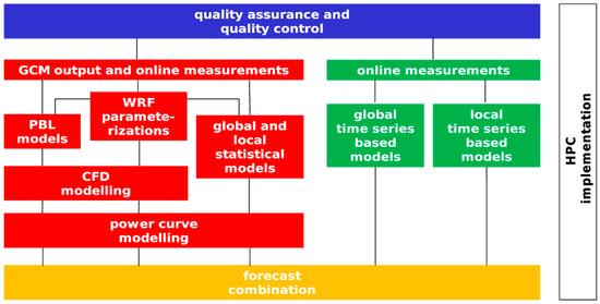
Figure 1.
Descriptive flowchart of the CER-UFPE wind power forecasting tool. Source: The authors.
The tool was designed to ingest new data through a file repository, with a connector responsible for continuously monitoring and integrating observational data provided by the wind farm operator (e.g., supervisory control and data acquisition—SCADA systems and anemometric measurement towers—AMTs). In addition, the tool directly acquires data from external sources via the Internet such as operational numerical forecast fields from official repositories (e.g., the Global Forecast System—GFS).
Conceptually, the general framework of the CER-UFPE wind power forecasting tool is illustrated in Figure 1, which depicts its three modes of operation: (a) calibration mode—training the models using historical datasets to infer parameters prior to operational deployment; (b) Operation mode—generation of real-time or near-real-time forecasts at multiple time scales (hourly, daily, and monthly); (c) Recalibration mode—periodic retraining of selected models to mitigate forecast drifts and ensure long-term reliability.
These models utilize observational data of wind speed, wind direction, and active power from wind farms, both for training and operational forecasting. The quality of the input data was rigorously assessed using a combination of global and local statistical tests, with a particular focus on identifying and removing outliers that could compromise forecast accuracy [51]. The framework also integrates mesoscale atmospheric modeling (based on WRF) and microscale modeling (based on OpenFOAM), advanced statistical downscaling and machine learning techniques for local wind conditions, refined power curve modeling to convert wind forecasts into power forecasts, linear and nonlinear time series models with online learning capabilities, and ensemble forecasting approaches.
The forecasting framework integrates six main types of models, which together provide wind speed and active power predictions at hourly, daily, and monthly scales. On the hourly scale, forecasts extend up to 7 days ahead, with 30 min time steps and particular emphasis on the first 48 h. For the daily scale, the forecasts have a 1-day resolution and a maximum horizon of 15 days. For the monthly scale, the forecasts are produced with 1-month time steps and extend up to 3 months ahead. This multi-scale design enables the tool to support forecasting solutions ranging from short-term operational needs to longer-term (seasonal) planning.
The application of the WRF model in this study was restricted to hourly scale forecasts. Forecast releases (model cycles) followed the GFS, which was updated four times per day (00, 06, 12, and 18 UTC). The outputs from each WRF run were subsequently used to provide hourly wind speed forecasts that serve as the input for the statistical downscaling models, power curve modeling, and computational fluid dynamics (PBL and CFD) simulations.
Nevertheless, the computational demand of employing WRF as a provider of the initial and boundary conditions for other models can be a limiting factor, given the time required to perform dynamic downscaling. To address this, the methodology of the present study was structured into three main stages, each targeting a critical component of forecast optimization. To ensure accurate mesoscale forecasts for the Northeast Brazilian region (NEB), the following strategy was adopted: (a) High-resolution geographic data integration—incorporation of updated land-use and topographic datasets to refine surface representation; (b) Optimized physical parameterizations—selection of schemes designed to improve the simulation of atmosphere–surface interactions; (c) Data assimilation through spectral nudging—applied to enhance the initialization of atmospheric fields and maintain coherence with large-scale circulation patterns. To ensure computational performance, a domain with a 9 km resolution was used in an optimized domain with 61 vertical levels, improving model performance while maintaining accuracy.
Performance was the central criterion across all stages, aiming to balance accuracy with computational efficiency. These steps were designed to enhance the realism, reliability, and spatial consistency of deterministic forecasts, particularly for the set of AMTs managed by the private company.
2.2. Infrastructure
The computational experiments in this study were performed on a server equipped with a 64-bit x86_64 architecture (Little Endian), supporting both 32-bit and 64-bit operations. The system was powered by two AMD EPYC 7413 24-Core (Dell, Round Rock, TX, USA) processors, yielding a total of 48 physical cores with no simultaneous multi-threading (1 thread per core). The processor architecture was organized into two physical sockets, distributed across eight NUMA (non-uniform memory access) nodes, each comprising six dedicated cores. This NUMA segmentation improves memory management and parallel task execution by reducing latency and enhancing data locality. Each core operates at a base clock speed of approximately 1.5 GHz. The system provides a multi-level cache architecture including 64 MB of shared L3 cache across all cores. This configuration ensures computational efficiency for parallel scientific modeling.
To optimize model performance, the WRF Registry was customized to output only essential variables. This reduced the I/O time and storage requirements, improving the simulation efficiency. Moreover, this configuration optimized post-processing by reducing disk storage demand and I/O time, enabling the retention of larger forecast archives. The selected variables in this study were defined to ensure the full functionality of the CER-UFPE wind power forecasting tool.
2.3. Observational Dataset
The wind data from the AMTs used in this study are proprietary and protected by confidentiality agreements; therefore, the names of the wind farms and their complexes have been omitted, and the sites were instead anonymized as T1 to T20. For subsequent discussion, the towers were consolidated into four complexes—C1, C2, C3, and C4—each covering a specific set of AMTs (Figure 2). All raw time-series retrieved from the anemometers and wind vanes were subjected to the dedicated quality-control module [51], embedded in the CER-UFPE wind power forecasting tool prior to use.
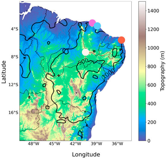
Figure 2.
Topography (m) of Northeast Brazil, represented by the color gradient, derived from SRTM data. Black contour lines indicate GPCC precipitation climatology (mm) over the region. The locations of the 20 anemometric measurement towers (AMTs), used for model validation, were overlaid as point markers, C1 (light blue), C2 (purple), C3 (light gray), and C4 (red). Precipitation climatology over the NEB was obtained from the Global Precipitation Climatology Center (GPCC) database (https://psl.noaa.gov/, accessed on 16 December 2024).
Data from 20 AMTs managed by a private company were used, providing wind speed and direction measurements at 90 m and 100 m heights across different parts of Northeast Brazil. The towers are in diverse settings, some near the coast, while others are inland, each influenced by distinct topographic and atmospheric conditions. The region’s climate is highly complex, with wind farms subject to varying rainfall and wind regimes shaped by large-scale atmospheric systems, local topography, and coastal–inland contrasts. These combined factors result in significant spatial variability in wind and precipitation over relatively short distances.
2.4. Geographic Dataset
The wind profile is significantly influenced by land surface roughness and vegetation canopy height [52,53,54]. Land use and cover, sourced from the MapBiomas platform, were incorporated to enhance the solutions for surface heat and moisture fluxes simulated by the WRF model [47]. MapBiomas data, freely available with 90 m resolution, are updated annually and provide information on various surface classes like water bodies, forests, and grass. Topographic data, also critical for roughness, were incorporated from the Shuttle Radar Topography Mission (SRTM) version 4, with 90 m resolution. These data were incorporated into the WRF pre-processing system (WPS) prior to any validation or operational simulation.
Northeastern Brazil exhibits a highly complex diversity of climate, topography, and vegetation. As illustrated in Figure 2, the region’s rugged terrain imposes spatial particularities that directly influence rainfall regimes, which vary according to the location of each distributed wind farm complex. For instance, Complex C4 is situated within the rainfall regime of the eastern coastal region, characterized by a rainy season from April to August and an annual precipitation exceeding 1200 mm and a height above sea level of nearly 70 m. In contrast, Complex C3 lies in a semiarid climate zone, with an annual rainfall around 600 mm, concentrated between January and April and a height above sea level of more than 1000 m. Complexes C1 and C2, on the other hand, experience over 1000 mm of precipitation annually, also with a rainy season concentrated in the first four months of the year, at sea level and near the coastline. It is important to note that the meteorological phenomena responsible for rainfall vary among the complexes. While Complex C4 is mainly influenced by easterly wave disturbances (EWDs), Complexes C1, C2, and C3 are predominantly affected by the Intertropical Convergence Zone (ITCZ).
Beyond climatic factors, topography also plays a role in the spatial arrangement of the wind complexes, presenting nuances relevant to analysis. Table 1 shows the estimated distance of each complex from the coastline, a factor that can directly impact wind conditions and the operational efficiency of wind forecasting.

Table 1.
Wind power complex and the estimated distance from the coastline.
2.5. Physical Parameterization
The WRF model uses interconnected physical modules to simulate key atmospheric processes, with flexible parameterization schemes tailored to research needs. The cumulus cloud physics module simulates convective processes and precipitation, while the cloud microphysics module handles smaller-scale processes like condensation and evaporation. Radiation is modeled through shortwave and longwave schemes that calculate atmospheric heating and energy balance. The planetary boundary layer (PBL) module manages turbulent mixing, linking subgrid-scale processes with larger dynamics. The surface-layer physics module computes heat and moisture fluxes, which are integrated with soil properties to model land–atmosphere interactions. These modules work together to simulate the atmosphere’s evolution with physical realism, enabling accurate mesoscale forecasting. The WRF model, widely used in the scientific community, is periodically updated, with version 4.4 employed in this study with specific parameter combinations.
Defining an appropriate set of parameterizations for a given site requires a computationally intensive sensitivity analysis, since the large number of possible parameter combinations demands that each candidate configuration be individually simulated and validated, as demonstrated in several sensitivity studies [11,12,55,56,57,58,59]. To reduce this cost, we used an efficient sampling strategy. First, we identified the period with the most significant meteorological activity (instabilities) across the measurement towers. Then, within that period, we selected the tower with the highest hourly variability, assuming that it was the most difficult to represent numerically. After choosing the parameter combinations that yielded the best performance for the AMT during the unstable period, we ran forecasts for the most stable period to confirm the robustness of the results in both periods. The parameter set showing the most consistent performance for the region of interest is summarized in Table 2.
Table 2.
Parameterizations used in the WRF model after sensitivity analysis.
Finally, we deployed this parameter suite in the production runs and benchmarked the results against observations from every remaining AMT, confirming the configuration’s overall robustness. After conducting accuracy and performance tests to identify a representative domain, we verified that the configuration of 170 × 170 grid points, with a horizontal resolution of 9 km and 61 vertical levels following the topography, provided the best optimization for the region. This domain presented satisfactory results, balancing the simulation time with the ability to resolve mesoscale meteorological phenomena. It is worth noting that the CER-UFPE wind power forecasting tool already offers statistical downscaling and short-term nowcasting modules to refine near-surface fields, so our effort focused on selecting the optimum physical parameterization set that maximized forecast accuracy while minimizing the computational expense.
2.6. Data Assimilation and Forecast Runs
Spectral nudging was employed as an indirect data assimilation technique to maintain consistency between the regional model and large-scale atmospheric fields. Unlike grid nudging, which strongly constrains small-scale variability, spectral nudging only acts on wavelengths above a defined cutoff, relaxing selected atmospheric variables (horizontal wind, potential temperature, and geopotential) toward the driving global model through spectral decomposition [67,68]. This approach allows large-scale circulations to be more accurately represented while mesoscale processes develop freely within the domain [69,70,71,72]. In this study, the WRF model was configured with four-dimensional data assimilation (FDDA) using spectral nudging, incorporating large-scale atmospheric fields from the Global Forecast System (GFS) while preserving mesoscale variability [46,73,74,75]. This strategy ensures consistency with GFS patterns without suppressing regional-scale features, thereby improving forecast reliability. All simulations were performed with spectral nudging, assimilating GFS initial conditions at four daily cycles (0000, 0600, 1200, and 1800 UTC) and subsequently evaluated against the AMT observations. From an operational standpoint, downloading GFS data for use in WRF can be facilitated via the NOMADS Grib Filter interface, which allows users to cut the area of interest in advance and select only the variables needed by the Ungrib module of the WRF Pre-processing System (WPS); this filtering drastically reduces the volume of transferred data, thereby optimizing both the download speed and the execution of ungrib.exe because fewer fields must be converted from GRIB format to the intermediate files. In this study, the 0.25° resolution GFS forecasts supplied the initial data and lateral boundary conditions for WRF.
2.7. Post-Processing
For post-processing, previous forecasts were used to remove the bias on an hourly basis to correct systematic errors. The measured data, which were subjected to the CER-UFPE wind power forecasting tool quality control, were used for this adjustment, ensuring the accuracy of the corrections. This simple process was carried out individually for each AMT of the company, using the forecasts from the past 30 days to adjust the current simulations, minimizing discrepancies between the predicted values and the actual observations while maintaining the integrity of the deterministic results of the WRF model. The correction of the systematic error was based on the hourly average of the bias in previous forecasts. The mean bias for each hour of the 30 days prior to the current forecast was calculated. As a result, there will be 48 h of forecast every 30 min, along with their average errors at the respective previous hours. It was then assumed that the averages of these errors from the immediately preceding 30 days would repeat for the 48 h of the current forecast.
Another approach adopted consisted of correcting the bias (BIAS) of the WRF model forecasts using a simple MLP (multilayer perceptron) neural network. In this process, past forecasts from the WRF model were used as input data to train the MLP, allowing the model to learn to identify and correct the systematic errors in the forecasts. To ensure efficient optimization of the neural network, the Optuna algorithm [76] was employed, which performs an automated search for the best combinations of hyperparameters such as the learning rate and the number of layers in the network, among others. The goal of this optimization was to reduce the systematic error in the forecasts, thereby improving the model’s accuracy in its future projections [77,78,79,80,81,82].
In this work, we chose to analyze only two initial, simpler approaches, with the goal of illustrating the improvement in forecast results for the analyzed locations through post-processing. Although more elaborate and complex techniques could be applied at this stage, it is crucial to highlight that such approaches are implemented in the subsequent stages of the CER-UFPE wind power forecasting tool, providing a more refined and accurate analysis. However, these stages are beyond the scope of this study. The post-processing analysis, which serves as the basis for comparison, allows for a thorough evaluation of the differences between the WRF model forecasts and the measurements obtained directly from the measurement towers. This approach helps identify specific improvements and contributes to understanding the variations in results between the different methods.
2.8. Statistical Analysis
To assess the performance of a WRF forecast, it is essential to use a set of statistical validators. These metrics, widely employed in model validation studies, allow us to quantify the distance between the model’s predictions and actual observations, providing a clear understanding of its accuracy and robustness. The mean bias error (Equation (1)), mean absolute error (Equation (2)), root mean squared error (Equation (3)), standard deviation (Equation (4)), standard deviation ratio (Equation (5)), normalized RMSE (Equation (6)), and Pearson correlation (Equation (7)).
where is the instant model value, is the instant AMT value, is the quantity of values in series, the mean of either the AMT and model, and min and max underscore is the maximum and minimum value of the observation, respectively.
3. Results and Discussion
Figure 3 shows that the correlation coefficients between the observed and predicted wind speeds exhibited significant seasonal variability throughout the year. In general, the correlation values tended to be lower during the region’s rainy months, a period marked by greater atmospheric instability and transient weather systems, which hindered the model’s ability to accurately capture wind speed variations. Conversely, during more stable months—typically associated with the dry season—the correlation values increased, indicating improved model performance. This behavior highlights that seasonality directly influences the accuracy of the simulations and should be considered when assessing the reliability of the model’s outputs throughout the year. It is noteworthy that the period of lowest wind intensity coincided with the rainy season in the region, whereas the highest intensities were recorded during the more stable periods of Northeast Brazil (NEB) [83].
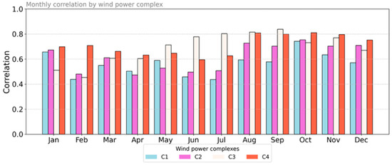
Figure 3.
Monthly correlation between the observed wind speed (AMT) and wind speed predicted by the WRF model, based on 30 min average data throughout the year 2020. Grouped bars represent different wind power complexes. Each group of bars corresponds to a month, and bar height indicates the Pearson correlation coefficient (r), constrained to the [0, 1] interval. Higher values reflect greater agreement between the model predictions and observations.
Figure 4 was designed so that higher values on the Y-axis represent greater correlation, while values closer to zero on the X-axis indicate lower errors. Thus, towers or complexes located near 1 on the Y-axis and near 0 on the X-axis (upper-left region) exhibited the best performance indicators, reflecting high correlation and low errors. Conversely, locations near zero on the Y-axis and farther to the right on the X-axis (lower-right region) showed the poorest performance, characterized by low correlation and high errors. Locations in the lower-left quadrant indicate low correlation with relatively low errors, while those in the upper-right quadrant combine high correlation with high error values. Similar approaches combining error and correlation metrics have been employed in model evaluation studies [84,85]. The results reveal considerable spatial variability in forecast performance, indicating that the model skill varies significantly across locations. This dispersion highlights the influence of local factors, such as topography, land–sea contrast, and surface roughness, on the ability of WRF to represent the wind dynamics [52,64].
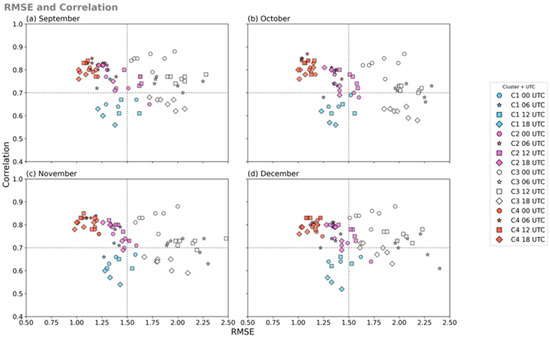
Figure 4.
Scatterplot between the root mean square error (RMSE) and correlation for the observed and simulated data by tower from September to December. Each subplot (a–d) represents one month and includes results for four daily time steps: 00 UTC (circle), 06 UTC (star), 12 UTC (square), and 18 UTC (diamond). Colors indicate tower clusters based on location: C1 (light blue), C2 (purple), C3 (light gray), and C4 (red).
The results indicate that the highest correlations occurred in regions farther from the coastline (Figure 3). Complex C3 consistently reached values close to 0.9, while C4 showed correlations around 0.8 in most months. Wind energy complexes located closer to the coast showed lower correlations, between 0.6 and 0.7, with C1 recording the lowest values among all sites. In contrast, analysis of the RMSE revealed that C3 presented the highest errors, while the remaining complexes performed similarly, with RMSE values between 1.0 and 1.5 m·s−1.
Among the forecast cycles, the 00 UTC run showed the best performance, with a tighter cluster of points, higher correlations (above 0.75), and lower RMSE (typically <1.5 m·s−1), indicating greater consistency during this initialization. In contrast, the 18 UTC run displayed a wider spread, with some stations showing weaker agreement with the observations. Despite these differences, the overall performance remained relatively stable, with most sites achieving correlations between 0.65 and 0.85. The intra-day variability observed may be linked to diurnal atmospheric processes not fully represented by the model, especially under varying boundary-layer conditions. Figure 4 highlights the model performance variability by group and time, emphasizing the joint distribution between error and temporal agreement.
It is essential to evaluate the impact of the forecast update cycles (06, 12, and 18 UTC), as WRF outputs serve as input for other statistical downscaling models within the CER-UFPE wind power forecasting tool. A reduction in input data performance can lead to inaccurate information, propagating errors throughout the simulation. Therefore, it is crucial to carefully assess the cost–benefit of running the model four times per day in conjunction with potential decreases in forecast skill. Figure 5 presents heatmaps of correlation coefficients (top panel) and RMSE (bottom panel) for all anemometric measurement towers (AMTs) evaluated, covering four forecast cycles (00, 06, 12, and 18 UTC) over the months of September, October, November, and December. This figure offers a comprehensive spatiotemporal summary of WRF model performance across the whole set of AMTs (20 AMTs, each AMT belonging to a different wind farm).
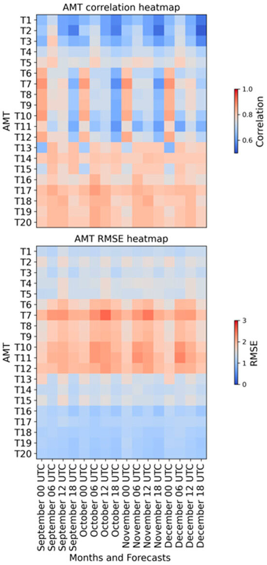
Figure 5.
Heatmap of correlation (top) and RMSE (bottom) for forecast runs and operational months of the WRF model.
The correlation heatmap revealed relatively homogeneous performance across most sites and runs, with values generally ranging from 0.65 to 0.85. Subtle temporal variations were observed, with correlations tending to be slightly higher during September, particularly at the T6, T7, T8, T9, T10, T11 and T12 towers (C3), indicating enhanced forecast skill at the beginning of the austral spring. In contrast, a modest decline in correlation was noted in December across several sites, likely linked to seasonal transitions affecting boundary-layer stability and mesoscale wind regimes. These discrepancies may be associated with terrain-induced variability, since the region is located on a plateau at approximately 1000 m above sea level, displaying higher errors, with RMSE values reaching up to 2.58 m/s. Additionally, the region is surrounded by semiarid areas, while the locality has a more temperate climate compared with its surroundings. However, it is worth noting that even with a considerably higher error compared with the other locations, it is noticeable that the correlations in the region showed good results, suggesting a systematic overestimation bias that could be corrected using post-processing techniques. Regarding the 06, 12, and 18 UTC forecasts, the results showed a significant performance loss, with the lowest correlation values observed in the 18 UTC forecast. However, the RMSE values were not sensitive to changes in the initial and boundary conditions, exhibiting approximately similar values across the forecasts, with the most pronounced variations occurring between months.
In the towers associated with the C1 wind complex, a lower correlation was observed compared with the other complexes. Additionally, a performance loss was evident in T2 when using the 18 UTC cycle of the GFS model. However, a stronger correlation was observed in the 00 UTC cycle. In terms of RMSE, however, the model showed reasonably accurate predictions, with values close to the observed mean. Regarding towers T4, T5, T13, T14, and T15 (C2), the correlations showed slightly higher values compared with C1, with T5 exhibiting slightly higher values in the 06 UTC cycle. However, a decrease in correlations was noticeable in the 12 and 18 UTC cycles. In contrast, the anemometric towers located in C2 showed an RMSE like that of C1.
Towers located in the C4 (T16 to T20) complex consistently exhibited a lower RMSE value typically below 1.2 m/s and high correlations, suggesting high forecast accuracy in these relatively flat and less topographically complex areas. Furthermore, the results for the towers located in C4 showed greater homogeneity in terms of correlation and RMSE with respect to the cycles of initial and boundary data, exhibiting minimal variation in the model’s performance across these updates.
The following sections present the specific results for each wind farm complex. Since WRF is a mesoscale model, the AMTs were grouped by proximity into four complexes, which were analyzed according to their respective locations. Figure 6 illustrates the time series of the average observed and forecasted wind speed across complexes C1 to C4. A low-pass filter was applied to allow for the identification of low-frequency patterns, while the summary tables were calculated using 30 min time series data. All WRF forecasts were bias-corrected using a statistical method (Figure 6), whereby the systematic error at each 30 min interval was removed based on the mean error from the 30 days preceding the forecast.
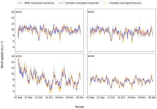
Figure 6.
Time series of the observed (blue) and WRF bias-corrected modeled (orange) wind speed averages for the four wind power complexes. The shaded gray area indicates intra-cluster variability, defined by the minimum and maximum observed values at each time step. Data were smoothed with a 24 h low-pass filter. The analysis covered September–December 2020, with 24 h forecasts initialized at 00 UTC.
In C1, the average wind speeds were around 10 m·s−1, with sporadic reductions (e.g., October 11 and 31, and November 20). After bias correction, the model accurately reproduced these minima. Towers within the complex exhibited marked variability relative to the mean, particularly in September, early October, and November, indicating strong local influences that limited model accuracy at the given resolution. In C2, located 6.5 km from the coastline and sharing similar characteristics with C1, the observed minima were also captured. However, intra-complex variability was smoother than in C1, reflecting more homogeneous wind behavior among towers. In C3, situated more than 400 km inland in elevated semiarid terrain, wind speeds peaked in September and declined through December, consistent with the seasonal transition from dry to rainy periods. Variability across towers was low, suggesting local homogeneity. Forecasts captured both the maxima and minima with good correspondence to the observations. In C4, the average wind speeds were about 8 m·s−1, with the model successfully capturing extreme values. This complex displayed the lowest variability among towers, reinforcing its relative homogeneity compared with the other sites.
Figure 7 shows that the WRF model reproduced the predominant wind directions in all four complexes (C1–C4), but had limitations in representing secondary components, particularly in regions with more complex wind regimes. In C1 and C2, the dominant easterly flow was well-captured, though minor contributions (e.g., ~10% of north–northeast winds in C1) were not represented. C3 exhibited the greatest directional variability, with winds spanning nearly all quadrants, which reduced the model’s accuracy in simulating the full range of observed behavior. In contrast, C4 was more homogeneous, with southeast as the prevailing direction, though the model underestimated finer variations within the southern and eastern quadrants.
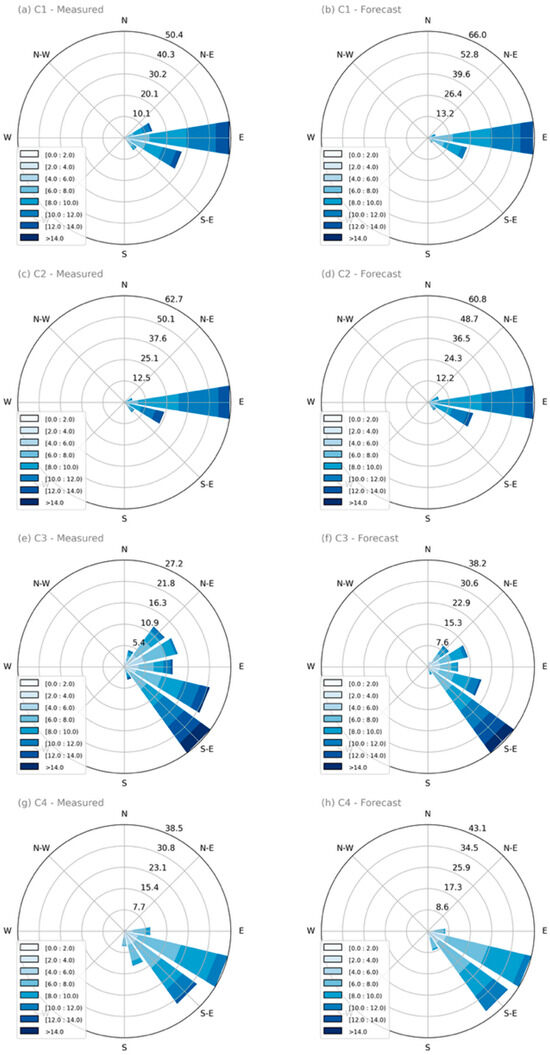
Figure 7.
Wind rose diagrams for the observed and modeled wind data from four meteorological tower complexes (C1 to C4), covering the period from September to December 2020. Subfigures (a,c,e,g) correspond to the observed data (AMT), while (b,d,f,h) show the wind forecasts produced by the WRF model. The wind roses were generated using 30 min interval data, considering wind speeds between 0 and 30 m/s and directions from 0° to 360°, with outliers removed. Each row in the matrix represents a distinct complex, enabling direct comparison between the angular distribution of the observed and modeled winds.
The analysis of Table 3 indicates that the WRF model showed varying performance across the four wind complexes. For each complex, the tower data were averaged, and statistical bias removal was applied, which both enabled the estimation of potential energy generation and attenuated localized effects, thereby improving the mesoscale model performance.
Table 3.
Performance metrics of the WRF model with statistical bias correction for simulating the average wind speed across complexes C1 to C4 from September to December 2020. The columns present the monthly values for the MBE (mean bias error between forecast and observation), MAE (mean absolute error), standard deviation ratio (ratio of the standard deviations between observed and simulated data), RMSE (root mean square error), nRMSE (normalized RMSE), and correlation (correlation coefficient between observed and simulated time series). The normalized values (nRMSE) are expressed as percentages for relative comparison across complexes and months.
In C1, located ~500 m from the coastline, correlation values were the lowest among the complexes (0.62–0.79). Nevertheless, error metrics remained satisfactory, with MBE between −0.03 (December) and 0.13 m·s−1 (September), MAE around 0.88–0.98 m·s−1, and nRMSE between 11 and 13%. These results suggest that the proximity to the sea hampers the model’s ability to capture high-frequency variability, though the mean behavior was well-represented. In C2, with towers 2.5–6.5 km inland, correlation improved markedly (0.80–0.85) compared with C1, highlighting the challenge posed by the land–sea transition. MBE values ranged from 0.00 to 0.17 m·s−1, MAE from 0.83 to 1.05 m·s−1, and nRMSE from 9.77 to 11.56%. The ratio of standard deviations (0.83–1.05) was like that of C1. In C3, located over 400 km inland on a semiarid plateau (~400 m a.s.l.), the performance was more variable, with correlations ranging from 0.71 (December) to 0.89 (September). Error metrics showed greater dispersion (MBE −0.20 to 0.30 m·s−1; MAE 1.12–1.37 m·s−1; nRMSE 10.35–13.05%). Despite this variability, the ratio of standard deviations (0.99–1.09) indicated consistent representation of wind variability. In C4, ~50 km inland at an ~70 m altitude, the model exhibited the best overall performance. Correlations ranged from 0.82 to 0.86, with MBE between −0.10 and 0.05 m·s−1, MAE of 0.74–0.76 m·s−1, and nRMSE of 9.17–11.05%. The ratio of standard deviations (0.94–1.00) confirmed strong consistency between the observations and forecasts.
Table 4 presents the results after bias correction using a machine learning approach, in which hyperparameters were optimized with the Optuna framework for each complex. This method, based on historical WRF forecasts and local measurements, represents the simplest AI technique embedded in the CER-UFPE wind power forecasting tool. More advanced approaches from the statistical downscaling module were beyond the scope of this study. The comparison demonstrates that even simple bias-correction methods can substantially improve the WRF accuracy and realism without the computational expense of increasing WRF model resolution.
Table 4.
Performance metrics of the WRF model with IA bias correction for simulating the average wind speed across complexes C1 to C4 from September to December 2020. The columns present the monthly values for MBE (mean bias error between forecast and observation), MAE (mean absolute error), standard deviation ratio (ratio of the standard deviations between observed and simulated data), RMSE (root mean square error), nRMSE (normalized RMSE), and correlation (correlation coefficient between observed and simulated time series). The normalized values (nRMSE) are expressed as percentages for relative comparison across complexes and months.
When comparing the results between the simple statistical method and the AI-based approach, the latter consistently yielded more satisfactory error metrics across nearly all wind complexes. However, some metrics indicated that the approach was not entirely effective, such as the deviation ratios, which deteriorated across all complexes, suggesting the need for alternative methods to correct these discrepancies. In terms of correlations, the AI approach consistently matched or outperformed the statistical approach for the C2, C3, and C4 complexes, while C1 showed a decline in performance in September (minor loss) and October (significant loss), but with considerable improvement in November and slight improvement in December.
The most notable improvements with the AI approach compared with the simple statistical correction were observed in the MBE, MAE, and nRMSE, showing greater consistency and lower error values. The results indicate that for bias removal, the primary objective of this approach was achieved, and the models provided satisfactory outcomes; however, the variability and standard deviation had lower sensitivity to the bias correction IA models’ approach. Therefore, there is a clear need to enhance the strategies employed to optimize results across disparate points. Consequently, the CER-UFPE wind power forecasting tool offers more complex methodologies for further refinement of WRF-related outputs, including spatial bias removal, through advanced statistical techniques and more robust neural networks.
4. Concluding Remarks
Mesoscale modeling plays a crucial role in dynamically downscaling forecasts from general circulation models (GCMs), embedding regional-scale physical characteristics to improve the forecast accuracy [86]. In this study, the Weather Research and Forecasting (WRF) model was applied over the entire Northeast Brazil (NEB) region, a domain choice aimed at capturing mesoscale atmospheric processes. The WRF model’s capacity to simulate mesoscale features, shaped by topography, land use, and coastline effects, is key to improving deterministic weather predictions [87]. A central objective of this work was to minimize forecast errors through targeted configurations and post-processing, ensuring accurate outputs for automatic meteorological towers (AMTs) while supporting the development of regional forecasting tools. Forecast reliability in deterministic models is closely tied to the accuracy of the initial conditions [48]. In data-scarce regions such as the NEB, limited observational coverage constrains realism, often leading to error propagation throughout simulations.
The strategies employed spectral nudging for data assimilation, integration of high-resolution geographic datasets (MapBiomas, SRTM), and sensitivity testing for optimized parameterizations, which proved effective in forecast skill. Spectral nudging enhances coherence between large- and mesoscale dynamics, while land-use and topographic refinements optimize the representation of surface processes [47,88]. Model configuration required balancing accuracy and computational efficiency: simulations at a 9 km horizontal resolution provided a suitable compromise, maintaining mesoscale fidelity at an acceptable computational cost [89]. Sensitivity analyses confirmed that parameterizations remain a critical source of uncertainty [90], and careful tuning is essential for capturing both convective and stable regimes.
Performance analysis across the four wind complexes revealed heterogeneous results shaped by local characteristics. C1, located ~500 m from the coast, showed the lowest correlations (0.62–0.79), reflecting the difficulty of capturing high-frequency variability induced by land–sea interactions. C2, 2.5–6.5 km inland, achieved correlations between 0.80 and 0.85, while C3, over 400 km inland on a semi-arid plateau, reached values near 0.9 but also showed the highest RMSE (~1.37 m·s−1), and a high correlation variability through the months, highlighting the role of local seasonality. C4, ~50 km inland with simpler terrain, exhibited the most stable and balanced performance, with correlations of 0.82–0.86 and low RMSE (0.74–0.76 m·s−1). These contrasts between the wind energy complexes underscore the influence of topography, coastal transitions, and surface roughness on forecast skill.
Bias correction, including simple machine learning approaches with optimized hyperparameters, further enhanced forecast realism. By removing systematic errors, the correlation values increased, and intra-complex variability was better represented. Even relatively simple AI-based post-processing techniques proved cost-effective, improving the accuracy without the computational burden of higher-resolution runs. Overall, the integration of spectral nudging, land-surface refinement, parameter tuning, and bias correction provided a comprehensive and cost-effective modeling framework for NEB. The high temporal fidelity and spatial consistency obtained from 20 AMTs, unprecedented in operational wind energy studies for the region, offered a robust validation dataset, enabling a uniquely detailed evaluation. In contrast to studies limited to coarse reanalysis or sparse validation, this work demonstrates the value of combining mesoscale modeling with ground-based high-frequency data. As Brazil’s wind energy sector expands, cost-effective calibrated modeling frameworks such as the one presented here will be essential for operational forecasting, reliable grid integration, and climate-resilient energy planning.
Author Contributions
Conceived the idea, Formal analysis, Investigation, Writing—review and editing T.S. and A.C.; Methodology, T.S., A.C., R.W., J.V.d.S.J., L.H.B.A., P.T. and M.F.S.d.L.; Validation, T.S., R.W., J.V.d.S.J., L.H.B.A., P.T., M.F.S.d.L., and H.R.B.d.S.; Formal analysis, A.C. and O.C.V.; Investigation, T.S., A.C., O.C.V., R.W., P.T., and D.V.; Writing—original draft, T.S.; Writing—review and editing, T.S., A.C., O.C.V., R.W., J.V.d.S.J., L.H.B.A., P.T., M.F.S.d.L., H.R.B.d.S., and D.V.; Supervision, D.V. All authors have read and agreed to the published version of the manuscript.
Funding
This research was funded by the National Council for Scientific and Technological Development (CNPq), Brazilian National Power Agency (ANEEL) R&D Program: project PD-00622-0120 (funded by JAURU, CESC and CEC), project PD-00063-3090 (funded by CPFL), and project PD-00048-0217 (funded by CHESF ELETROBRAS). The APC was funded by CNPq grant number 406707/2022-7.
Data Availability Statement
The data used in this study were obtained from meteorological towers managed by a private wind energy company. Due to confidentiality agreements and data ownership restrictions, these datasets cannot be made publicly available. Derived results presented in this manuscript are fully described in the text, figures, and tables. Additional methodological details are available from the corresponding author upon reasonable request.
Acknowledgments
The authors would like to express their gratitude for the financial support by the following projects in the frame of the Brazilian National Power Agency (ANEEL) R&D Program: project PD-00622-0120 (funded by JAURU, CESC and CEC), project PD-00063-3090 (funded by CPFL), and project PD-00048-0217 (funded by CHESF ELETROBRAS). The authors also thank the National Council for Scientific and Technological Development (CNPq) for supporting the SIMOPEC Project—Operational Coupled Ocean–Atmosphere Modeling System for Monitoring and Forecasting Climate Extremes in Vulnerable Areas of Northeastern Brazil (CNPq Grant No. 406707/2022-7).
Conflicts of Interest
The authors declare no conflicts of interest.
References
- Operador Nacional do Sistema Elétrico (ONS). O Sistema em Números. Programa Mensal de Operação. Available online: https://www.ons.org.br/paginas/sobre-o-sin/o-sistema-em-numeros (accessed on 17 February 2025).
- Agência Nacional de Energia Elétrica (ANEEL). SIGA Sistema de Informação de Geração Aneel. Available online: https://app.powerbi.com/view?r=eyJrIjoiNGE3NjVmYjAtNDFkZC00MDY4LTliNTItMTVkZTU4NWYzYzFmIiwidCI6IjQwZDZmOWI4LWVjYTctNDZhMi05MmQ0LWVhNGU5YzAxNzBlMSIsImMiOjR9 (accessed on 17 February 2025).
- de Jong, P.; Barreto, T.B.; Tanajura, C.A.S.; Kouloukoui, D.; Oliveira-Esquerre, K.P.; Kiperstok, A.; Torres, E.A. Estimating the Impact of Climate Change on Wind and Solar Energy in Brazil Using a South American Regional Climate Model. Renew. Energy 2019, 141, 390–401. [Google Scholar] [CrossRef]
- Carvalho, D.; Rocha, A.; Costoya, X.; deCastro, M.; Gómez-Gesteira, M. Wind Energy Resource over Europe under CMIP6 Future Climate Projections: What Changes from CMIP5 to CMIP6. Renew. Sustain. Energy Rev. 2021, 151, 111594. [Google Scholar] [CrossRef]
- Araújo, J.C.H.; Souza, W.F.d.; Meireles, A.J.d.A.; Brannstrom, C. Sustainability Challenges of Wind Power Deployment in Coastal Ceará State, Brazil. Sustainability 2020, 12, 5562. [Google Scholar] [CrossRef]
- Cacciuttolo, C.; Navarrete, M.; Cano, D. Advances, Progress, and Future Directions of Renewable Wind Energy in Brazil (2000–2025–2050). Appl. Sci. 2025, 15, 5646. [Google Scholar] [CrossRef]
- Gehrke, P.; Goretti, A.A.T.; Ávila, L.V. Impactos Da Matriz Energética No Desenvolvimento Sustentável Do Brasil. Rev. Adm. UFSM 2021, 14, 1032–1049. [Google Scholar] [CrossRef]
- Martinez, A.; Iglesias, G. Climate Change and Wind Energy Potential in South America. Sci. Total Environ. 2024, 957, 177675. [Google Scholar] [CrossRef]
- Souza, N.B.P.; Nascimento, E.G.S.; Moreira, D.M.; Souza, N.B.P.; Nascimento, E.G.S.; Moreira, D.M. Performance Evaluation of the WRF Model in a Tropical Region: Wind Speed Analysis at Different Sites. Atmósfera 2023, 36, 253–277. [Google Scholar] [CrossRef]
- Chkeir, S.; Anesiadou, A.; Mascitelli, A.; Biondi, R. Nowcasting Extreme Rain and Extreme Wind Speed with Machine Learning Techniques Applied to Different Input Datasets. Atmos. Res. 2023, 282, 106548. [Google Scholar] [CrossRef]
- Garcia, D.W.; Reboita, M.S.; Carvalho, V.S.B. Sensitivity Analysis and Performance Evaluation of the WRF Model in Forecasting an Extreme Rainfall Event in Itajubá, Southeast Brazil. Atmosphere 2025, 16, 548. [Google Scholar] [CrossRef]
- Garcia, D.W.; Reboita, M.S.; Carvalho, V.S.B. Evaluation of WRF Performance in Simulating an Extreme Precipitation Event over the South of Minas Gerais, Brazil. Atmosphere 2023, 14, 1276. [Google Scholar] [CrossRef]
- Zhang, J.; Yang, L.; Yu, M.; Chen, X. Response of Extreme Rainfall to Atmospheric Warming and Wetting: Implications for Hydrologic Designs Under a Changing Climate. J. Geophys. Res. Atmos. 2023, 128, e2022JD038430. [Google Scholar] [CrossRef]
- Correia Filho, W.L.F.; De Oliveira-Júnior, J.F.; De Barros Santiago, D.; De Bodas Terassi, P.M.; Teodoro, P.E.; De Gois, G.; Blanco, C.J.C.; De Almeida Souza, P.H.; da Silva Costa, M.; Gomes, H.B.; et al. Rainfall Variability in the Brazilian Northeast Biomes and Their Interactions with Meteorological Systems and ENSO via CHELSA Product. Big Earth Data 2019, 3, 315–337. [Google Scholar] [CrossRef]
- Ramos, D.N.d.S.; Fernandez, J.P.R.; Fisch, G. Evolution of the Planetary Boundary Layer on the Northern Coast of Brazil during the CHUVA Campaign. Atmos. Res. 2018, 203, 298–310. [Google Scholar] [CrossRef]
- Fesquet, C.; Drobinski, P.; Barthlott, C.; Dubos, T. Impact of Terrain Heterogeneity on Near-Surface Turbulence Structure. Atmos. Res. 2009, 94, 254–269. [Google Scholar] [CrossRef]
- Brunsell, N.A.; Mechem, D.B.; Anderson, M.C. Surface Heterogeneity Impacts on Boundary Layer Dynamics via Energy Balance Partitioning. Atmos. Chem. Phys. 2011, 11, 3403–3416. [Google Scholar] [CrossRef]
- Lohou, F.; Lothon, M.; Bastin, S.; Brut, A.; Canut, G.; Cohard, J.-M.; Cheruy, F.; Couvreux, F.; Dupont, S.; Lafont, S.; et al. Model and Observation for Surface–Atmosphere Interactions over Heterogeneous Landscape: MOSAI Project. J. Eur. Meteorol. Soc. 2025, 3, 100019. [Google Scholar] [CrossRef]
- Huang, H.; Margulis, S.A. On the Impact of Surface Heterogeneity on a Realistic Convective Boundary Layer. Water Resour. Res. 2009, 45, W04425. [Google Scholar] [CrossRef]
- Jacobson, M.Z. Fundamentals of Atmospheric Modeling; Cambridge University Press: Cambridge, UK, 2005; ISBN 9780521548656. [Google Scholar]
- Hong, S.-P. Different Numerical Techniques, Modeling and Simulation in Solving Complex Problems. J. Mach. Comput. 2023, 3, 58. [Google Scholar] [CrossRef]
- Dameris, M.; Jöckel, P. Numerical Modeling of Climate-Chemistry Connections: Recent Developments and Future Challenges. Atmosphere 2013, 4, 132–156. [Google Scholar] [CrossRef]
- Lynch, P. The Origins of Computer Weather Prediction and Climate Modeling. J. Comput. Phys. 2008, 227, 3431–3444. [Google Scholar] [CrossRef]
- Gross, M.; Wan, H.; Rasch, P.J.; Caldwell, P.M.; Williamson, D.L.; Klocke, D.; Jablonowski, C.; Thatcher, D.R.; Wood, N.; Cullen, M.; et al. Physics–Dynamics Coupling in Weather, Climate, and Earth System Models: Challenges and Recent Progress. Mon. Weather Rev. 2018, 146, 3505–3544. [Google Scholar] [CrossRef]
- Benavente, N.R.; Vara-Vela, A.L.; Nascimento, J.P.; Acuna, J.R.; Damascena, A.S.; de Fatima Andrade, M.; Yamasoe, M.A. Air Quality Simulation with WRF-Chem over Southeastern Brazil, Part I: Model Description and Evaluation Using Ground-Based and Satellite Data. Urban. Clim. 2023, 52, 101703. [Google Scholar] [CrossRef]
- Figueroa, S.N.; Bonatti, J.P.; Kubota, P.Y.; Grell, G.A.; Morrison, H.; Barros, S.R.M.; Fernandez, J.P.R.; Ramirez, E.; Siqueira, L.; Luzia, G.; et al. The Brazilian Global Atmospheric Model (BAM): Performance for Tropical Rainfall Forecasting and Sensitivity to Convective Scheme and Horizontal Resolution. Weather Forecast. 2016, 31, 1547–1572. [Google Scholar] [CrossRef]
- Freitas, S.R.; Panetta, J.; Longo, K.M.; Rodrigues, L.F.; Moreira, D.S.; Rosário, N.E.; Silva Dias, P.L.; Silva Dias, M.A.F.; Souza, E.P.; Freitas, E.D.; et al. The Brazilian Developments on the Regional Atmospheric Modeling System (BRAMS 5.2): An Integrated Environmental Model Tuned for Tropical Areas. Geosci. Model. Dev. 2017, 10, 189–222. [Google Scholar] [CrossRef]
- Mantovani Júnior, J.A.; Aravéquia, J.A.; Carneiro, R.G.; Fisch, G. Evaluation of PBL Parameterization Schemes in WRF Model Predictions during the Dry Season of the Central Amazon Basin. Atmosphere 2023, 14, 850. [Google Scholar] [CrossRef]
- Holtslag, A.A.M. Introduction to the Third GEWEX Atmospheric Boundary Layer Study (GABLS3). Bound. Layer. Meteorol. 2014, 152, 127–132. [Google Scholar] [CrossRef]
- Huang, L.; Bai, L. Evaluation of Planetary Boundary Layer Schemes on the Urban Heat Islands in the Urban Agglomeration over the Greater Bay Area in South China. Front. Earth Sci. 2023, 10, 1065074. [Google Scholar] [CrossRef]
- Kepert, J.D. Choosing a Boundary Layer Parameterization for Tropical Cyclone Modeling. Mon. Weather Rev. 2012, 140, 1427–1445. [Google Scholar] [CrossRef]
- KoHler, M.; Ahlgrimm, M.; Beljaars, A. Unified Treatment of Dry Convective and Stratocumulus-Topped Boundary Layers in the ECMWF Model. Q. J. R. Meteorol. Soc. 2011, 137, 43–57. [Google Scholar] [CrossRef]
- Krishnamurti, T.N.; Stefanova, L.; Misra, V. Tropical Meteorology: An Introduction; Springer: Berlin/Heidelberg, Germany, 2013; ISBN 978-1461474081. [Google Scholar]
- Mahrt, L. Stably Stratified Atmospheric Boundary Layers. Annu. Rev. Fluid. Mech. 2014, 46, 23–45. [Google Scholar] [CrossRef]
- Sandu, I.; Beljaars, A.; Bechtold, P.; Mauritsen, T.; Balsamo, G. Why Is It so Difficult to Represent Stably Stratified Conditions in Numerical Weather Prediction (NWP) Models? J. Adv. Model. Earth Syst. 2013, 5, 117–133. [Google Scholar] [CrossRef]
- Draxl, C.; Hahmann, A.N.; Peña, A.; Giebel, G. Evaluating Winds and Vertical Wind Shear from Weather Research and Forecasting Model Forecasts Using Seven Planetary Boundary Layer Schemes. Wind. Energy 2014, 17, 39–55. [Google Scholar] [CrossRef]
- Olson, J.B.; Kenyon, J.S.; Djalalova, I.; Bianco, L.; Turner, D.D.; Pichugina, Y.; Choukulkar, A.; Toy, M.D.; Brown, J.M.; Angevine, W.M.; et al. Improving Wind Energy Forecasting through Numerical Weather Prediction Model Development. Bull. Am. Meteorol. Soc. 2019, 100, 2201–2220. [Google Scholar] [CrossRef]
- Pryor, S.C.; Shepherd, T.J.; Volker, P.J.H.; Hahmann, A.N.; Barthelmie, R.J. “Wind Theft” from Onshore Wind Turbine Arrays: Sensitivity to Wind Farm Parameterization and Resolution. J. Appl. Meteorol. Climatol. 2020, 59, 153–174. [Google Scholar] [CrossRef]
- Cruz, M.T.; Simpas, J.B.; Sorooshian, A.; Betito, G.; Cambaliza, M.O.L.; Collado, J.T.; Eloranta, E.W.; Holz, R.; Topacio, X.G.V.; Del Socorro, J.; et al. Impacts of Regional Wind Circulations on Aerosol Pollution and Planetary Boundary Layer Structure in Metro Manila, Philippines. Atmos. Environ. 2023, 293, 119455. [Google Scholar] [CrossRef]
- Han, S.; Hao, T.; Yang, X.; Yang, Y.; Luo, Z.; Zhang, Y.; Tang, Y.; Lu, M. Land-Sea Difference of the Planetary Boundary Layer Structure and Its Influence on PM2.5—Observation and Numerical Simulation. Sci. Total Environ. 2023, 858, 159881. [Google Scholar] [CrossRef] [PubMed]
- Pyykkö, J.; Svensson, G. Wind Turning in the Planetary Boundary Layer in CMIP6 Models. J. Clim. 2023, 36, 5729–5742. [Google Scholar] [CrossRef]
- Powers, J.G.; Klemp, J.B.; Skamarock, W.C.; Davis, C.A.; Dudhia, J.; Gill, D.O.; Coen, J.L.; Gochis, D.J.; Ahmadov, R.; Peckham, S.E.; et al. The Weather Research and Forecasting Model: Overview, System Efforts, and Future Directions. Bull. Am. Meteorol. Soc. 2017, 98, 1717–1737. [Google Scholar] [CrossRef]
- Skamarock, W.C.; Klemp, J.B.; Dudhia, J.; Gill, D.O.; Liu, Z.; Berner, J.; Wang, W.; Powers, J.G.; Duda, M.G.; Barker, D.M.; et al. A Description of the Advanced Research WRF Model Version 4.3; 2021. Available online: https://opensky.ucar.edu/islandora/object/technotes%3A576 (accessed on 20 July 2021).
- Wang, W.; Bruyère, C.; Duda, M.; Dudhia, J.; Gill, D.; Kavulich, M.; Werner, K.; Chen, M.; Lin, H.-C.; Michalakes, J.; et al. Weather Research & Forecasting Model ARW Version 4 Modeling System User’s Guide; EUA: Boulder, CO, USA, 2019. [Google Scholar]
- Otero-Casal, C.; Patlakas, P.; Prósper, M.A.; Galanis, G.; Miguez-Macho, G. Development of a High-Resolution Wind Forecast System Based on the WRF Model and a Hybrid Kalman-Bayesian Filter. Energies 2019, 12, 3050. [Google Scholar] [CrossRef]
- Delfino, R.J.; Bagtasa, G.; Hodges, K.; Vidale, P.L. Sensitivity of Simulating Typhoon Haiyan (2013) Using WRF: The Role of Cumulus Convection, Surface Flux Parameterizations, Spectral Nudging, and Initial and Boundary Conditions. Nat. Hazards Earth Syst. Sci. 2022, 22, 3285–3307. [Google Scholar] [CrossRef]
- Pedruzzi, R.; Andreão, W.L.; Baek, B.H.; Hudke, A.P.; Glotfelty, T.W.; Dias de Freitas, E.; Martins, J.A.; Bowden, J.H.; Pinto, J.A.; Alonso, M.F.; et al. Update of Land Use/Land Cover and Soil Texture for Brazil: Impact on WRF Modeling Results over São Paulo. Atmos. Environ. 2022, 268, 118760. [Google Scholar] [CrossRef]
- Slingo, J.; Palmer, T. Uncertainty in Weather and Climate Prediction. Philos. Trans. R. Soc. A Math. Phys. Eng. Sci. 2011, 369, 4751–4767. [Google Scholar] [CrossRef] [PubMed]
- Wang, H.; Yang, J.; Zeng, Y.; Zhang, Q.; Liu, Y.; Gu, J.; Dietrich, S.; Sun, H.; Wang, H.; Yang, J.; et al. Improving Forecast of Severe Oceanic Mesoscale Convective Systems Using FY-4A Lightning Data Assimilation with WRF-FDDA. Remote Sens. 2022, 14, 1965. [Google Scholar] [CrossRef]
- Bughici, T.; Lazarovitch, N.; Fredj, E.; Tas, E. Evaluation and Bias Correction in WRF Model Forecasting of Precipitation and Potential Evapotranspiration. J. Hydrometeorol. 2019, 20, 965–983. [Google Scholar] [CrossRef]
- Jiménez, P.A.; González-Rouco, J.F.; Navarro, J.; Montávez, J.P.; García-Bustamante, E. Quality Assurance of Surface Wind Observations from Automated Weather Stations. J. Atmos. Ocean. Technol. 2010, 27, 1101–1122. [Google Scholar] [CrossRef]
- Fang, J.; Peringer, A.; Stupariu, M.S.; Pǎtru-Stupariu, I.; Buttler, A.; Golay, F.; Porté-Agel, F. Shifts in Wind Energy Potential Following Land-Use Driven Vegetation Dynamics in Complex Terrain. Sci. Total Environ. 2018, 639, 374–384. [Google Scholar] [CrossRef]
- López-Espinoza, E.D.; Zavala-Hidalgo, J.; Mahmood, R.; Gómez-Ramos, O. Assessing the Impact of Land Use and Land Cover Data Representation on Weather Forecast Quality: A Case Study in Central Mexico. Atmosphere 2020, 11, 1242. [Google Scholar] [CrossRef]
- Luu, L.N.; van Meijgaard, E.; Philip, S.Y.; Kew, S.F.; de Baar, J.H.S.; Stepek, A. Impact of Surface Roughness Changes on Surface Wind Speed Over Western Europe: A Study With the Regional Climate Model RACMO. J. Geophys. Res. Atmos. 2023, 128, e2022JD038426. [Google Scholar] [CrossRef]
- Kendzierski, S. Impact of WRF Model Parameterization Settings on the Quality of Short-Term Weather Forecasts over Poland. Atmosphere 2024, 15, 1425. [Google Scholar] [CrossRef]
- Fernández-González, S.; Martín, M.L.; García-Ortega, E.; Merino, A.; Lorenzana, J.; Sánchez, J.L.; Valero, F.; Rodrigo, J.S. Sensitivity Analysis of the WRF Model: Wind-Resource Assessment for Complex Terrain. J. Appl. Meteorol. Climatol. 2018, 57, 733–753. [Google Scholar] [CrossRef]
- Adomako, A.B.; Yusup, Y.; Elsebakhi, E.; Jaafar, M.H.; Ishak, M.I.S.; Hwee San, L.; Ahmad, M.I. Sensitivity Analysis and Validation of WRF-ARW Parameterizations for Potential Solar and Wind Energy Sources over Malaysia. Weather Forecast. 2024, 39, 1833–1847. [Google Scholar] [CrossRef]
- Keshtgar, M.; Siadatmousavi, S.M. Sensitivity Analysis of WRF Model to Physical Parameterization for the Characterization of Coastal and Offshore Wind Patterns in Caspian Sea Region. Theor. Appl. Climatol. 2025, 156, 10. [Google Scholar] [CrossRef]
- Zhang, T.; Cao, L.; Li, S.; Zhan, C.; Wang, J.; Zhao, T. Comprehensive Sensitivity Analysis of the WRF Model for Meteorological Simulations in the Arctic. Atmos. Res. 2024, 299, 107200. [Google Scholar] [CrossRef]
- Hong, S.; Lim, J. The WRF Single-Moment 6-Class Microphysics Scheme (WSM6). J. Korean Meteorol.-Ical Soc. 2006, 42, 129–151. [Google Scholar]
- Ma, L.M.; Tan, Z.M. Improving the Behavior of the Cumulus Parameterization for Tropical Cyclone Prediction: Convection Trigger. Atmos. Res. 2009, 92, 190–211. [Google Scholar] [CrossRef]
- Kain, J.S. The Kain–Fritsch Convective Parameterization: An Update. J. Appl. Meteorol. 2004, 43, 170–181. [Google Scholar] [CrossRef]
- Iacono, M.J.; Delamere, J.S.; Mlawer, E.J.; Shephard, M.W.; Clough, S.A.; Collins, W.D. Radiative Forcing by Long-Lived Greenhouse Gases: Calculations with the AER Radiative Transfer Models. J. Geophys. Res. 2008, 113, D13103. [Google Scholar] [CrossRef]
- Jiménez, P.A.; Dudhia, J. Improving the Representation of Resolved and Unresolved Topographic Effects on Sur-face Wind in the Wrf Model. J. Appl. Meteorol. Climatol. 2012, 51, 300–316. [Google Scholar] [CrossRef]
- Shin, H.H.; Hong, S.Y. Representation of the Subgrid-Scale Turbulent Transport in Convective Boundary Layers at Gray-Zone Resolutions. Mon. Weather Rev. 2015, 143, 250–271. [Google Scholar] [CrossRef]
- Tewari, M.; Chen, F.; Wang, W.; Dudhia, J.; LeMone, M.A.; Mitchell, K.; Ek, M.; Gayno, G.; Wegiel, J.; Cuenca, R.H. Implementation and Verification of the Unified NOAH Land Surface Model in the WRF Model. In Proceedings of the 20th Conference on Weather Analysis and Forecasting/16th Conference on Numerical Weather Prediction, Seattle, WA, USA, 12–16 January 2004; pp. 11–15. [Google Scholar]
- Von Storch, H.; Langenberg, H.; Feser, F. A Spectral Nudging Technique for Dynamical Downscaling Purposes. Mon. Weather Rev. 2000, 128, 3664–3673. [Google Scholar] [CrossRef]
- von Storch, J.-S. What Determines the Spectrum of a Climate Variable at Zero Frequency? J. Clim. 1999, 12, 2124–2127. [Google Scholar] [CrossRef]
- Miguez-Macho, G.; Stenchikov, G.L.; Robock, A. Spectral Nudging to Eliminate the Effects of Domain Position and Geometry in Regional Climate Model Simulations. J. Geophys. Res. Atmos. 2004, 109, D13104. [Google Scholar] [CrossRef]
- Gómez, B.; Miguez-Macho, G. Spectral Nudging in the Tropics. Earth Syst. Dyn. Discuss. 2020, 1–26. [Google Scholar] [CrossRef]
- Otte, T.L.; Nolte, C.G.; Otte, M.J.; Bowden, J.H. Does Nudging Squelch the Extremes in Regional Climate Modeling? J. Clim. 2012, 25, 7046–7066. [Google Scholar] [CrossRef]
- Bowden, J.H.; Otte, T.L.; Nolte, C.G.; Otte, M.J. Examining Interior Grid Nudging Techniques Using Two-Way Nesting in the WRF Model for Regional Climate Modeling. J. Clim. 2012, 25, 2805–2823. [Google Scholar] [CrossRef]
- Warner, T.T. Quality Assurance in Atmospheric Modeling. Bull. Am. Meteorol. Soc. 2011, 92, 1601–1610. [Google Scholar] [CrossRef]
- Saikrishna, T.S.; Ramu, D.A.; Prasad, K.B.R.R.H.; Osuri, K.K.; Rao, A.S. High Resolution Dynamical Downscaling of Global Products Using Spectral Nudging for Improved Simulation of Indian Monsoon Rainfall. Atmos. Res. 2022, 280, 106452. [Google Scholar] [CrossRef]
- Sun, W.; Liu, Z.; Song, G.; Zhao, Y.; Guo, S.; Shen, F.; Sun, X. Improving Wind Speed Forecasts at Wind Turbine Locations over Northern China through Assimilating Nacelle Winds with WRFDA. Weather Forecast. 2022, 37, 545–562. [Google Scholar] [CrossRef]
- Akiba, T.; Sano, S.; Yanase, T.; Ohta, T.; Koyama, M. Optuna. In Proceedings of the Proceedings of the 25th ACM SIGKDD International Conference on Knowledge Discovery & Data Mining, Anchorage, AK, USA, 4–8 August 2019; ACM: New York, NY, USA, 2019; pp. 2623–2631. [Google Scholar]
- Sayeed, A.; Choi, Y.; Jung, J.; Lops, Y.; Eslami, E.; Salman, A.K. A Deep Convolutional Neural Network Model for Improving WRF Simulations. IEEE Trans. Neural Netw. Learn. Syst. 2023, 34, 750–760. [Google Scholar] [CrossRef]
- Hugeback, K.K.; Gallus, W.A.; Villegas Pico, H.N. Machine Learning–Adjusted WRF Forecasts to Support Wind Energy Needs in Black Start Operations. Weather Forecast. 2023, 38, 1553–1561. [Google Scholar] [CrossRef]
- Liu, Z.; Zhang, J.; Yang, Y.; Wang, Y.; Luo, W.; Zhou, X. Enhancing Weather Forecast Accuracy Through the Integration of WRF and BP Neural Networks: A Novel Approach. Earth Space Sci. 2024, 11, e2024EA003613. [Google Scholar] [CrossRef]
- Zhang, J.; Gao, Z.; Li, Y. Deep-Learning Correction Methods for Weather Research and Forecasting (WRF) Model Precipitation Forecasting: A Case Study over Zhengzhou, China. Atmosphere 2024, 15, 631. [Google Scholar] [CrossRef]
- Liu, H.; Tan, Z.; Wang, Y.; Tang, J.; Satoh, M.; Lei, L.; Gu, J.; Zhang, Y.; Nie, G.; Chen, Q. A Hybrid Machine Learning/Physics-Based Modeling Framework for 2-Week Extended Prediction of Tropical Cyclones. J. Geophys. Res. Mach. Learn. Comput. 2024, 1, e2024JH000207. [Google Scholar] [CrossRef]
- Hu, W.; Ghazvinian, M.; Chapman, W.E.; Sengupta, A.; Ralph, F.M.; Delle Monache, L. Deep Learning Forecast Uncertainty for Precipitation over the Western United States. Mon. Weather Rev. 2023, 151, 1367–1385. [Google Scholar] [CrossRef]
- Gurgel, A.d.R.C.; Sales, D.C.; Lima, K.C. Wind Power Density in Areas of Northeastern Brazil from Regional Climate Models for a Recent Past. PLoS ONE 2024, 19, e0307641. [Google Scholar] [CrossRef]
- Taylor, K.E. Summarizing Multiple Aspects of Model Performance in a Single Diagram. J. Geophys. Res. Atmos. 2001, 106, 7183–7192. [Google Scholar] [CrossRef]
- Willmott, C.; Matsuura, K. Advantages of the Mean Absolute Error (MAE) over the Root Mean Square Error (RMSE) in Assessing Average Model Performance. Clim. Res. 2005, 30, 79–82. [Google Scholar] [CrossRef]
- Schumacher, V.; Fernández, A.; Justino, F.; Comin, A. WRF High Resolution Dynamical Downscaling of Precipitation for the Central Andes of Chile and Argentina. Front. Earth Sci. 2020, 8, 328. [Google Scholar] [CrossRef]
- Giorgi, F.; Mearns, L.O. Introduction to Special Section: Regional Climate Modeling Revisited. J. Geophys. Res. Atmos. 1999, 104, 6335–6352. [Google Scholar] [CrossRef]
- Golzio, A.; Ferrarese, S.; Cassardo, C.; Diolaiuti, G.A.; Pelfini, M. Land-Use Improvements in the Weather Research and Forecasting Model over Complex Mountainous Terrain and Comparison of Different Grid Sizes. Bound. Layer. Meteorol. 2021, 180, 319–351. [Google Scholar] [CrossRef]
- Gnedin, N.Y.; Semenov, V.A.; Kravtsov, A.V. Enforcing the Courant–Friedrichs–Lewy Condition in Explicitly Conservative Local Time Stepping Schemes. J. Comput. Phys. 2018, 359, 93–105. [Google Scholar] [CrossRef]
- Das, M.K.; Das, M.K.; Chowdhury, A.M.; Das, S. Sensitivity Study with Physical Parameterization Schemes for Simulation of Mesoscale Convective Systems Associated with Squall Events. Int. J. Earth Atmos. Sci. 2015, 2, 20–36. [Google Scholar]


Disclaimer/Publisher’s Note: The statements, opinions and data contained in all publications are solely those of the individual author(s) and contributor(s) and not of MDPI and/or the editor(s). MDPI and/or the editor(s) disclaim responsibility for any injury to people or property resulting from any ideas, methods, instructions or products referred to in the content. |
© 2025 by the authors. Licensee MDPI, Basel, Switzerland. This article is an open access article distributed under the terms and conditions of the Creative Commons Attribution (CC BY) license (https://creativecommons.org/licenses/by/4.0/).