Abstract
This study aims to provide an efficient framework for the coordinated integration of AC and DC chargers, intermittent solar Photovoltaic (PV) Distributed Generation (DG) units, and a Distribution Static Compensator (DSTATCOM) across residential, commercial, and industrial zones of a Radial Distribution Network (RDN) considering the benefits of various stakeholders: Electric Vehicle (EV) charging station owners, EV owners, and distribution network operators. The model uses a multi-zone planning method and healthy-bus strategy to allocate Electric Vehicle Charging Stations (EVCSs), Photovoltaic Distributed Generation (PVDG) units, and DSTATCOMs. The proposed framework optimally determines the numbers of EVCSs, PVDG units, and DSTATCOMs using Harris Hawk Optimization, considering the maximization of techno-economic benefits while satisfying all the security constraints. Further, to showcase the benefits from the perspective of EV owners, an EV waiting-time evaluation is performed. The simulation results show that integrating EVCSs (with both AC and DC chargers) with solar PVDG units and DSTATCOMs in the existing RDN improves the voltage profile, reduces power losses, and enhances cost-effectiveness compared to the system with only EVCSs. Furthermore, the zonal division ensures that charging infrastructure is distributed across the network increasing accessibility to the EV users. It is also observed that combining AC and DC chargers across the network provides overall benefits in terms of voltage profile, line loss, and waiting time as compared to a system with only AC or DC chargers. The proposed framework improves EV owners’ access and reduces waiting time, while supporting distribution network operators through enhanced grid stability and efficient integration of EV loads, PV generation, and DSTATCOM.
1. Introduction
The rising use of Electric Vehicles (EVs) has raised the demand for well-planned Electric Vehicle Charging Stations (EVCSs) in Radial Distribution Networks (RDNs). However, large-scale EVCS integration presents technical issues, such as increased actual and reactive power consumption, voltage variations, greater power losses, and transformer and feeder overloading, particularly during peak hours. These consequences can jeopardize the RDN’s dependability and performance, demanding mitigating techniques.
India’s automobile industry is now the world’s fourth largest, and the country has pledged to boost EVs as a signatory to the Paris Agreement [1]. However, a lack of suitable charging infrastructure remains one of the most significant impediments to EV adoption. Infrastructure planning in India is complicated by factors such as inadequate road networks, restricted-electricity RDNs, and dense urban traffic [2]. These reasons highlight the vital necessity of a strong, well-integrated EV charging plan.
To meet these technological and economic hurdles, Distributed Generation (DG) units, particularly Photovoltaic (PV) systems, are being incorporated into the RDN alongside EVCSs. PV-based DG provides localized energy generation, decreasing the load on the main grid, lowering energy losses, and increasing supply sustainability [3]. The instability and intermittent nature of solar power can cause voltage swings, over voltages, and under voltages. These concerns may be more evident in networks with high PV penetration and EV charging demands. To counter these impacts, reactive power compensation devices such as Distribution Static Compensators (DSTATCOMs) are used, which improve voltage stability and power quality. The combination of DSTATCOMs with PV-based DG units improves the voltage profile and mitigates the negative effects of high EVCS penetration [4].
Additionally, a coordinated integration of Photovoltaic Distributed Generation (PVDG) and DSTATCOMs with various EVCS configurations produces an efficient planning infrastructure that improves the RDN’s operating economy, lowers power losses, and increases voltage profiles. The suggested design framework facilitates effective load control while reducing peak demand stress and network instability by strategically incorporating these devices in residential, commercial, and industrial zones. In addition to ensuring dependable and effective EV charging, this integrated strategy supports a more robust and sustainable power distribution infrastructure.
1.1. Literature Review and Research Gap
Recent developments and contributions in this new field of study are highlighted in the section that follows.
The effects of integrating EVCSs with solely AC chargers for EVs within the RDN were examined by the authors in [5]. The effects of including many EV models that were only fitted with DC fast chargers on voltage fluctuation and active and reactive power loss in the Distribution Network (DN) were investigated in [6]. In another study, researchers used stochastic power flow to ideally predict the capacity and position of the EVCSs equipped with only DC chargers and only AC chargers in an RDN [7]. However, the practical deployment of both AC and DC chargers in a combined configuration has not been adequately investigated. Combining both charger types ensures flexible service for diverse EV categories (two-, three-, and four-wheelers) and enhances user satisfaction. The research gap lies in the limited exploration of hybrid AC/DC charger configurations and their planning within the RDN.
The authors of [8,9,10] used a variety of optimization approaches, including Teaching–Learning-Based Optimization (TLBO), Grey Wolf Optimization, and Particle Swarm Optimization (PSO), to suggest EVCS placement solutions. Even though these studies found the best places for charging stations, they frequently led to placements on buses that were adjacent to one another, which resulted in a poor distribution of area and left large areas of the RDN overlooked. Additionally, these studies failed to take into account the network’s zonal division, which is necessary to provide balanced accessibility in various locations. Because AC and DC charging have different power requirements and customer preferences, it is essential to strategically distribute them across different zones in order to enhance grid reliability and user satisfaction. Furthermore, a lot of current research [11,12] ignores pragmatic considerations like choosing appropriate (healthy) buses for EVCS deployment. Achieving extensive network coverage, lowering range anxiety among EV users, and facilitating more effective and scalable EV charging infrastructure planning are the objective of this strategy.
Despite having no tailpipe emissions, EVs indirectly contribute to environmental pollution, since they depend on grid power, which is mostly produced by thermal power plants that use fossil fuels. Reducing greenhouse gas emissions, lowering reliance on conventional sources, and meeting the increasing power demand from EV charging all depend on the RDN’s integration of renewable energy sources [13]. However, the fluctuating nature of solar power often leads to issues such as voltage rise and intermittency [14]. Despite this, limited research has investigated coordinated PV integration in EVCSs across differentiated zones of an RDN.
Several studies [13,14] have developed frameworks for the optimal placement of PV systems and EVCSs in an RDN. Although these studies have provided valuable work related to renewable-integrated EVCS planning, they often neglect the importance of coordinating with reactive power compensation devices.
Reactive power injection is essential for maintaining voltage levels, reducing power losses, and boosting system stability amid increasing EV penetration. Although conventional devices like shunt capacitors and Static Var Compensators [15] have been used to regulate reactive power, they are either not suitable for distribution-level operations or do not have dynamic control capabilities [16]. DSTATCOMs, on the other hand, provide quick and adaptable reactive power assistance, which increases their efficiency in RDNs, particularly when combined with DG and renewable resources [17,18]. There is currently a dearth of thorough study on the comprehensive planning of EVCSs equipped with a combination of AC and DC chargers alongside DG and DSTATCOM, despite the fact that several studies [18,19] have examined the best location and dimensions for DG and DSTATCOM units.
The majority of available research [20] on EVCSs has focused on the optimal locations and capacities of charging stations based on technical and economic characteristics such as voltage profile, power loss, and installation, operation, and maintenance costs. However, less emphasis has been placed on the user-centric statistic of waiting time per EV, which is critical for determining the service quality of a charging station. Long lineups and delays, particularly during peak hours, can dramatically harm the user experience, hinder EV adoption, and cause grid bottlenecks. Although several studies [4,7] recognize the relevance of customer happiness, assessment of EV waiting time under different charger configurations (AC/DC) is still unexplored.
In recent years, soft computing techniques have been particularly helpful for resolving nonlinear real-world problems by meeting inequality and equality criteria [21]. To determine the optimal location and capacity of EVCSs, researchers have employed a variety of optimization methods, including GA [22], PSO [10], and TLBO [8]. However, these approaches suffer from improper balance between the exploration–exploitation phase and have a low rate of convergence. Due to their limited exploration and exploitation capabilities and premature convergence, the traditional optimization techniques [8,10,22] have limitations when used for complex planning problems.
1.2. Contribution
The proposed framework aims to bridge existing gaps and provide an efficient optimization strategy for the comprehensive planning of EVCSs equipped with a combination of AC and DC chargers, PVDG units, and DSTATCOMs in RDNs by addressing significant limitations in the literature. The work overcomes some challenging optimization problems by utilizing Harris Hawk Optimization (HHO), a metaheuristic approach. The MATLAB program is used for implementation, which allows for accurate simulation, system-level assessment, and RDN decision-making. The following are this work’s main contributions:
- The present work aims to optimally determine the distribution of EVCSs, PVDG units, and DSTATCOMs using HHO, considering key techno-economic factors while satisfying all the system security constraints.
- In order to develop a practical planning framework, the types of chargers (i.e., AC and DC) are allocated based on the load characteristics of the network (i.e., residential, commercial, and industrial load).
- To achieve fair and effective resource distribution, the suggested planning framework incorporates a zonal division approach into the RDN. For EV users, this zonal-planning strategy seeks to improve accessibility and lessen range anxiety.
- To make the planning more practical, uncertainties related to PVDG are considered. Additionally, a realistic objective function is developed to minimize energy loss cost, investment cost, and operation and maintenance cost. The feasibility of the plan from the EV users’ perspective is also evaluated by analyzing the waiting time of EVs at charging stations.
2. Mathematical Model
The following section is a discussion of the mathematical modelling of solar PVDG units, DSTATCOMs, and an EVCS. These models are crucial for precisely assessing how each component affects voltage profiles, power flows, and system losses in the RDN. The formulations include real and reactive power injections and operational constraints to reflect realistic system behaviour. Figure 1 illustrates a single line diagram of an RDN incorporating an EVCS, DG, and DSTATCOM. The diagram shows the connection between two buses (Bus t and Bus t + 1) in a power system, including a DG, a DSTATCOM device, and an EVCS. The represents voltage magnitude and phase angle at Bus t, ∠ represents voltage magnitude and phase angle at Bus t + 1, and power flows from Bus t to Bus t + 1 through a distribution line with losses represented by (). At Bus t + 1, several components interact: DG supplies power () to the system, and the EVCS draws power () to charge EVs. The diagram represents a DN, the DG injects real power at Bus t + 1, an EV charging station at Bus t + 1 consumes power, a DSTATCOM device at Bus t regulates reactive power, and the line impedance and current between the buses influence power flow and voltage drop.
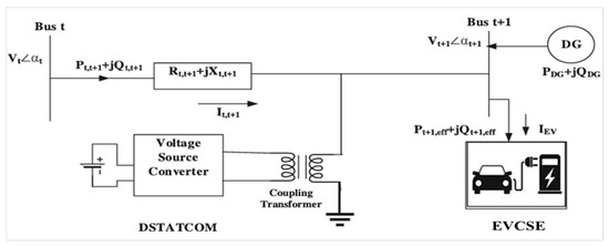
Figure 1.
Single line diagram of RDN with an EVCS, PVDG units, and DSTATCOMs.
2.1. EVCSs Modelling
It is crucial to precisely model EVCSs as part of the load profile in order to facilitate the large-scale integration of EVs into the power system. Depending on the various chargers used in the charging station, an EVCS is considered an additional load to the system’s demand. In this paper, the EVCS is regarded as a continuous power load for modelling purposes, drawing real power for charging processes while not supplying any power to the grid. The number of chargers, their rating, and usage trends, all affect an EVCS’s real power requirements. In this paper, the load impact of EVCS units varies depending on whether they use AC chargers (10 kW) or DC chargers (50 kW) [23] or a combination of both chargers. The sum of the current base load and the EVCS load is the total load at any bus in the RDN that has an EVCS installed. The modified active load at bus i () with an EVCS is represented mathematically as follows [4]:
where as represents base load power at bus i, and represents the EVCS power at bus i.
2.2. PVDG Modelling
Depending on the amount of incident solar radiation, a solar PVDG module transforms solar energy into electrical power. As stated in (2), a beta probability density function is used to express solar irradiance () to account for this uncertainty:
The expected power of solar irradiation per hour is obtained using (2). To improve accuracy, each hour is divided into a number of states (). Each hour’s solar output is calculated as indicated in (3). is interpreted as 10 in this work.
where as , represents total output power related to a state ‘S’, represents an output power associated with the state , the superscript ‘t’ denotes a time step or a particular state index, represents the function related to at a time, and the subscript pd stands for probability density.
In this work, solar irradiation data for Durgapur [24], located in West Bengal (Latitude 23.5204° N, Longitude 87.3119° E), India, was gathered hourly for five years. The tropic of cancer passes near this location, allowing for good visibility of the four seasons: spring, summer, autumn, and winter. This location has mild weather, with temperatures ranging between 15 °C and 40 °C throughout the year. Photovoltaic irradiance is consistent throughout the year in this test province. The mean and standard deviation of the solar irradiation are determined using historical data from the point. A beta probability density function is then produced, and 10 states each hour are taken into consideration in order to correctly model the change in the Solar energy source. These states were chosen because they offer a high degree of accuracy without adding further complexity.
2.3. DSTATCOM Modelling
Rapid reactive power exchange with the distribution feeder’s connecting node is supported by the DSTATCOM device. A steady-state model of DSTATCOM is used in this work to investigate how DSTATCOM affects the RDN. In this study, DSTATCOM deployment involves subtracting its current injection from its respective bus current in BFS (Backward/Forward Sweep)-based load flow calculations. The modified reactive power at bus i () after integrating DSTATCOM () at those buses can be regarded as follows [17,25]:
It is typically used in the context of RDNs, where DSTATCOMs (Distribution Static Synchronous Compensators) are used for reactive power compensation. Equation (4) represents the modified reactive power demand at a particular node i in a RDN after compensation by a DSTATCOM. is the net (or modified) reactive power demand at node i, is the original reactive power demand at node i (before compensation), is the reactive power supplied by the DSTATCOM installed at node i.
3. Technical Parameters
Assessing the influence of PVDG units and DSTATCOMs coupled with EVCSs with various types of AC/DC chargers on an RDN necessitates a thorough study and analysis of the following technical criteria.
3.1. Total Power Loss
Total power loss in a radial-balanced RDN is an important measure of operational efficiency and network performance. Power losses result from the intrinsic resistance of wires and transformer windings. I2R losses can occur over lengthy feeders, especially in rural or poorly inhabited areas. Minimizing total power loss in a balanced network improves voltage management, reduces energy waste, lowers utilities’ operational costs, and increases system dependability. It also helps delay infrastructure improvements by maximizing existing assets and promotes sustainability goals by minimizing total system power loss. Thus, limiting power loss remains a primary goal in the design and planning of RDN. Mathematically it can be computed as follows:
where indicates the branch resistance. Reactive power, real power, and bus voltage are represented by , , and respectively. The total number of branches is symbolized by .
3.2. Voltage Profile
In a balanced RDN, the variance in voltage magnitudes among various buses is referred to as the voltage profile. Line impedances, load locations, and reactive power flows can all result in voltage dips throughout the feeder, even in a balanced system. The correct functioning of electrical equipment, the reduction in technical losses, and the preservation of overall power quality all depend on maintaining a steady and well-regulated voltage profile. A stable voltage profile promotes system dependability and lessens problems like low voltage, shortened equipment life, and disgruntled customers. When adding new loads, such as EVCSs, it is particularly crucial to assess the voltage profile since these loads might affect voltage levels across the network.
3.3. Waiting Time per EV
Planning for EVCSs should take into account both the EVCSs’ owner profitability and the convenience for EV users during charging. We have evaluated the EV user’s waiting time in order to do this. Two charging modes are supported by each EVCS in this work: DC charging, which is quick, and AC charging, which is sluggish. EVs experience considerable waiting times with AC charging due to its slow charging rate, whereas DC charging significantly reduces waiting times because of its faster charging speed. To improve waiting time for EV customers without wasting resources, an M/M/S queuing system model [7] is implemented in this work, as indicated in (6)–(9):
where is the waiting time for an EV in the queue before charging, represents the average rate at which customers arrive at the station, ε denotes the average service rate of the station, H is the total working hours of the charging station, ct is a representation of EV charging time per day, k is the EVCS index, ρ is the average utilization rate of the EV charging station, is the probability that the charging station is empty, which affects how long a new EV will have to wait, is the number of AC/DC chargers present in the EVCS, and is the total number of EVs per charging station per day.
4. Objective Function and Constraints
This section explains the multiple objective functions utilized to solve the proposed optimization problem while adhering to different equality and inequality constraints.
4.1. Objective Function
The current study aims to reduce the overall planning cost (), which includes the investment cost and total energy loss cost of the test RDN with an EVCS, solar DG, and DSTATCOM over a 10-year planning period:
where represents investment cost, is the energy loss cost, represents installation cost, and is the operation and maintenance cost. , , and are the installation cost of the EVCS, PVDG, and DSTATCOM, respectively.
- (a)
- Total Installation Cost ()
The EVCS installation cost () is represented as follows [4]:
where represents the land cost, corresponds to labour cost, and denotes the construction cost of the th EVCS. and account for the expense of AC chargers and DC chargers, respectively. CRF indicates that cost’s recovery factor for the EVCSs and ‘’ indicates the discount rate.
The following are the expressions for and , which includes the solar PVDG and DSTATCOM’s capacity as well as the associated installation costs:
where and are the cost of installing a solar PVDG and DSTATCOM, respectively. and indicate the capacity of the solar PVDG and DSTATCOM, respectively.
- (b)
- Total Operational Cost ()
The operation and maintenance cost provided by the solar DG () and DSTATCOM (), and the cost of the EV charging station () for ten years are all included in the needed operating and maintenance costs for the EVCS, solar DG, and DSTATCOM as follows [17]:
where ‘H’ represents the total number of hours in a day. represents the total number of chargers and represents the number of planning years for the EVCS. is the power drawn from the grid due to the slow/fast charging of EVs and indicates hourly electricity purchase price from the grid.
- (c)
- Total Energy Loss Cost ()
This study aims to minimize the energy loss cost , an important factor for improving efficiency and conserving resources in power system planning. The cost due to energy losses is expressed as follows [17]:
where is the total power losses of the system.
4.2. Constraints
The following equality and inequality constraints must be satisfied to minimize the objective function as given in (10).
- (a)
- Power balance constraints
The sum of the total active/reactive power demand (/), along with the system’s active/reactive power losses (/), must not exceed the grid’s total active/reactive generation capacity (/) as shown below:
- (b)
- Power flow constraints
The power flowing through each network line () should not surpass its maximum allowable limit () to ensure the safe and reliable operation of the power system, as specified by the following criteria:
- (c)
- Voltage constraints
The voltage at each bus () must be maintained within a specified range, restricted by the minimum () and maximum () allowable values, as described below:
- (d)
- Power factor constraints
During operation, the power factor must be kept within an appropriate range, as illustrated below:
5. Problem Formulation
This study examines the challenge of deploying solar PVDG units, various types of EV chargers installed in an EVCS, and DSTATCOMs in an RDN. The input parameters include economic aspects (such as investment and operational expenses), electricity prices, probabilistic solar irradiance models, line and load data of the DN, and devices’ technological limits. To reduce range anxiety, the sites of all devices are carefully chosen utilizing zonal division and a healthy bus strategy for the network. The output parameters of the proposed optimization approach are appropriate locations and optimal sizing for PVDG units, EVCSs (with AC and DC chargers), and DSTATCOMs to improve network performance and economic feasibility. This problem is handled by considering the following objectives:
- i
- Minimization of total installation cost of all devices.
- ii
- Minimization of total operation and maintenance cost of all devices.
- iii
- Minimization of total energy loss cost
With this formulation, the objective has concurrently taken into consideration both technical factors, like reducing power loss, and economic factors. In this work, the objective function is designed to minimize total cost, directly benefitting distribution network operators (DNOs), while also determining the appropriate location of all devices to provide accessibility and convenience, consequently benefiting EV owners.
The following is a description of the optimization framework mathematically:
6. Methodology
The current work provides a robust RDN planning paradigm that takes into account EVCSs, solar PVDG, and DSTATCOM to meet rising EV charging demand and renewable intermittency over a period of 10 years. The HHO approach determines the optimal number of AC and DC chargers for each CS and the number of solar PVDG units and DSTATCOMs allocated in suitable locations of the RDN. The approach for the suggested planning model is detailed below.
6.1. Harris Hawk Optimization Algorithm (HHO)
HHO [26] operates in two main phases: exploration and exploitation. During the exploration phase, hawks thoroughly search different regions of the solution space, while in the exploitation phase, hawks concentrate on refining the high-quality solutions within the search space. In HHO, each hawk represents a possible solution, and the best solution at each step is treated as the target prey or an estimate of the global best. The transition between the exploration and exploitation phases is determined by the value of the escaping energy () as shown below:
If , the program runs the exploration phase; if , the algorithm runs the exploitation phase.
In the exploration phase, hawks update their position based on the following equation:
where , and represent the hawks’ current position, a randomly generated position, and the average position, respectively, while refers to the target or prey’s location. The parameters are randomly generated values within the range 0 and 1. LB and UB denote the lower and upper bounds, respectively, and l denotes the total number of hawks.
The exploitation process consists of four distinct strategies: soft besiege, hard besiege, soft besiege with progressive rapid dives, and hard besiege with progressive rapid dives. In soft besiege, the hawk position will be updated as follows:
where is the difference between the rabbit position and the hawk position. is the jump strength of rabbits.
In hard besiege the hawks update their position using (31):
The soft besiege with progressive rapid dives stage is performed as follows:
where refers to the leavy flight. d and U are the dimensions of the search space and the random vector, respectively.
In hard besiege with progressive rapid dives, the hawk position will update as follows:
6.2. Procedure for Locating the Devices
In this paper, for the benefit of EV owners, the entire RDN is divided into zones that will ensure distributed charging infrastructure. Each use type’s distinct load patterns determine the split into residential, commercial, and industrial zones. In order to plan a realistic situation, buses in residential zones are equipped with AC charges, whereas buses in commercial and industrial sectors are equipped with DC chargers. This strategy provides balanced integration throughout the RDN and guarantees that the charging infrastructure is customized to local usage patterns. For EVCSs and PVDG, the allocation of buses with higher voltage levels and lower active power demands are chosen in each zone, as these buses can accommodate additional load/generation while maintaining voltage stability. For DSTATCOM, deployment buses with higher reactive power demand are chosen in each zone, as these buses are ideal for reactive power compensation without affecting system reliability.
6.3. Implementation of HHO
The HHO method begins by initializing parameters such as population size, decision variables, and maximum number of iterations. In this work, the total population number and maximum iteration size are taken as 50 and 200, respectively. The upper and lower bounds of the number of EV chargers are taken as 15 and 4, the upper and lower bounds of PV capacity are considered to be 300 and 50, and the upper and lower bounds of DSTATCOM are taken as 50 and 10, respectively. The initial solution for EVCSs (), PVDG units (), and DSTATCOMs () is produced in accordance with the size of the population (), which is outlined by the following:
A potential solution to the capacities of EVCSs, PVDG units, and DSTATCOM is described by each set of matrices , , and which are provided as follows:
where , , correspond to the initial capacities of the installed EV chargers equipped with each charging station, PVDG unit, and DSTATCOM, respectively. symbolizes the number of locations in the test system where EVCSs, PVDGs, and DSTATCOMs are installed. In this paper, is taken as 5.
The step-by-step approach to implement the proposed methodology for identifying the optimal locations and capacities of EVCSs and devices is as follows.
Step 1: Read the line data and load data of the RDN, identify the buses with low active and high reactive power demand, and conduct a load flow analysis to evaluate the voltage profile and line loss.
Step 2: Divide the RDN into different zones, namely residential, commercial, and industrial, based on distinct load usage patterns of the users. Allocate DC chargers in commercial and industrial zones and AC chargers in residential zones.
Step 3: As explained in Section 6.2, allocate EVCSs and PVDG units at buses with good voltage profiles and low active power demands in each zone. Similarly, buses with high reactive power demand should be chosen for DSTATCOM allocation.
Step 4: Define the optimization problem as Minimize f(X) as given in (25), where f(X) is the objective function and X is a vector for designed variables.
Step 5: Initialize the population matrices i.e., , , and .
Step 6: Select the best solution () which acts as the hawk’s position for that iteration by evaluation of objective function.
Step7: Calculate the initial energy and escaping energy () of the target using (26) and (27).
Step 8: If ≥ 1, choose the exploration phase, hawks update their position based on (28) and (29).
Step 9: If < 1, choose the exploitation phase, hawks update their position based on (30)–(36).
Step 10: Update the power rating of the EVCSs, PVDG units, and DSTATCOMs.
Step 11: If both the conditions are satisfied in steps 8 and 9, then go to step 12.
Step 12: If convergence criteria is satisfied then print the results; otherwise, go to step 13.
Step 13: Repeat steps 5 through 11 until reaching the stopping criterion, which is the maximum number of iterations
The pseudocode for the HHO algorithm to solve the proposed optimization problem is provided below.
Inputs: The population size and maximum number of iterations
Outputs: The number of EV chargers, PVDG capacity, and DSTATCOM capacity and total cost
Initialize the random population (i = 1, 2,…,)
while (stopping condition is not met) do
Calculate the objective function, i.e., minimization of total cost in terms of installation cost, operational cost, and energy loss cost using (10)–(19)
Set current solution as best solution
for (each vector of decision variables () do
Update the initial energy and jump strength
,
Update the using (26) and (27)
if then ▷ Exploration phase
Update the location vector using (28) and (29)
if then ▷ Exploitation phase
if ) then ▷ Soft besiege
Update the location vector using (30)
else if ) then ▷ Hard besiege
Update the location vector using (31)
else if ) then ▷ Soft besiege with progressive rapid dives
Update the location vector using (32)–(34)
else if ) then ▷ Hard besiege with progressive rapid dives
Update the location vector using (35) and (36)
Return Number of EV chargers, PVDG capacity, DSTATCOM capacity
7. Results and Discussions
This section presents a thorough analysis of the planning results as part of a complete strategy meant to assist DNO in making decisions based on this work.
7.1. Analysis of Test System and Input Data
In this work, for assessing and comparing the findings, a standard IEEE 33-bus test system was used, which contains 33 nodes and 32 connecting branches [27]. The active and reactive power of the 33-bus system was 3.715 MW and 2.3 MVAr, with a base voltage of 12.66 kV. The backward forward sweep method [8] in MATLAB (R2020a) software with an Intel Core i5 CPU and RX-560 GPU, 12th generation was used to perform the load flow of the test network. Table 1 shows the technical parameters and costs of the AC and DC EV chargers used in EVCSs. These charger ratings were obtained from the official e-Amrit portal (a Government of India initiative to promote EV adoption) [23]. This data provides a framework for the realistic modelling and development of EV infrastructure in the RDN.

Table 1.
Ratings of AC and DC Chargers Equipped in EVCSs.
Figure 2 depicts the daily load profile of an EVCS equipped with a level 1 AC charger during a 24 h period [23]. The data shows that peak charging demand occurs between the 20th and 21st hours of a day, most likely owing to customers charging their electric vehicles while returning to home from work. The lowest charging activity is recorded between 1st and 2nd hour of the day, indicating a decrease in user involvement during late-night hours.
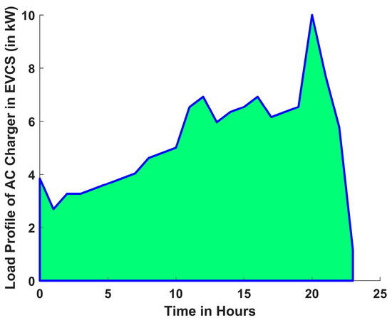
Figure 2.
Load Profile of an EVCS per AC Charger.
Figure 3 depicts the 24 h variation in the load profile of an EVCS that uses a DC charger [23]. The load pattern shows a prolonged peak charging demand between the 8th and 20th hours of the day, which is consistent with commercial and public use, where vehicles are charged during working hours. This high daytime demand indicates a desire for rapid charging options in fleet, taxi, and public charging settings. In contrast, the lowest charging activity occurs between the 0th and 4th hours of the day, when both business and public EV usage is modest. Figure 4 depicts the daily power purchase price from the grid on an hourly basis [28].
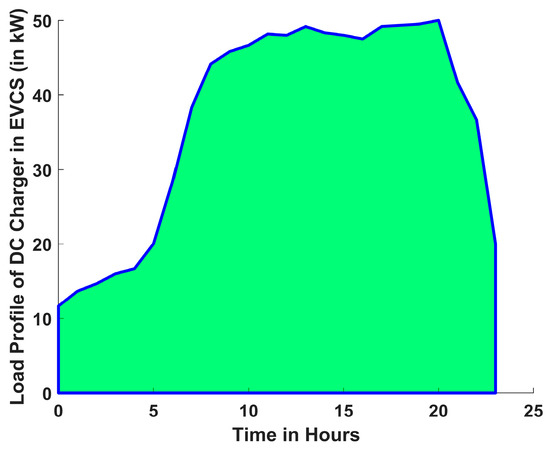
Figure 3.
Load profile of an EVCS per DC Charger.
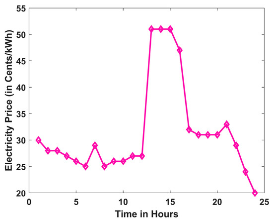
Figure 4.
Hourly electricity purchasing price from the grid.
The above graph depicts the maximum price per unit that emerges between 12 and 14 h. Figure 5 depicts the residential load variance in the 33-bus RDN over a 24 h period. The system interprets peak demand during the tenth hour of the day, with the lowest load occurring between 0 and 3 h. The predicted solar output power curve is derived using the Beta probability density function, as provided in (2) and (3).
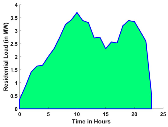
Figure 5.
Residential load variation of 33-Bus RDN.
Figure 6 shows that the peak generating power of solar PV panels fluctuates with the time of day, since solar PV power output is dependent on solar irradiation. The PV panel produces electricity beginning in the morning from 6 to 18 h, with the highest output occurring around noon, as illustrated in Figure 6. All the financial parameters applied in the computation of objective function values for EVCSs with AC and DC chargers, solar PVDG units, and DSTATCOMs are listed in Table 2.
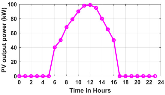
Figure 6.
Solar PVDG hourly power output.
Table 2.
Financial parameters related to AC and DC Chargers in EVCSs, Solar PVDG units, and DSTATCOMs [17].
7.2. Case Description
To prove the efficacy of the proposed charger allocation approach, it is compared with various cases and scenarios. Two primary case studies are carried out in order to assess the effects of various configurations:
Case I: Integration of only EVCSs in the RDN
Case II: Simultaneous integration of EVCSs with PVDG units and DSTATCOMs in the RDN
To evaluate the system’s technical and economic performance, each case is further examined under three different EV charging scenarios:
Scenario 1: EVCSs with AC Chargers
Scenario 2: EVCSs with DC Chargers
Scenario 3: EVCSs with AC and DC Chargers at different locations
7.3. Identification of Locations of EVCSs, Solar PVDG Units, and DSTATCOMs
This section involves a thorough examination of the voltage profiles and power demands of a 33-bus RDN to strategically place DSTATCOMs, solar PVDG units, and EVCSs. Figure 7 shows the voltage profile of the 33-bus RDN. The voltage levels vary throughout the buses, with some seeing modest dips as a result of load concentration among all the buses. Figure 8 illustrates the basic active and reactive power loading across the buses of the test RDN. In scenarios 1 and 2, buses numbered 2, 6, 10, 20, and 26 were selected for the placement of EVCSs and PVDG units, as these buses exhibited high voltage profiles and low active power demand as observed from Figure 7 and Figure 8. Similarly, buses 8, 24, 28, 30, and 33 were selected for DSTATCOM placement in both scenarios due to their high reactive power demand, as observed from Figure 8. As illustrated in Figure 9, the 33-Bus RDN in Scenario 3 is divided into three zones for residential, commercial, and industrial uses. While buses 21 and 23 in commercial zones and bus 28 in the industrial zone are chosen for EVCSs with DC chargers, buses 2 and 10 in residential areas are chosen for EVCSs with AC chargers. As discussed in methodology Section 6.2, the appropriate locations for EVCSs with different chargers, PVDG units, and DSTATCOMs are chosen as shown in Table 3.
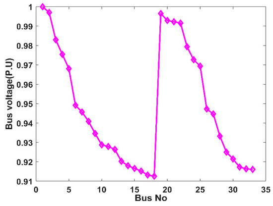
Figure 7.
Voltage profile of 33-bus RDN.
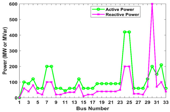
Figure 8.
Base load active and reactive power of 33-bus system.
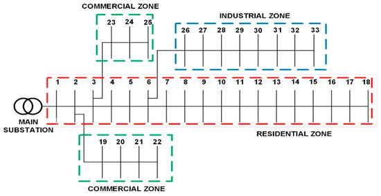
Figure 9.
Single line diagram of IEEE 33-Bus RDN with zone-wise division.
Table 3.
Locations of EVCSs, PVDG units, and DSTATCOMs in Scenario 3.
7.4. Results of Optimal Capacity Determination for All Devices and Objective Function
In this section, EVCSs with various types of chargers, PVDG units, and DSTATCOMs are deployed to achieve optimum capacity in the most suitable locations in the RDN previously determined using Harris Hawk’s Optimization method. Table 4 presents the optimal EVCS capacity for all scenarios in both cases. Table 5 and Table 6 depict the optimal number of chargers at the specified bus numbers in the RDN for all the scenarios in the Case I and Case II configurations, respectively (each charger rating is 10 kW for AC and 50 kW for DC). They also illustrate that the optimal number of chargers accommodated within the 33-bus RDN is higher in Case II, where more EVCSs are combined with solar PVDG and DSTATCOM units than in Case I.
Table 4.
Optimal EVCS capacity for all scenarios.
Table 5.
Optimal capacity and location of EV chargers in Case I.
Table 6.
Optimal capacity and location of EV chargers in Case II.
Further, as observed from Table 5 and Table 6, DC chargers demand more power, owing to their fast-charging capabilities, hence fewer chargers can be safely accommodated. In contrast, the number of AC chargers are high as they consume less power. Table 7 shows that the optimal capacity of the PVDG units and DSTATCOMs that are incorporated into the 33-bus RDN in all scenarios.
Table 7.
Optimal capacity of PVDG units, DSTATCOMs for all scenarios.
The values of the objective functions of scenarios 1, 2, and 3 are the installation cost of EVCSs, PVDG units, and DSTATCOMs, and also the energy loss cost of the EVCSs, PVDG units, and DSTATCOMs, as mentioned in (10)–(27). These values for each case study under different charging scenarios are outlined in Table 8. Table 8 shows that Case II has a higher installation cost than Case I in all scenarios. It is observed from Table 8 that scenario 1 in Case II has the lowest overall cost among all the scenarios. This is because of the low installation cost of AC chargers in scenario 1, as shown in Table 1. Further, it is observed that scenario 2 has the highest overall cost in both cases. It is also observed that despite the higher initial costs of Case II, it consistently yields the lowest overall cost for all the scenarios, proving to be the most economically viable and technically effective strategy for all the scenarios.
Table 8.
Objective values of economical parameters of all scenarios.
7.5. Impact Assessment
Within each case, a thorough comparison of the three planning scenarios is conducted, with an emphasis on important technical indicators like voltage profiles, power losses, and other indicators, such as waiting time. This assessment aids in proving the advantages and efficacy of the suggested optimal integrated planning strategy for EVCSs, solar PVDG units, and DSTATCOMs with different charging infrastructures in RDNs.
- (a)
- Economic Assessment
Table 8 shows the results of the financial analysis for Cases I and II across all scenarios. Despite higher initial investments, the active and reactive power support from PVDG and DSTATCOM, respectively, in Case II, significantly reduce the energy loss cost and operational and maintenance costs, as observed in Table 8. Consequently, Case II offers greater economic benefits compared to Case I. Further it is observed that, in scenario 1, the exclusive presence of AC slow chargers lowers the grid impact and enables superior collaboration with PV and DSTATCOM, making it the most cost-effective option. While Scenario 2 supports fast charging, it leads to higher power losses, increased stress on the RDN, and higher equipment expenses. Scenario 3, with a mix of AC and DC chargers, shows moderate installation and energy loss costs, as well as moderate operation and maintenance costs. This implies that a hybrid setup could offer better overall economic performance than relying solely on DC chargers. In real-world deployments, where cost-effectiveness and performance are crucial factors, this makes Scenario 3 a more sensible and balanced option, because it offers more operational flexibility and moderate investment than Scenario 2.
- (b)
- Voltage Profile Assessment
The voltage profiles of the 33-bus RDN for Scenarios 1, 2, and 3 under Case I and Case II are shown in Figure 10, Figure 11, Figure 12, Figure 13, Figure 14 and Figure 15 throughout a 24 h period. It is clear from these figures that the voltage levels are within allowable bounds in both Case I and Case II for all scenarios. However, the findings clearly show that Case II has a substantially better voltage profile than Case I for all scenarios. These improvements are due to the combined effect of active power injection from solar PVDG units and reactive power assistance from DSTATCOMs. This demonstrates the effectiveness of the coordinated planning of EV infrastructure with PVDG units and DSTATCOMs for maintaining power quality in RDNs. Moreover, it is observed from the figures that the voltage profile in scenario 3 in both cases is better than in scenario 2. This is due to the combined installation of both AC and DC chargers, which ensures more balanced power distribution and enhanced voltage regulation. However, the best voltage profile is achieved in scenario 1, consisting of only AC chargers. The hourly variation in voltage profile at bus 2 of 33-bus system for Cases 1 and 2 is presented in Appendix section, Figure A1.
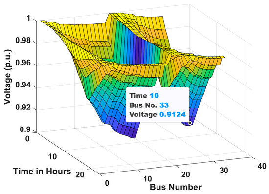
Figure 10.
Voltage profile for Scenario 1 of Case I.
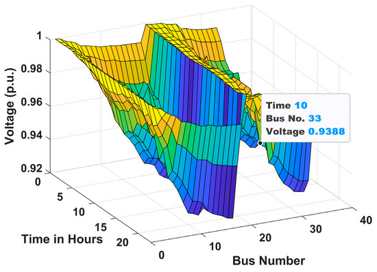
Figure 11.
Voltage profile for Scenario 1 of Case II.
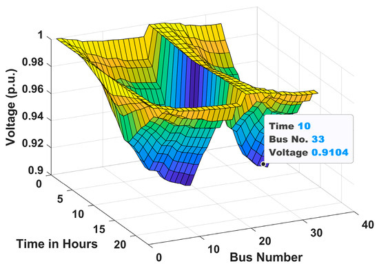
Figure 12.
Voltage profile for Scenario 2 of Case I.
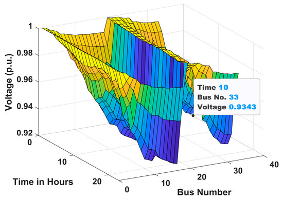
Figure 13.
Voltage profile for Scenario 2 of Case II.
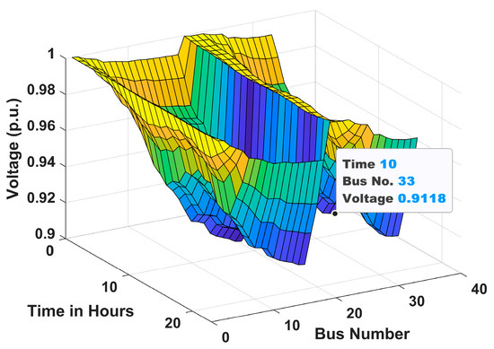
Figure 14.
Voltage profile for Scenario 3 of Case I.
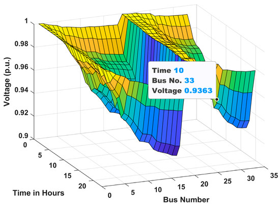
Figure 15.
Voltage profile for Scenario 3 of Case II.
- (c)
- Power Loss Assessment
Figure 16, Figure 17 and Figure 18 present the total active power losses in the 33-bus RDN over 24 h for Scenarios 1, 2, and 3 under Case I. Similarly, Figure 19, Figure 20 and Figure 21 depict the overall active power losses in the 33-bus RDN during a 24 h period for Scenarios 1, 2, and 3 under Case II. In all scenarios it is observed that the maximum power loss occurs in the 10th hour.
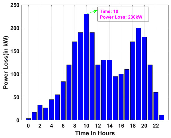
Figure 16.
Power loss for Scenario 1 of Case I.
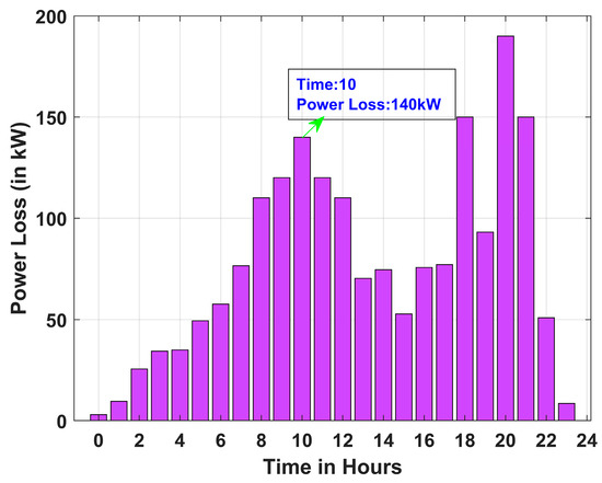
Figure 17.
Power loss for Scenario 1 of Case II.
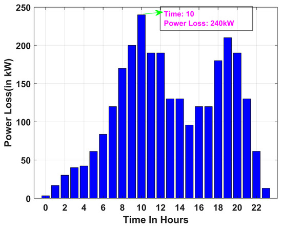
Figure 18.
Power loss for Scenario 2 of Case I.
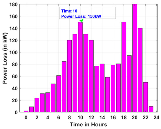
Figure 19.
Power loss for Scenario 2 of Case II.
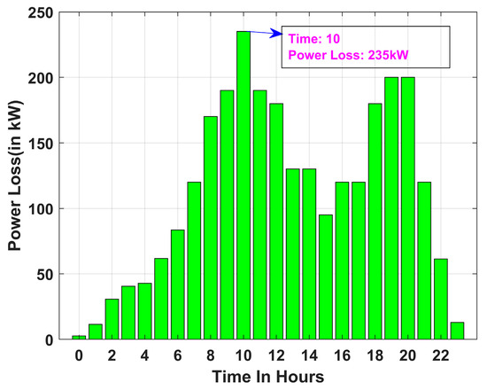
Figure 20.
Power loss for Scenario 3 of Case I.
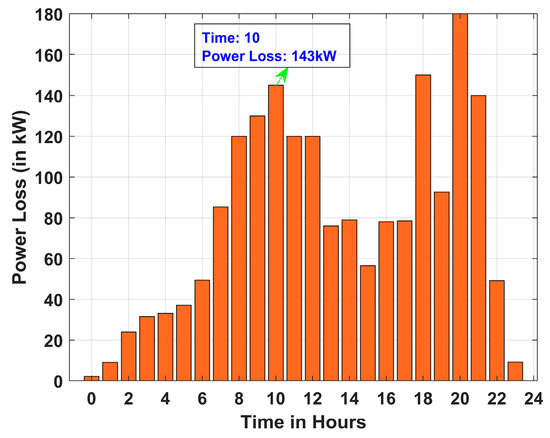
Figure 21.
Power loss for Scenario 3 of Case II.
It is further observed that, across all cases, the maximum power loss occurs in Scenario 2, whereas the minimum power loss is recorded in Scenario 1. Power loss for all scenarios follows the following order: Scenario 1 < Scenario 3 < Scenario 2. Further, it is observed that the incorporation of PVDG and DSTATCOM in Case II aids in the reduction in power loss, as observed from Figure 19, Figure 20 and Figure 21. Hourly variation in line loading and power factor at bus 2 of 33-bus system are provided in Appendix section, Figure A2 and Figure A3, respectively.
- (d)
- Waiting Time Assessment
The waiting time calculation provided in (6)–(9) is used in this part to compare EV waiting times under distinct scenarios. To calculate the average waiting time per EV, it is assumed that each charging station serves a total of 200 EVs per day. The actual arrival rate () of EVs is considered to be 8.33 per hour, whereas the actual service rates () for an AC and DC charger are considered to be 1.76, and 2.81, respectively, for 200 vehicles. The hourly variations in EV arrival rates and service rates that were utilized in the EV waiting time estimation for both AC and DC chargers are presented in Table 9 and Table 10, respectively. The results of the average waiting time for Scenarios 1 and 2 are provided in Table 11. In Scenario 1, only 10 kW AC chargers are installed throughout the RDN. Each EV takes about 6.06 h to completely charge. The slow rate of energy transfer in Scenario 1 causes the waiting time to be much longer. This situation demonstrates the limitations of relying solely on AC chargers to address high-density or widespread EV charging demand, especially in commercial zones or on highways.
Table 9.
Hourly variation in arrival rate utilized in EV waiting time estimation.
Table 10.
Hourly variation in service rate utilized in EV waiting time estimation.
Table 11.
Average waiting time for different chargers.
In Scenario 2, only 50 kW DC chargers are installed in the network. The presence of DC fast chargers in Scenario 2 significantly reduces the waiting time compared to Scenario 1. Therefore, this design provides a far more practical alternative for reducing users’ waiting times and enhancing system responsiveness during peak demand.
Scenario 3 takes a more planned approach, splitting the RDN into functional zones with distinct charger types, such that the residential zone has two AC chargers while the commercial and industrial zones have three DC chargers. Even though the slower AC chargers have a longer waiting time per EV, their use is warranted in residential areas, where EV charging is usually less time sensitive. On the other hand, the installation of DC chargers in the commercial and industrial zones guarantees prompt service, greatly cutting down on waiting times for EV customers.
7.6. Validation of Proposed Method for 28-Bus RDN
To establish the application of the method, the proposed technique is tested on a real Indian 28-bus RDN [29]. The 28-bus system consists of 28 buses and 27 branches, shown in Figure 22, and the total real and reactive power of this system is 829.88 kW and 828.07 Kvar, respectively. For this scenario, 11 Kv and 1 MVA are considered to be the base voltage and base MVA, respectively. As illustrated in Figure 22, the 28-Bus RDN in Scenario 3 is divided into three zones for residential, commercial, and industrial uses. The suitable locations for integrating EVCSs with different chargers, PVDG units, and DSTATCOMs in the system are determined using the methodology described in Section 6.2, and the results are presented in Table 12. Bus 20, located in the commercial zone, and bus 10, situated in the industrial zone, are selected to have EVCSs with DC chargers, while bus 14 in the residential area is chosen to have an EVCS with AC chargers. The results of the objective function of the proposed Scenario 3 are the total costs, including the installation costs and the operation and maintenance costs of the EVCSs, PVDG units, and DSTATCOMs as well as the energy loss cost, which are outlined in Table 13.
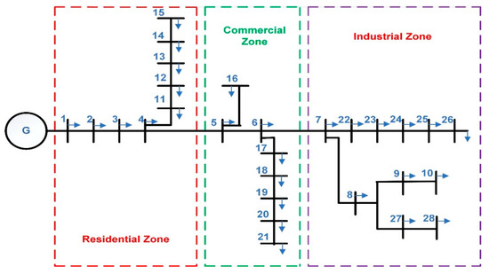
Figure 22.
Single line diagram of Indian 28-Bus rural RDN with zone-wise division.
Table 12.
Locations and optimal sizing of EVCSs, PVDG units, and DSTATCOMs in Scenario 3.
Table 13.
Objective values of economical parameters of scenario.
7.7. Algorithm Comparison
The suggested optimization model focuses on the optimal sizing of the EVCSs (including both AC and DC chargers), PVDG units, and DSTATCOMs. The efficacy of the suggested framework using the proposed HHO algorithm is validated by comparing it with GA, PSO, and the traditional TLBO algorithm. Standard parameter settings are used in each technique for the sake of fair comparison: PSO employs acceleration coefficients (c1 = 1.5, c2 = 1.5) [10] and an inertia weight that decreases linearly from 0.9 to 0.4; GA is set up with a crossover probability of 0.85 and a mutation probability of 0.01 [20]; HHO is intrinsically easier to implement because it does not require algorithm-specific parameter tuning. Normalization is used to provide fair evaluation across all techniques, since the objective function, i.e., , including , , varies greatly in range. This normalized total cost metric is used to compare the algorithms’ convergence characteristics. The convergence properties of HHO, TLBO, PSO, and GA are depicted in Figure 23. The outcomes absolutely suggest that HHO outperforms the other algorithms in terms of convergence speed and overall cost. The good exploration–exploitation balance of HHO is credited with the improved performance.
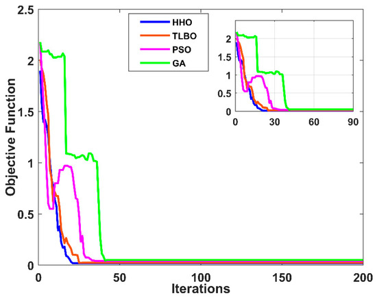
Figure 23.
Comparison of convergence characteristics between different algorithms.
Further, to prove the superiority of the HHO algorithm in solving the proposed problem as compared to other existing algorithms, a detailed comparative analysis is performed, as shown in Table 14 and Table 15. The performance comparison in terms of convergence rate, computational time, mean, and standard deviation between the different algorithms is shown in Table 14. The robustness of the algorithm is evaluated based on the maximum, minimum, and average results after 50 independent runs, as provided in Table 15.
Table 14.
Comparison of results of different algorithms.
Table 15.
Comparison of results of multi-run statistics (50 runs).
Being a minimization problem, the lowest mean and standard deviation values of HHO, as presented in Table 14, demonstrate its superior performance compared to TLBO, PSO, and GA in solving the proposed optimization problem. Moreover, HHO attains the global minimum solution with the least number of iterations, indicating a faster convergence rate.
The robustness of the algorithm was evaluated based on the maximum, minimum, and average objective values obtained from 50 independent runs. As shown in Table 15, the smaller difference between these values in the case of HHO, relative to TLBO, PSO, and GA, further confirms the stability of the HHO algorithm in consistently achieving near-optimal solutions.
Therefore, the results indicate that HHO continuously beats the others in terms of accuracy and convergence speed.
7.8. Sensitivity Analysis
To examine the robustness of the proposed model under different conditions, a sensitivity analysis was carried out by changing the Capital Expenditure (CAPEX) of EV chargers, electricity tariffs, discount rates, EV charger ratings, and number of states in PV uncertainty modelling.
In this analysis, the cost of AC and DC chargers from the original manuscript is considered to be the baseline ( = 941$, = 6850 $), and their CAPEX values are varied by ±25% to assess the impact of cost fluctuations. For the variation in electricity tariffs by ±20%, the tariff profile provided in the original manuscript is considered to be the base case. Further, the discount rate is varied between (6–10%) from its base value of 0.08. Further, the power rating of the EV chargers is varied within practical ranges (±20%) from its base value 50 kW and no. of states in the PV uncertainty modelling is varied between 5, 10, 15, and 20.
The analysis reveals that the model successfully converges, even with variations in critical parameters such as the EV charger ratings and number of states in PV uncertainty modelling. Moreover, the optimization framework consistently reaches feasible and optimal solutions under different parameter settings, demonstrating the robustness of the proposed model. As shown in Table 16, the variation in the CAPEX values of the chargers primarily influences the investment cost, leading to deviations of up to ±22% from the baseline. However, it does not significantly affect the operation and maintenance costs or the energy loss cost. As shown in Table 17, varying the tariff primarily affects the operation and maintenance costs and the energy loss cost, while the investment cost remains unchanged. As presented in Table 18, changing the discount rate affects all components of the total cost—namely, the investment cost, operation and maintenance costs, and energy loss cost.
Table 16.
Results of sensitivity analysis by changing CAPEX value of EV charger.
Table 17.
Results of sensitivity analysis by changing electricity tariff.
Table 18.
Results of sensitivity analysis by changing discount rate.
The impacts on total cost for different charger power ratings for Case I are summarized in Table 19. The results of the sensitivity analysis of PV power output when varying the number of states are shown in Figure 24, Figure 25, Figure 26 and Figure 27. The PV output results obtained for Ns = 5 and 10 showed slight variations, whereas increasing Ns to 15 and 20 yielded PV output results nearly identical to those obtained with Ns = 10. Therefore, Ns = 10 was selected, as it provides a good balance between computational efficiency and accuracy in uncertainty representation. These findings confirm that the proposed model effectively captures the influence of key parameters on the optimization problem and provides optimal solutions.
Table 19.
Sensitivity analysis of power ratings of EV DC fast charger.
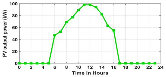
Figure 24.
PV output power obtained by setting the number of states .
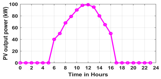
Figure 25.
PV output power obtained by setting the number of states .
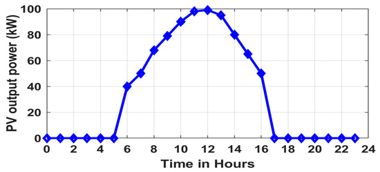
Figure 26.
PV output power obtained by setting the number of states .
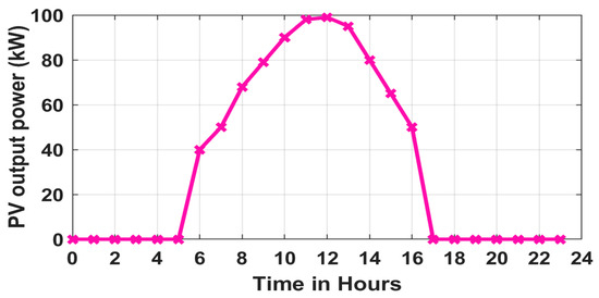
Figure 27.
PV output power obtained by setting the number of states .
8. Conclusions
By combining EVCSs with AC and DC charger types, renewable energy sources, and reactive power compensation devices, this paper aims to maximize techno-economic benefits for EVCS owners, EV owners, and DNOs. The optimal capacities of the PVDG units, AC and DC chargers in EVCSs, and DSTATCOM units were obtained using HHO. The planning framework was optimized by minimizing the system’s overall cost while meeting the security constraints using HHO technique. Economical parameters, like cost, and technical parameters, like hourly voltage profiles, hourly active power losses, and waiting times, have also been evaluated for all cases. Simulations on an IEEE 33-bus RDN were used to validate the suggested approach, and the main conclusions are outlined below.
The key findings of the papers are as follows.
- The combined integration of uncertain solar PVDG units and DSTATCOMs offers both active and reactive power support in an EV-integrated RDN, reducing the grid dependency, thereby significantly lowering the operation and maintenance costs of the system.
- In comparison to Case I, Case II achieved a reduction in energy loss by 38%, 37%, and 39.13% for Scenarios 1, 2, and 3, respectively. In Case II, the voltage profile shows an improvement of 2.89%, 2.63%, and 2.62% for Scenarios 1, 2, and 3, respectively, compared to Case I.
- The zonal division strategy ensures that EVCSs are distributed throughout the network, enhancing overall coverage of the network for EVCS placement. This approach allows more areas to be served with fewer chargers, thereby improving EVCS accessibility for EV users.
- 4.
- Further, the analysis reveals that among Scenarios 1, 2, and 3, the results of , , , and follow the order of Scenario 1< Scenario 3 < Scenario 2 for both cases. This indicates that the combined deployment of both AC and DC chargers in Scenario 3 offers the best balance of operational flexibility and investment cost. As a result, Scenario 3 stands out as the most practical and viable option for real-world implementation.
- 5.
- Additionally, the HHO algorithm outperforms classic TLBO, PSO, and GA in terms of convergence rate and accuracy. It effectively minimizes the total planning costs of EV-, PV-, and DSTATCOM-integrated RDNs, making it suitable for real-world planning challenges.
The primary limitation of the proposed framework is the limited availability of reliable data. In many cases, accurate information on traffic flow, charging behaviour, and local network parameters is unavailable, which can affect the precision and reliability of the model’s outcomes. Furthermore, a fixed-load assumption was adopted for optimization purposes; however, the technical analysis of the proposed model was carried out under variable-load conditions. Future research can include vehicle-to-grid operations and examine how EV charging loads behave dynamically under real-time pricing systems. To guarantee continuous operation and grid security, it is also necessary to incorporate a reliability evaluation of the coordinated system during component failures, cyberattacks, or adverse weather conditions.
Author Contributions
Conceptualization, R.B., S.T., S.R.G., S.C.S. and P.A.; methodology, R.B., S.T., S.R.G. and S.C.S.; software, R.B. and S.T.; validation, R.B., S.T., S.R.G., S.C.S., F.L. and P.A.; formal analysis, R.B., S.T., S.R.G., S.C.S., F.L. and P.A.; writing—original draft preparation, R.B., S.T. and S.R.G.; writing—review and editing, S.R.G., S.C.S., F.L. and P.A.; supervision, S.R.G., S.C.S., F.L. and P.A.; investigation, R.B., S.T., S.R.G., S.C.S., F.L. and P.A. All authors have read and agreed to the published version of the manuscript.
Funding
This research was conducted without any funding from external sources.
Data Availability Statement
The datasets employed in this research, specifically for the 33-bus DN and 28-bus real Indian RDN, are available in [27,29].
Acknowledgments
We sincerely thank the School of Electrical Engineering, KIIT Deemed to be University, Bhubaneswar, for their steadfast support and motivation throughout the course of this study.
Conflicts of Interest
The authors affirm that there are no competing interests associated with this work.
Appendix A. Hourly Variation in Voltage Profile, Line Loading, and Power Factor at Bus 2 of 33-Bus System
The results of Figure A1, Figure A2 and Figure A3 indicate that the integration of PV and DSTATCOM along with the EVCSs in Case 2 improves the voltage profile and enhances the line loading as well as the power factor of the system as compared to Case 1.

Figure A1.
Hourly variation in voltage profile at bus 2 of 33-bus system for both cases.

Figure A2.
Hourly variation in line loading at bus 2 of 33-bus system for both cases.

Figure A3.
Hourly variation in power factor at bus 2 of 33-bus system for both cases.
Table A1.
Line data and bus data of 33-Bus distribution network.
Table A1.
Line data and bus data of 33-Bus distribution network.
| Branch Number | Sending End Bus | Receiving End Bus | Resistance (Ω) | Reactance (Ω) | Active Power (MW) | Reactive Power (MVAr) |
|---|---|---|---|---|---|---|
| 1 | 1 | 2 | 0.0922 | 0.047 | 0.1 | 0.06 |
| 2 | 2 | 3 | 0.493 | 0.2511 | 0.09 | 0.04 |
| 3 | 3 | 4 | 0.366 | 0.1864 | 0.12 | 0.08 |
| 4 | 4 | 5 | 0.3811 | 0.1941 | 0.06 | 0.03 |
| 5 | 5 | 6 | 0.819 | 0.707 | 0.06 | 0.02 |
| 6 | 6 | 7 | 0.1872 | 0.6188 | 0.2 | 0.01 |
| 7 | 7 | 8 | 0.7114 | 0.2351 | 0.2 | 0.01 |
| 8 | 8 | 9 | 1.03 | 0.74 | 0.06 | 0.02 |
| 9 | 9 | 10 | 1.044 | 0.74 | 0.06 | 0.02 |
| 10 | 10 | 11 | 0.1966 | 0.065 | 0.045 | 0.03 |
| 11 | 11 | 12 | 0.3744 | 0.1238 | 0.06 | 0.035 |
| 12 | 12 | 13 | 1.468 | 1.155 | 0.06 | 0.035 |
| 13 | 13 | 14 | 0.5416 | 0.7129 | 0.12 | 0.08 |
| 14 | 14 | 15 | 0.591 | 0.526 | 0.06 | 0.01 |
| 15 | 15 | 16 | 0.7463 | 0.545 | 0.06 | 0.02 |
| 16 | 16 | 17 | 1.289 | 1.721 | 0.06 | 0.02 |
| 17 | 17 | 18 | 0.732 | 0.574 | 0.09 | 0.04 |
| 18 | 2 | 19 | 0.164 | 0.1565 | 0.09 | 0.04 |
| 19 | 19 | 20 | 1.5042 | 1.3554 | 0.09 | 0.04 |
| 20 | 20 | 21 | 0.4095 | 0.4784 | 0.09 | 0.04 |
| 21 | 21 | 22 | 0.7089 | 0.9373 | 0.09 | 0.04 |
| 22 | 3 | 23 | 0.4512 | 0.3083 | 0.09 | 0.05 |
| 23 | 23 | 24 | 0.898 | 0.7091 | 0.42 | 0.2 |
| 24 | 24 | 25 | 0.896 | 0.7011 | 0.42 | 0.2 |
| 25 | 6 | 26 | 0.203 | 0.1034 | 0.06 | 0.025 |
| 26 | 26 | 27 | 0.2842 | 0.1447 | 0.06 | 0.025 |
| 27 | 27 | 28 | 1.059 | 0.9337 | 0.06 | 0.02 |
| 28 | 28 | 29 | 0.8042 | 0.7006 | 0.12 | 0.07 |
| 29 | 29 | 30 | 0.5075 | 0.2585 | 0.2 | 0.06 |
| 30 | 30 | 31 | 0.9744 | 0.963 | 0.15 | 0.07 |
| 31 | 31 | 32 | 0.3105 | 0.3619 | 0.21 | 0.1 |
| 32 | 32 | 33 | 0.341 | 0.5302 | 0.06 | 0.04 |
Table A2.
Line data and bus data of 28-Bus real Indian distribution network.
Table A2.
Line data and bus data of 28-Bus real Indian distribution network.
| Branch Number | Sending End Bus | Receiving End Bus | Resistance (Ω) | Reactance (Ω) | Active Power (MW) | Reactive Power (MVAr) |
|---|---|---|---|---|---|---|
| 1 | 1 | 2 | 1.197 | 0.82 | 35.28 | 35.993 |
| 2 | 2 | 3 | 1.796 | 1.231 | 14 | 14.283 |
| 3 | 3 | 4 | 1.306 | 0.895 | 35.28 | 35.993 |
| 4 | 4 | 5 | 1.851 | 1.268 | 14 | 14.283 |
| 5 | 5 | 6 | 1.524 | 1.044 | 35.28 | 35.993 |
| 6 | 6 | 7 | 1.905 | 1.305 | 35.28 | 35.993 |
| 7 | 7 | 8 | 1.197 | 0.82 | 35.28 | 35.993 |
| 8 | 8 | 9 | 0.653 | 0.447 | 14 | 14.283 |
| 9 | 9 | 10 | 1.143 | 0.783 | 14 | 14.283 |
| 10 | 4 | 11 | 2.823 | 1.172 | 56 | 57.131 |
| 11 | 11 | 12 | 1.184 | 0.491 | 35.28 | 35.993 |
| 12 | 12 | 13 | 1.002 | 0.416 | 35.28 | 35.993 |
| 13 | 13 | 14 | 0.455 | 0.189 | 14 | 14.283 |
| 14 | 14 | 15 | 0.546 | 0.227 | 35.28 | 35.993 |
| 15 | 5 | 16 | 2.55 | 1.058 | 35.28 | 35.993 |
| 16 | 6 | 17 | 1.366 | 0.567 | 8.96 | 9.141 |
| 17 | 17 | 18 | 0.819 | 0.34 | 8.96 | 9.141 |
| 18 | 18 | 19 | 1.548 | 0.642 | 35.28 | 35.993 |
| 19 | 19 | 20 | 1.366 | 0.567 | 35.28 | 35.993 |
| 20 | 20 | 21 | 3.552 | 1.474 | 14 | 14.283 |
| 21 | 7 | 22 | 1.548 | 0.642 | 35.28 | 35.993 |
| 22 | 22 | 23 | 1.092 | 0.453 | 8.96 | 9.141 |
| 23 | 23 | 24 | 0.91 | 0.378 | 56 | 57.131 |
| 24 | 24 | 25 | 0.455 | 0.189 | 8.96 | 9.141 |
| 25 | 25 | 26 | 0.364 | 0.151 | 35.28 | 35.993 |
| 26 | 8 | 27 | 0.546 | 0.226 | 35.28 | 35.993 |
| 27 | 27 | 28 | 0.273 | 0.113 | 35.28 | 35.993 |
References
- Bind, U.; Lamoria, J.P. Customer Adaptation towards Electric Vehicle in Gujarat. Int. J. Res. Publ. Rev. 2025, 6, 1439–1444. [Google Scholar] [CrossRef]
- Kumar, A.; Jadon, J.K.S. A Review on Electric Vehicles and Its Future. S. Asian J. Mark. Manag. Res. 2021, 11, 85–91. [Google Scholar] [CrossRef]
- Adegoke, S.A.; Sun, Y.; Adegoke, A.S.; Ojeniyi, D. Optimal Placement of Distributed Generation to Minimize Power Loss and Improve Voltage Stability. Heliyon 2024, 10, e39298. [Google Scholar] [CrossRef] [PubMed]
- Bonela, R.; Roy Ghatak, S.; Swain, S.C.; Lopes, F.; Nandi, S.; Sannigrahi, S.; Acharjee, P. Analysis of Techno–Economic and Social Impacts of Electric Vehicle Charging Ecosystem in the Distribution Network Integrated with Solar DG and DSTATCOM. Energies 2025, 18, 363. [Google Scholar] [CrossRef]
- Nutkani, I.; Toole, H.; Fernando, N.; Andrew, L.P.C. Impact of EV Charging on Electrical Distribution Network and Mitigating Solutions—A Review. IET Smart Grid 2024, 7, 485–502. [Google Scholar] [CrossRef]
- Sawant, V.; Zambare, P. DC Fast Charging Stations for Electric Vehicles: A Review. Energy Convers. Econ. 2024, 5, 54–71. [Google Scholar] [CrossRef]
- Jin, Y.; Acquah, M.A.; Seo, M.; Han, S. Optimal Siting and Sizing of EV Charging Station Using Stochastic Power Flow Analysis for Voltage Stability. IEEE Trans. Transp. Electrif. 2024, 10, 777–794. [Google Scholar] [CrossRef]
- Abualigah, L.; Abu-Dalhoum, E.; Ikotun, A.M.; Zitar, R.A.; Alsoud, A.R.; Khodadadi, N.; Ezugwu, A.E.; Hanandeh, E.S.; Jia, H. Teaching–Learning-Based Optimization Algorithm: Analysis Study and Its Application. In Metaheuristic Optimization Algorithms; Morgan Kaufmann: San Francisco, CA, USA, 2024; pp. 59–71. [Google Scholar] [CrossRef]
- Golive, S.G.; Paramasivam, B.; Ravindra, J. Optimal Location of EV Charging Stations in the Distribution System Considering GWO Algorithm. Indian J. Sci. Technol. 2024, 17, 751–759. [Google Scholar] [CrossRef]
- Altaf, M.; Yousif, M.; Ijaz, H.; Rashid, M.; Abbas, N.; Khan, M.A.; Waseem, M.; Saleh, A.M. PSO-based Optimal Placement of Electric Vehicle Charging Stations in a Distribution Network in Smart Grid Environment Incorporating Backward Forward Sweep Method. IET Renew. Power Gener. 2024, 18, 3173–3187. [Google Scholar] [CrossRef]
- Kumar, B.V.; Aneesa Farhan, M.A. Optimal Integration of EV Charging Stations and Capacitors for Net Present Value Maximization in Distribution Network. IEEE Lat. Am. Trans. 2025, 23, 239–250. [Google Scholar] [CrossRef]
- Kumar, B.V.; Aneesa Farhan, M.A. Optimal Allocation of EV Charging Station and Capacitors Considering Reliability Using a Hybrid Optimization Approach. Appl. Energy 2024, 375, 124139. [Google Scholar] [CrossRef]
- Rene, E.A.; Fokui, W.S.T. Artificial Intelligence-Based Optimal EVCS Integration with Stochastically Sized and Distributed PVs in an RDNS Segmented in Zones. J. Electr. Syst. Inf. Technol. 2024, 11, 1. [Google Scholar] [CrossRef]
- Kazemi-Robati, E.; Sepasian, M.S.; Hafezi, H.; Arasteh, H. PV-Hosting-Capacity Enhancement and Power-Quality Improvement through Multiobjective Reconfiguration of Harmonic-Polluted Distribution Systems. Int. J. Electr. Power Energy Syst. 2022, 140, 107972. [Google Scholar] [CrossRef]
- Ghatak, S.R.; Basu, D.; Acharjee, P. Voltage Profile Improvement and Loss Reduction Using Optimal Allocation of SVC. In Proceedings of the 2015 Annual IEEE India Conference (INDICON), New Delhi, India, 17–20 December 2015; pp. 1–6. [Google Scholar]
- Ahmadi, B.; Çağlar, R. Determining the Pareto Front of Distributed Generator and Static VAR Compensator Units Placement in Distribution Networks. Int. J. Electr. Comput. Eng. IJECE 2022, 12, 3440. [Google Scholar] [CrossRef]
- Sannigrahi, S.; Ghatak, S.R.; Acharjee, P. Fuzzy Logic–Based Rooted Tree Optimization Algorithm for Strategic Incorporation of DG and DSTATCOM. Int. Trans. Electr. Energy Syst. 2019, 29, e12031. [Google Scholar] [CrossRef]
- Yuvaraj, T.; Ravi, K.; Devabalaji, K.R. Optimal Allocation of DG and DSTATCOM in Radial Distribution System Using Cuckoo Search Optimization Algorithm. Model. Simul. Eng. 2017, 2017, 1–11. [Google Scholar] [CrossRef]
- Karami, H.; Zaker, B.; Vahidi, B.; Gharehpetian, G.B. Optimal Multi-Objective Number, Locating, and Sizing of Distributed Generations and Distributed Static Compensators Considering Loadability Using the Genetic Algorithm. Electr. Power Compon. Syst. 2016, 44, 2161–2171. [Google Scholar] [CrossRef]
- Barhagh, S.S.; Mohammadi-Ivatloo, B.; Abapour, M.; Shafie-Khah, M. Optimal Sizing and Siting of Electric Vehicle Charging Stations in Distribution Networks With Robust Optimizing Model. IEEE Trans. Intell. Transp. Syst. 2024, 25, 4314–4325. [Google Scholar] [CrossRef]
- Rajbala; Nain, P.K.S.; Kumar, A. Supply Chain Management Using Soft Computing: A Review. In Proceedings of the 2022 2nd International Conference on Advance Computing and Innovative Technologies in Engineering (ICACITE), Greater Noida, India, 28 April 2022; pp. 1510–1515. [Google Scholar]
- Lazari, V.; Chassiakos, A. Multi-Objective Optimization of Electric Vehicle Charging Station Deployment Using Genetic Algorithms. Appl. Sci. 2023, 13, 4867. [Google Scholar] [CrossRef]
- Fitzgerald, G.; Ningthoujam, J. Electric Vehicle Charging Infrastructure-A Guide for DISCOM Readiness 2020. Available online: https://rmi.org/wp-content/uploads/dlm_uploads/2020/08/EV-Readiness-Guide_Haryana_Lighthouse_Discom_Programme.pdf (accessed on 20 January 2024).
- Weather Report of Durgapur, West Bengal. Available online: https://www.meteoblue.com/en/weather/historyclimate/weatherarchive/durgapur_india_1272175 (accessed on 20 March 2024).
- Yuvaraj, T.; Devabalaji, K.R.; Thanikanti, S.B.; Aljafari, B.; Nwulu, N. Minimizing the Electric Vehicle Charging Stations Impact in the Distribution Networks by Simultaneous Allocation of DG and DSTATCOM with Considering Uncertainty in Load. Energy Rep. 2023, 10, 1796–1817. [Google Scholar] [CrossRef]
- Heidari, A.A.; Mirjalili, S.; Faris, H.; Aljarah, I.; Mafarja, M.; Chen, H. Harris Hawks Optimization: Algorithm and Applications. Future Gener. Comput. Syst. 2019, 97, 849–872. [Google Scholar] [CrossRef]
- Kakueinejad, M.H.; Heydari, A.; Askari, M.; Keynia, F. Optimal Planning for the Development of Power System in Respect to Distributed Generations Based on the Binary Dragonfly Algorithm. Appl. Sci. 2020, 10, 4795. [Google Scholar] [CrossRef]
- Nguyen, H.T.; Nguyen, D.T.; Le, L.B. Energy Management for Households With Solar Assisted Thermal Load Considering Renewable Energy and Price Uncertainty. IEEE Trans. Smart Grid 2015, 6, 301–314. [Google Scholar] [CrossRef]
- Yuvaraj, T.; Thirumalai, M.; Suresh, T.D.; Thanikanti, S.B.; Khishe, M. Dynamic Optimization of Solar DG and Shunt Capacitor Placement to Mitigate the Impact of EV Charging Stations on Power Distribution Network. Results Eng. 2025, 27, 106804. [Google Scholar] [CrossRef]
Disclaimer/Publisher’s Note: The statements, opinions and data contained in all publications are solely those of the individual author(s) and contributor(s) and not of MDPI and/or the editor(s). MDPI and/or the editor(s) disclaim responsibility for any injury to people or property resulting from any ideas, methods, instructions or products referred to in the content. |
© 2025 by the authors. Licensee MDPI, Basel, Switzerland. This article is an open access article distributed under the terms and conditions of the Creative Commons Attribution (CC BY) license (https://creativecommons.org/licenses/by/4.0/).