Abstract
Accurate fault location is crucial for enabling maintenance personnel to quickly reach the fault site for inspection and repair, thereby minimizing power outage duration. To address the low fault location accuracy caused by phase unsynchronization of double-ended recording data and the dependence of traditional algorithms on accurate line parameters, this paper introduces a novel fault location algorithm for hybrid transmission lines. The method integrates a data synchronization approach with a physics-informed neural network (PINN) implemented using a backpropagation (BP) neural network architecture. First, the proposed synchronization algorithm corrects the phase misalignment between double-ended recordings. Second, a distributed-parameter fault location model is developed to derive a location function, which is then used to construct physics-informed input features. This approach reduces the need for large fault datasets, addressing the challenge of the low occurrence of faults in practice. Finally, a BP neural network employing these physics-informed features is utilized to learn the nonlinear mapping to the fault location, allowing for accurate fault location, enabling accurate positioning without requiring precise line parameters. Validation using actual line data confirms the high precision of the synchronization algorithm. Furthermore, simulations show that the proposed fault location algorithm achieves high accuracy and remains robust against variations in fault position, type, transition resistance, inception angle, and load current, making it highly practical for real engineering applications.
1. Introduction
Accurate fault location algorithms are essential for the timely repair of transmission lines and the rapid restoration of power systems. Consequently, scholars worldwide have proposed numerous fault location algorithms for homogeneous transmission lines [1,2,3,4]. However, with the development of power systems, hybrid transmission lines that combine overhead lines and underground cables are now widely used. Due to the inconsistency in wave impedance and propagation constants among different segments of hybrid transmission lines, existing fault location methods for homogeneous lines are often unsuitable. Therefore, dedicated fault location methods for hybrid transmission lines must be developed.
Currently, research on fault location for hybrid lines can be broadly categorized into traveling-wave-based methods [5,6,7] and fault-analysis-based methods [8,9,10,11,12,13,14]. For instance, Ref. [5] utilized discrete wavelet coefficient extraction and support vector machine classification, combined with modal voltage Beveridge plot analysis, to identify fault sections while maintaining performance under cable aging and interference. Ref. [6] introduced a single-ended localization method based on three-dimensional full-waveform features and absolute gray correlation, eliminating the need for wave speed calibration and initial wavefront detection. Ref. [7] presented a double-ended approach using the ratio of initial traveling-wave energy at both ends, compensating for energy attenuation via the S-transform for high accuracy in complex hybrid lines. However, these methods are susceptible to complex reflections at the junctions of overhead lines and cables. They also demand high-speed sampling equipment, which complicates implementation and increases costs.
In contrast, fault-analysis-based methods generally have lower equipment requirements and stronger practical applicability. The very fact that phase unsynchronization is a central consideration in these methods underscores its significant impact on fault location accuracy. For example, ref. [8] applied Phasor Measurement Units (PMUs) to derive fault location indices for identifying fault sections and locations in multi-segment lines under the assumption that line parameters were known and accurate, and phasor data from both terminals were fully synchronized. However, in practical engineering scenarios, line parameters may be inaccurate or unavailable due to extended service durations or incomplete documentation, and data from both terminals may not be fully synchronized because of limited timing precision in satellite-based clock systems. Recognizing this limitation, subsequent research has explicitly incorporated phase unsynchronization as a core problem to be solved. Ref. [9] built a fault location model based on a distributed-parameter line model and voltage amplitude features. It took phase unsynchronization into consideration but still assumed line parameters to be precisely known. Ref. [10] attempted to consider both line parameter inaccuracies and phase unsynchronization, but the solution required solving complex nonlinear equations, which significantly increased the computational burden and may hinder real-time applicability.
In addition, phasors used in fault-analysis-based methods can be obtained via PMUs or extracted from transient waveforms recorded by fault recorders. Both PMUs and fault recorders rely on GPS for time synchronization and may suffer from phase unsynchronization due to limited timing precision in satellite-based systems. While PMU deployment remains limited, fault recorders are more widely installed in practical power grids. This widespread availability underscores the necessity for dedicated phase alignment algorithms tailored to double-ended fault recorder data, where phase unsynchronization caused by GPS timing errors must be properly corrected to ensure accurate fault location.
Furthermore, with the widespread application of artificial intelligence (AI) in power systems [15,16,17,18,19], AI-based methods have emerged as a promising solution for parameter-free fault location [20,21,22]. For instance, ref. [20] employed a stacked autoencoder (SAE) for accurate location under varying fault conditions, while ref. [21] used a CNN-LSTM hybrid model optimized via Q-learning for enhanced generalization. Although individual transmission lines may experience faults infrequently, the power system as a whole contends with line failures regularly, with significant consequences. This paradox creates a challenge for AI models: obtaining sufficient fault data for any single line is difficult, leading to limited samples and potential overfitting.
To address these challenges, this paper proposes a fault location algorithm for hybrid transmission lines based on a double-ended data synchronization algorithm and a physics-informed neural network (PINN), which is implemented using a backpropagation (BP) neural network architecture. First, to handle the issue of unsynchronization in voltage and current measurements at both terminals, a synchronization algorithm for double-ended fault recording data is developed to eliminate the influence of phase unsynchronization on location accuracy. Second, a distributed-parameter-based fault location model is constructed, from which a double-ended fault location function is derived, and physics-informed input features are designed to incorporate physical laws, thereby reducing reliance on large training datasets. Finally, a BP neural network is used to learn the nonlinear mapping from these physics-informed features to fault location, enabling parameter-free and data-efficient location estimation. The proposed method offers several advantages:
- It is robust against both inaccuracies in parameters and data synchronization errors.
- It achieves high accuracy under various fault conditions, including different fault types, locations, resistances, inception angles, and load currents.
- It exhibits high data efficiency, maintaining excellent performance even with limited historical fault data, making it suitable for practical applications.
The proposed synchronization algorithm is validated on real-world double-ended fault recordings, while the location algorithm is verified through Simulink simulations.
2. Double-Ended Recording Data Synchronization Algorithm
Due to the inherent limitations in satellite-synchronized clock accuracy, traditional methods relying solely on timestamp alignment may introduce phase unsynchronization between measurements from both ends of the line. This unsynchronization can, in turn, degrade the accuracy of phasor-based fault location methods. To mitigate this issue, this paper proposes a double-ended fault recording data synchronization algorithm based on fault time identification. Specifically, the algorithm initially identifies the fault inception time at both terminals and then realigns the time axes of the recordings using this fault inception time as a common reference, effectively eliminating the impact of phase unsynchronization.
The key to this algorithm lies in the accurate determination of the fault inception time, which consists of two steps: preliminary fault interval determination and precise fault inception time localization. The details are as follows:
- 1.
- Preliminary Fault Interval Determination
Fault recordings can generally be divided into three stages: Stage 1, the pre-fault normal operation; Stage 2, the fault stage, covering both transient and steady-state fault processes; and Stage 3, the post-fault recovery stage, involving non-full-phase operation after switching actions, reclosing operations, and subsequent system states, thereby minimizing the influence of fault evolution processes and ensuring robustness against noise in the fault recordings.
Since the proposed algorithm relies only on pre-fault and fault-stage data, it is necessary first to isolate the fault interval to exclude any interference from subsequent events like reclosing failures.
Given that differential operations significantly attenuate power-frequency components while amplifying high-frequency transients, a fourth-order differential operator is used to enhance the fault-induced signal features:
where is the current sampling value at time k?
The fourth-order differential of the fault-phase current, , amplifies fault-related features. However, it also amplifies transient signals, reclosing-induced currents, and noise. Consequently, the global maximum in the sequence may not correspond to the actual fault inception but rather to one of these other events.
To address this, the indices of the top 5 maxima in sequence are identified, and the smallest index is taken as the reference time tjz. A time window from (tjz − 0.2 s) to (tjz + 0.2 s) is then extracted. This window is sufficiently wide to ensure it includes the pre-fault, transient, and steady-state fault phases.
In practice, a fixed 0.4 s time window centered around the preliminarily determined fault inception time is adopted. This window length is selected based on field-recorded data configurations, which typically capture at least five pre-fault cycles and fully cover switching and reclosing transients. Therefore, faults in the dataset never occur near the beginning or end of the recordings, ensuring the synchronization accuracy is not affected by window-edge effects.
- 2.
- Precise Fault Inception Time Localization
To further improve synchronization accuracy, the precise fault inception time must be identified. Based on the principle of current differential protection, a fault-phase current variation index is constructed:
where N is the number of sampling points per cycle, calculated as , with being the sampling frequency, and being the power frequency.
Under normal operating conditions, current varies periodically, and the absolute difference between adjacent cycles is approximately equal:
when a fault occurs, the fault-phase current changes abruptly, causing a significant increase in this difference:
A first-order differential is then applied to the fault-phase current variation sequence, :
The fault interval has been preliminarily determined, covering normal, transient, and steady-state fault phases. In normal operation, and are close to zero, whereas during a fault, they both increase significantly.
Thus, the average value of sequence within the determined interval is used as a dynamic threshold. By traversing the data within this interval, the first point where exceeds this threshold is identified as the precise fault inception time.
After applying this synchronization algorithm to the fault recording data, synchronized phasor data from both ends of the line can be extracted using a full-wave Fourier algorithm. These synchronized phasors then serve as the foundation for the proposed PINN-based fault location algorithm.
3. Fault Location Principles in Double-Ended Hybrid Transmission Lines
This section builds upon the distributed-parameter model of transmission lines to analyze the fault location principle of hybrid lines, encompassing both cable and overhead line segments. The double-ended fault location function is systematically derived, establishing a theoretical foundation for the subsequent analysis of measured data and the implementation of physics-informed neural networks in later chapters.
3.1. Cable Line Faults
Figure 1 illustrates the system diagram for a short-circuit fault at point f1 on the cable line. The distance from the fault point to end M is x, the length of the cable line is l1, and the length of the overhead line is l2. The total length of the hybrid transmission line is L, and point J is the junction between the cable and the overhead line.

Figure 1.
System diagram with a fault located in the cable line.
When a fault occurs at point f1, based on uniform transmission line theory, the positive-sequence voltage at the fault point and the positive-sequence current flowing from end M to the fault point are derived from the positive-sequence voltage and positive-sequence current at end M as follows:
where and represent the positive-sequence characteristic impedance and positive-sequence propagation constant of the cable line, respectively.
Similarly, the positive-sequence voltage and positive-sequence current at end N can be related to the positive-sequence voltage at the fault point and the positive-sequence current flowing from the fault point to end N as follows:
where and represent the positive-sequence characteristic impedance and positive-sequence propagation constant of the overhead line, respectively.
The relationship at the fault point is , where is the total positive-sequence current. This allows us to derive the following from (7):
Substituting (6) into (8) yields:
where
By examining (9), it can be observed that the fault distance x appears only in the last term. Consequently, all the other terms can be rearranged and constructed as:
In this equation, only the coefficient matrix is unknown, while the remaining quantities are obtained from measurements.
Furthermore, under normal operating conditions, a similar relation can be derived:
where , and , represent the positive-sequence voltage and current at the M end and N end, respectively, under normal operation.
Equation (12) shares the same coefficient matrix as (11). Consequently, the constructed and can be obtained by combining measurement data from both normal operation and fault conditions.
According to (11), (9) can be rewritten as:
Dividing by eliminates the unknown fault current . Through further algebraic manipulation, the following fault distance function is derived:
3.2. Overhead Line Faults
Figure 2 shows the system diagram for a short-circuit fault at point f2 on the overhead line.

Figure 2.
System diagram with a fault located in the overhead line.
Similar to the analysis in Section 3.1, when a fault occurs at point f2, the positive-sequence voltage and current are derived from the voltage and current at end M:
The voltage and current at end N are derived from the voltage and current :
Equation (16) can be transformed based on :
Substituting (15) into (17) yields:
Simplification of (11) and (18) yields:
Dividing by eliminates the unknown fault current . Through further algebraic manipulation, the following fault distance function is derived:
Based on the above analysis, the fault distance function for the hybrid transmission line is:
Based on (21), it can be seen that regardless of how the hybrid line is composed, or how many segments it contains, the left-hand side of the fault distance function always retains the same form. The only difference lies in the piecewise structure of the right-hand side. Since we use only the left-hand side of this distance function to construct the inputs for the physics-informed neural network, the proposed method is applicable to any configuration of hybrid lines.
4. PINN-Based Fault Location Algorithm
Based on Section 3, if the line parameters were known and accurate, the precise fault distance could be calculated by solving (21) using synchronized phasor data obtained through the synchronization algorithm in Section 2. However, in practice, line parameters are often missing or inaccurate. To address this, this paper proposes a fault location algorithm based on a PINN, which is implemented using a BP neural network architecture. This algorithm learns the nonlinear mapping relationship between the positive-sequence components at both ends under fault conditions and the fault distance, enabling parameter-free fault location. Unlike canonical PINNs that incorporate physical laws through partial differential equations in the loss function, the “physics-informed” aspect of the proposed method originates from the feature derivation process, where the distributed-parameter model is embedded into the feature construction.
However, the infrequency of transmission line faults makes it difficult to collect sufficient fault data. In small-sample scenarios, BP neural networks are prone to overfitting or underfitting and may even struggle to achieve stable convergence. Fortunately, data under normal operating conditions are relatively easier to collect.
From Equation (12), the coefficient matrix , which is determined solely by line parameters, can be calculated directly using the positive-sequence components (, , , ) under normal operation. Then, via Equation (11), the positive-sequence components under fault conditions can be converted into fault feature vector . Next, by using as the input and the fault distance as the output, a BP neural network is employed to learn the mapping relationship between them, thereby reducing reliance on large amounts of fault data [23,24,25,26]. The proposed fault location algorithm for hybrid double-terminal transmission lines is elaborated below.
4.1. Construction and Extraction of Features
The feature vector is constructed and extracted from synchronized phasor data in two steps. Firstly, the pre-fault positive-sequence voltage and current at end M are treated as independent variables, while those at end N are considered dependent variables; the least squares method is then applied to (12) to estimate the coefficient matrix . Secondly, the post-fault voltage and current from both ends are substituted into (11) to compute the fault feature vector .
4.2. PINN Implementation with a BP Network
The BP neural network, a multilayer feedforward network, uses error backpropagation for training and is one of the most widely used neural network models. It learns complex input–output mappings without prior mathematical equations. It exhibits strong adaptability and nonlinear mapping capabilities. Traditional physics-informed neural networks (PINNs) typically rely on the automatic differentiation capability of neural networks to embed governing differential equations into the loss function. However, since the fault location function in this study does not involve differential equations, this mechanism is not applicable. Instead, a physics-informed feature-engineering strategy is adopted, in which the physical relationships among voltage, current, and line parameters are embedded into the feature vector . This approach maintains physical interpretability while significantly improving data efficiency.
Thus, this paper employs a BP neural network as the core of the PINN framework to fit the ranging function in (21), establishing a fault location model for hybrid transmission lines. After data preprocessing, the real part k1 and imaginary part k2 of are used as input features, with the fault location serving as the output. The proposed algorithm is, therefore, independent of explicit line parameters and robust against modeling inaccuracies.
Figure 3 illustrates the architecture of the BP neural network model. It consists of an input layer, a hidden layer, and an output layer. The number of neurons in the input and output layers is determined by the physics-informed input features and output results, set to 2 and 1, respectively. A single hidden layer is used to balance model complexity and training stability, and it contains 10 neurons, which empirically provide sufficient representation capacity without excessive computational burden. The choice of a single hidden layer with 10 neurons was made after extensive empirical experiments with different network configurations. This structure provides the best balance between model complexity, representation capacity, training stability, and computational efficiency on the current dataset. The network is trained using the Adam optimizer (learning rate = 0.001, batch size = 32) with early stopping to prevent overfitting, and the transig activation function ensures smooth convergence. The transig activation function is employed to map inputs to the range (−1, 1), facilitating convergence during training.

Figure 3.
The architecture of the BP neural network model.
The learning process involves the forward propagation of signals and the backward propagation of errors. The weights and thresholds are continuously adjusted through error backpropagation until the error between the output and expected values meets the accuracy requirement. As shown in Figure 3, the input vector of the input layer is denoted as K = (k1, k2) T, the output vector of the hidden layer as H = (h1, h2, …, h10) T, and the output vector of the output layer as x. The signal propagation process of the BP neural network is expressed as:
where j = 1, 2, …, 10; ωij, θj represent the weights and thresholds from the input layer to the hidden layer, respectively; ωj, θ denote the weights and thresholds from the hidden layer to the output layer, respectively; and f is the activation function. This paper uses the tansig activation function:
The error of the output layer neuron is:
where e(x) is the expected output.
The weights and thresholds are adjusted layer-by-layer through error backpropagation until the network converges. At this point, the mapping between the electrical features and fault locations is stored in the network’s weights and thresholds. During fault location, only the forward propagation process is executed, where the input line electrical features yield the corresponding fault location x.
Figure 4 illustrates the overall workflow of the proposed fault location algorithm, from data synchronization and feature extraction to neural network training and final location output.

Figure 4.
Workflow of the proposed PINN-based fault location algorithm.
5. Algorithm Verification and Analysis
5.1. Field Validation of the Double-Ended Recording Data Synchronization Algorithm
To evaluate the practical effectiveness of the proposed double-ended fault recording data synchronization algorithm, this section utilizes real-world fault recording data from the Pang–Wei II Line and Xia–Wu Line, provided by Handan Power Supply Company, State Grid Hebei Electric Power Company. Table 1 summarizes the key parameters of the fault recordings.

Table 1.
Fault recording data of two lines.
Figure 5 illustrates the alignment results of the double-ended fault recording data for the Pang–Wei II Line and Xia–Wu Line based exclusively on timestamp information. As can be seen, a time deviation of Δt ≥ 3 ms persists after timestamp alignment, indicating a notable phase unsynchronization between the recordings from both ends.

Figure 5.
Double-ended fault recording data after alignment based on timestamps: (a) double-ended recording data of the Pang–Wei II Line and (b) double-ended recording data of the Xia–Wu Line.
Taking fault recording data of the Pang–Wei II Line as an example, Figure 6 illustrates the first-order difference Δi’ of the phase current transient variation Δi and its mean value Mean(Δi’) within the fault interval. The results indicate that the point where Δi’ first exceeds Mean(Δi’) can be accurately identified as the fault inception time.

Figure 6.
Relationship between the first-order difference in the phase current abrupt change and its mean value during the fault interval: (a) Pangcun Station and (b) Weixian Station.
After the proposed synchronization algorithm was applied to the fault recording data of the Pang–Wei II Line and Xia–Wu Line, the processed results are presented in Figure 7. The original millisecond-level time deviation between the two ends of the lines is eliminated, demonstrating that the algorithm successfully achieves high-precision synchronization of double-ended recording data.

Figure 7.
Double-ended fault recording data after processing by the synchronization algorithm: (a) double-ended recording data of the Pang–Wei II Line and (b) double-ended recording data of the Xia–Wu Line.
5.2. Simulation Validation of the PINN-Based Fault Location Algorithm
To validate the effectiveness of the proposed fault location algorithm, a simulation model of a cable-overhead hybrid transmission line was constructed in MATLAB/Simulink R2021b, as shown in Figure 8. In this model, the system frequency is set to 50 Hz, with a total line length (L) of 100 km, comprising a cable section l1 = 30 km and an overhead section l2 = 70 km. The power supply voltages at ends M and N are 500∠65° kV and 500∠0° kV, respectively. The corresponding equivalent system impedances are ZM = (2.4578 + j76.3962) Ω; ZN = (2.4515 + j76.0822) Ω. For the cable section, its parameters are positive-sequence impedance: Zd1 = (0.0240 + j0.1485) Ω/km; zero-sequence impedance: Zd0 = (0.4120 + j0.4819) Ω/km; positive-sequence capacitance: Cd1 = 0.2811 μF/km; zero-sequence capacitance: Cd0 = 0.1529 μF/km. Similarly, the overhead line parameters are positive-sequence impedance: Zj1 = (0.0346 + j0.4216) Ω/km; zero-sequence impedance: Zj0 = (0.0300 + j1.1400) Ω/km; positive-sequence capacitance: Cj1 = 0.00864 μF/km; zero-sequence capacitance: Cj0 = 0.006175 μF/km. The sampling frequency at both ends is 10 kHz, and the full-cycle Fourier algorithm is applied to extract fundamental phasors for fault location. Finally, the fault distance is calculated from end M, and the relative location error is defined as:

Figure 8.
Schematic diagram of the simulation model for a double-ended hybrid transmission line.
For the network training, a dataset comprising 304 fault cases was generated via simulation. This dataset covers four distinct fault types—single-phase-to-ground, phase-to-phase, double-phase-to-ground, and three-phase faults—each simulated with four different fault resistances: 0 Ω, 30 Ω, 100 Ω, and 300 Ω.
5.2.1. Analysis of Location Accuracy
- Impact of Fault Resistance and Type
Figure 9 presents the fault location results for various fault types and locations under fault resistances of 0 Ω, 30 Ω, 100 Ω, and 300 Ω. While the proposed algorithm yields slightly higher location errors for single-phase-to-ground and three-phase faults, the maximum relative error consistently remains below 0.25%. This result confirms the algorithm’s high location accuracy and robustness against variations in fault type and resistance.

Figure 9.
Impact of fault resistance and location on fault location accuracy.
- Impact of Fault Initial Phase Angle
Figure 10 illustrates the algorithm’s performance under various fault types, resistances, and initial phase angles. The analysis reveals that the relative location error consistently remains below 0.4%, regardless of the fault’s initial phase angle or the fault resistance. This result confirms the algorithm’s high precision and its robustness to phase angle variations.
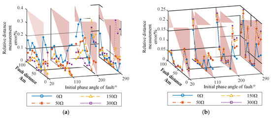

Figure 10.
Impact of fault initial phase angle and fault resistance on fault location accuracy: (a) single-phase-to-ground fault, (b) double-phase-to-ground fault, (c) three-phase fault and (d) phase-to-phase fault.
- Impact of Load Current
This section investigates the impact of load current, which is simulated by adjusting the phase angle difference between the two terminal power supplies. Figure 11 presents the location results under these varying load conditions for different fault types and resistances. The results demonstrate that the relative location error is consistently maintained below 0.4%, confirming the algorithm’s high accuracy and robustness against load current fluctuations.
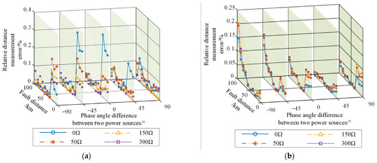

Figure 11.
Impact of load current and fault resistance on fault location accuracy: (a) single-phase-to-ground fault, (b) double-phase-to-ground fault, (c) three-phase fault and (d) phase-to-phase fault.
In conclusion, the algorithm proposed in this paper demonstrates exceptional robustness and high accuracy. The relative location error is consistently maintained below 0.4% across a wide range of operational and fault conditions, including variations in fault location, fault type, fault resistance, initial phase angle, and load current. This performance underscores its potential for reliable application in practical power systems.
5.2.2. Impact of Training Sample Size
To evaluate the algorithm’s performance dependency on the training data volume, the network was trained using varying sample sizes. Figure 12 plots both the average and maximum relative location errors as a function of the sample size. Notably, the algorithm achieves high location accuracy even when the training set is limited to just 50 samples. This result underscores a key advantage of the proposed method: its ability to establish a high-performance fault location model with only a small amount of historical fault data, demonstrating its high data efficiency. The 50-sample subset was selected to maintain the distribution of fault types and fault resistances present in the full dataset, rather than being randomly sampled. While the performance variance across different random subsets was not evaluated, the subset effectively represents the full dataset and validates the method’s data efficiency.

Figure 12.
Impact of training sample size on fault location accuracy.
5.2.3. Performance Comparison with Existing Methods
To further demonstrate the advantages of the proposed algorithm, Table 2 presents a comprehensive performance comparison between the proposed method and the fault location algorithms reported in [8,9,10]. As shown in the table, the proposed algorithm is applicable under scenarios involving unsynchronized data, inaccurate line parameters, different line models, and multi-segment hybrid lines. Moreover, it can directly locate the fault point without identifying the faulted section, exhibiting superior performance compared to the fault location methods in the cited literature.
Table 2.
Performance Comparison of Fault Location Algorithms.
6. Conclusions
This paper proposes a novel fault location algorithm based on data synchronization and a PINN. The methodology begins by employing a data synchronization algorithm to eliminate phase unsynchronization. Subsequently, a fault location function is derived from a distributed-parameter model of the hybrid line. This function facilitates the construction of physics-informed input features, enabling the BP neural network to learn the nonlinear mapping to the fault location with high accuracy.
The proposed algorithm demonstrates several significant advantages. By computationally correcting for phase unsynchronization before performing fault location and by operating independently of line parameters, it exhibits strong robustness against both parameter inaccuracies and unsynchronized measurement data. Extensive simulation results further confirm that the algorithm achieves high location accuracy, with minimal sensitivity to variations in fault type, fault location, fault resistance, fault inception angle, and load current. In addition, by synergistically integrating model-based physical laws with a data-driven approach, the method attains high data efficiency, maintaining excellent performance even when only a limited set of historical fault data is available, which makes it highly suitable for practical applications in power grids.
In addition, due to the small network size (single hidden layer with 10 neurons) and limited training data (up to 304 samples), the offline training of the proposed method is extremely fast, typically less than one second on a standard CPU. Online inference for a single fault instance only requires a few milliseconds, demonstrating that the method readily satisfies real-time requirements for post-fault analysis in control centers.
Moreover, the proposed framework is flexible and can accommodate additional input features in future work; however, increasing input dimensions may require adjustments in network structure to maintain performance, highlighting a trade-off between complexity and accuracy.
For the deployment of a new transmission line, a line-specific fault dataset reflecting the line’s configuration and operating conditions must be generated. The neural network is then trained following the workflow shown in Figure 4 to ensure that the model accurately captures the electrical characteristics of the new line.
The proposed approach is simple, generally applicable to any hybrid line configuration, and allows efficient retraining of neural networks with minimal data. Future work will focus on further improving model generalization.
Author Contributions
Conceptualization, G.Y. and X.C.; methodology, G.Y., G.X., R.J., Y.J., X.C., L.S., Y.L. and Y.G.; software, L.S.; validation, L.S. and Y.L.; investigation, G.Y.; resources, G.Y., G.X., R.J. and Y.J.; data curation, Y.L.; writing—original draft, X.C., L.S., Y.L. and Y.G.; visualization, Y.G.; supervision, X.C.; project administration, X.C.; funding acquisition, G.Y., G.X., R.J., Y.J. All authors have read and agreed to the published version of the manuscript.
Funding
This work was supported in part by State Grid Hebei Electric Power Co., Ltd. under Science and Technology Project No. Kj2023-051 for the project “Research on Parameter Identification and Fault Location Methods for AC Transmission Lines Based on Artificial Intelligence Algorithms”.
Data Availability Statement
The data presented in this study are available on request from the corresponding author due to safety concerns regarding the detailed grid operational parameters and restrictions imposed by the licensing agreement with our industrial partner.
Conflicts of Interest
Author Guangjie Yang, Guojun Xu, Ruijing Jiang, and Yanfeng Jiang were employed by the State Grid Handan Electric Power Supply Company. This study received funding from State Grid Hebei Electric Power Co., Ltd. under Science and Technology Project No. 5204HD230003. The funder was involved in the study design, methodology development, investigation, resource provision, and funding acquisition. All data analysis, interpretation of results, and manuscript writing were performed independently by the authors and were not subject to any undue influence from the funder. The authors declare no other competing financial or non-financial interests.
References
- Dobakhshari, A.S. Wide-area fault location of transmission lines by hybrid synchronized/unsynchronized voltage measurements. IEEE Trans. Smart Grid 2018, 9, 1869–1877. [Google Scholar] [CrossRef]
- Bukvisova, Z.; Orsagova, J.; Topolanek, D.; Toman, P. Two-terminal algorithm analysis for unsymmetrical fault location on 110 kV lines. Energies 2019, 12, 1193. [Google Scholar] [CrossRef]
- Kalita, K.; Anand, S.; Parida, S.K. A closed form solution for line parameter-less fault location with unsynchronized measurements. IEEE Trans. Power Del. 2022, 37, 1997–2006. [Google Scholar] [CrossRef]
- Lu, D.; Liu, Y.; Chen, S.; Wang, B.; Lu, D. An improved noniterative parameter-free fault location method on untransposed transmission lines using multi-section models. IEEE Trans. Power Del. 2022, 37, 1356–1369. [Google Scholar] [CrossRef]
- Livani, H.; Evrenosoglu, C.Y. A machine learning and wavelet-based fault location method for hybrid transmission lines. IEEE Trans. Smart Grid 2014, 5, 10. [Google Scholar] [CrossRef]
- Deng, F.; Zeng, X.; Tang, X.; Li, Z.; Zu, Y.; Mei, L. Travelling-wave-based fault location algorithm for hybrid transmission lines using three-dimensional absolute grey incidence degree. Int. J. Electr. Power Energy Syst. 2020, 114, 105306. [Google Scholar] [CrossRef]
- Huo, W.; Qu, Z.; Ao, Z.; Zhang, Y.; Zhao, E.; Zhang, C.; Jiang, H. Fault location of cable hybrid transmission lines based on energy attenuation characteristics of traveling waves. Sci. Rep. 2022, 12, 22448. [Google Scholar] [CrossRef]
- Liu, C.-W.; Lin, T.-C.; Yu, C.-S.; Yang, J.Z. A fault location technique for two-terminal multisection compound transmission lines using synchronized phasor measurements. IEEE Trans. Smart Grid 2012, 3, 113–121. [Google Scholar] [CrossRef]
- Li, B.-W.; Dong, X.-T.; Wang, L.; Wen, M.-H.; Su, Y.-X. Two-terminal fault location scheme based on distributed parameters of cable-overhead hybrid transmission line. In Proceedings of the 8th Renewable Power Generation Conference (RPG 2019), Shanghai, China, 24–25 October 2019; pp. 1–5. [Google Scholar] [CrossRef]
- Hashemian, S.M.; Hashemian, S.N.; Gholipour, M. Unsynchronized parameterfree fault location scheme for hybrid transmission line. Electr. Power Syst. Res. 2021, 192, 106982. [Google Scholar] [CrossRef]
- Lin, T.-C.; Lin, P.-Y.; Liu, C.-W. An algorithm for locating faults in three-terminal multisection nonhomogeneous transmission lines using synchrophasor measurements. IEEE Trans. Smart Grid 2014, 5, 38–50. [Google Scholar] [CrossRef]
- Lee, Y.-J.; Chao, C.-H.; Lin, T.-C.; Liu, C.-W. A synchrophasor-based fault location method for three-terminal hybrid transmission lines with one off-service line branch. IEEE Trans. Power Del. 2018, 33, 3249–3251. [Google Scholar] [CrossRef]
- Gaur, V.K.; Bhalja, B.R.; Kezunovic, M. Novel fault distance estimation method for three-terminal transmission line. IEEE Trans. Power Del. 2021, 36, 406–417. [Google Scholar] [CrossRef]
- Lak, P.Y.; Ha, K.-M.; Nam, S.-R. A Fault Location Algorithm for Multi-Section Combined Transmission Lines Considering Unsynchronized Sampling. Energies 2024, 17, 703. [Google Scholar] [CrossRef]
- Ngo, Q.-H.; Nguyen, B.L.H.; Vu, T.V.; Zhang, J.; Ngo, T. Physics-informed graphical neural network for power system state estimation. Appl. Energy 2024, 358, 122602. [Google Scholar] [CrossRef]
- Yang, C.; Wu, S.; Liu, T.; He, Y.; Wang, J.; Shi, D. Efficient generation of power system topology diagrams based on Graph Neural Network. Eng. Appl. Artif. Intell. 2025, 149, 110462. [Google Scholar] [CrossRef]
- Békési, G.; Barancsuk, L.; Hartmann, B. Deep neural network based distribution system state estimation using hyperparameter optimization. Results Eng. 2024, 24, 102908. [Google Scholar] [CrossRef]
- de Alencar, G.T.; dos Santos, R.C.; Neves, A. A fault recognition method for transmission systems based on independent component analysis and convolutional neural networks. Electr. Power Syst. Res. 2024, 229, 110105. [Google Scholar] [CrossRef]
- Li, W.; Deka, D.; Chertkov, M.; Wang, M. Real-time faulted line localization and PMU placement in power systems through convolutional neural networks. IEEE Trans. Power Syst. 2019, 34, 4640–4651. [Google Scholar] [CrossRef]
- Luo, G.; Tan, Y.; Li, M.; Cheng, M.; Liu, Y.; He, J. Stacked auto-encoder-based fault location in distribution network. IEEE Access 2020, 8, 28043–28053. [Google Scholar] [CrossRef]
- Wang, X.; Zhou, P.; Peng, X.; Wu, Z.; Yuan, H. Fault location of transmission line based on CNN-LSTM double-ended combined model. Energy Rep. 2022, 8, 781–791. [Google Scholar] [CrossRef]
- Su, C.; Yang, Q.; Wu, X.; Lai, C.S.; Lai, L.L. A two-terminal fault location fusion model of transmission line based on CNN-multi-head-LSTM with an attention module. Energies 2023, 16, 1827. [Google Scholar] [CrossRef]
- Raissi, M.; Perdikaris, P.; Karniadakis, G.E. Physics-informed neural networks: A deep learning framework for solving forward and inverse problems involving nonlinear partial differential equations. J. Comput. Phys. 2019, 378, 686–707. [Google Scholar] [CrossRef]
- Misyris, G.S.; Venzke, A.; Chatzivasileiadis, S. Physics-informed neural networks for power systems. In Proceedings of the IEEE Power Energy Society General Meeting (PESGM), Montreal, QC, Canada, 2–6 August 2020; pp. 1–5. [Google Scholar] [CrossRef]
- Bento, M.E.C. Load margin assessment of power systems using physics-informed neural network with optimized parameters. Energies 2024, 17, 1562. [Google Scholar] [CrossRef]
- Zeng, J.; Li, X.; Dai, H.; Zhang, L.; Wang, W.; Zhang, Z.; Kong, S.; Xu, L. A Residual Physics-Informed Neural Network Approach for Identifying Dynamic Parameters in Swing Equation-Based Power Systems. Energies 2025, 18, 2888. [Google Scholar] [CrossRef]


Disclaimer/Publisher’s Note: The statements, opinions and data contained in all publications are solely those of the individual author(s) and contributor(s) and not of MDPI and/or the editor(s). MDPI and/or the editor(s) disclaim responsibility for any injury to people or property resulting from any ideas, methods, instructions or products referred to in the content. |
© 2025 by the authors. Licensee MDPI, Basel, Switzerland. This article is an open access article distributed under the terms and conditions of the Creative Commons Attribution (CC BY) license (https://creativecommons.org/licenses/by/4.0/).