Article

Collaborative Estimation of Lithium Battery State of Charge Based on the BiLSTM-AUKF Fusion Model

by
Rui Wang
1,2,3,
Lele Liu
1,
Honghou Zhang
3,
Qifeng Qian
3,
Lingchao Xiao
3,
Qiansheng Qiu
3,
Chao Tan
2 and
Fujian Yang
4,*
1
School of Wangzheng Microelectronics, Changzhou University, Changzhou 213164, China
2
School of Electrical and Information Engineering, Tianjin University, Tianjin 300072, China
3
Zhejiang Sunoren Solar Technology Co., Ltd., Haining 314400, China
4
School of Urban Construction, Changzhou University, Changzhou 213164, China
*
Author to whom correspondence should be addressed.
Energies 2025, 18(21), 5624; https://doi.org/10.3390/en18215624
Submission received: 15 September 2025 / Revised: 18 October 2025 / Accepted: 23 October 2025 / Published: 26 October 2025

Abstract

To address the issue of decreased accuracy in lithium battery state of charge (SOC) estimation caused by parameter mismatches, modeling error accumulation, and sensitivity to noise, this paper proposes a collaborative estimation method. The proposed method combines a Bayesian optimization (BO)-tuned dual-input bidirectional long short-term memory network (BiLSTM) with an adaptive unscented Kalman filter (AUKF) based on the Sage–Husa adaptive strategy. First, a dual-input BiLSTM network is constructed using a multi-layer cascaded BiLSTM to extract time-dependent features. This network fuses both temporal and static features to perform an initial SOC prediction, while BO is employed to adaptively optimize the network’s hyperparameters. Second, the BiLSTM prediction outputs and the physical model are incorporated into the AUKF framework to achieve real-time iterative SOC estimation. Multi-scenario experiments conducted on the University of Maryland CALCE battery dataset demonstrated that the proposed method achieved a mean absolute error (MAE) below 0.6% and a root mean square error (RMSE) less than 0.8%. This method effectively enhances the robustness and noise immunity of SOC estimation in dynamic scenarios, providing a high-precision state estimation solution for battery management systems.

1. Introduction

Accurate estimation of SOC in lithium-ion batteries serves as a core technology for battery management systems to achieve energy optimization, lifespan prediction, and safety control [1]. However, the SOC of lithium batteries cannot be directly measured. Moreover, the complex electrochemical characteristics within batteries and the highly nonlinear relationships under dynamic operating conditions result in challenges in SOC estimation, such as multi-timescale coupling, time-varying parameters, and noise interference [2]. Existing methods are primarily categorized into three approaches: direct measurement, model-driven, and data-driven techniques [3]. Direct measurement methods are exemplified by the open-circuit voltage (OCV) method and the ampere-hour (Ah) integration method. The OCV method directly maps SOC through the OCV-SOC calibration curve, but it requires prolonged battery rest periods, making it impractical for real-time applications [4,5]. The Ah integration method calculates SOC by accumulating charge and discharge currents. However, it is susceptible to initial SOC errors and current sensor noise [6].
Model-based approaches utilize physical models combined with filtering algorithms to achieve SOC estimation, such as the Kalman filter (KF) and particle filters [7,8,9,10,11]. Commonly adopted models include the equivalent circuit model (ECM) or electrochemical models [12]. Although electrochemical models can fundamentally reveal complex internal reactions through physical and chemical principles, their practical application remains limited due to inherent complexity and difficulties in accurate parameter identification [13]. Among ECMs, the Thevenin model is widely adopted for its computational simplicity and ability to reflect internal mechanisms to a certain extent [14,15,16]. However, the model-based approach emphasizes the accuracy of the model, and the variation of model parameters in different environments and states makes it challenging to maintain the accuracy of SOC estimation.
Data-driven approaches leverage machine learning and deep learning algorithms to establish a mapping relationship between SOC and battery measurement data [17,18,19,20,21,22]. These methods yield accurate estimation results and demonstrate strong capabilities in handling nonlinear relationships [23]. However, they suffer from notable drawbacks, including a lack of explicit physical interpretability, time-consuming training processes, and performances that heavily depend on data quality [24]. In practical applications, ensuring the quality of collected data remains challenging due to sensor inaccuracies and external environmental interference.
Therefore, combining the strengths of different methods for joint estimation has become a research focus [25,26,27]. Yang et al. [28] employed an LSTM network to estimate battery SOC, followed by a UKF to reduce estimation errors. Xu et al. [29] utilized a broad learning system to model battery voltage characteristics and subsequently applied UKF for SOC estimation. Tian et al. [30], based on a first-order RC equivalent circuit model and an extended Kalman filter (EKF), decomposed the battery terminal voltage to extract internal physical information, which was then fed into an LSTM for training. This approach enriched the neural network’s feature inputs and enhanced SOC estimation performance. Takyi-Aninakwa et al. [31] adopted an adaptive singular value decomposition-based unscented Kalman filter combined with an LSTM extended-input model. This framework reliably and accurately estimates SOC under diverse operating conditions by incorporating battery domain-specific parameters. Chen et al. [32] leveraged LSTM to establish a coarse estimation model linking input voltage, current, operating temperature, and state of health to SOC. An adaptive H-infinity Filter was then applied to suppress output fluctuations and improve estimation accuracy. Similarly, Wang et al. [33] proposed a closed-loop framework based on a deep convolutional neural network. To enhance the filter’s robustness against non-Gaussian noise, a maximum correntropy square-root cubature Kalman filter was applied to smooth the network’s SOC output. For further computational efficiency and stability, the literature [34] introduced a novel SOC estimation method using a simplified gated recurrent unit (GRU) structure integrated with an adaptive Kalman filter (AKF). Initial filter parameters were set based on the evolution of the Kalman gain to achieve superior SOC convergence. Additionally, Wei et al. [35] combined a nonlinear autoregressive model with exogenous inputs (NARX) with AKF, while [36] integrated Ada-CNN-GRU with KF. Consequently, compared to purely model-based or data-driven approaches, these hybrid methods exhibit enhanced observability, reduced output fluctuations, and superior SOC estimation performance.
However, these hybrid strategies still face multiple challenges in practical deployment. Most methods are not only highly sensitive to parameter tuning but also prone to error accumulation over prolonged operation. Moreover, their filters often rely on static noise assumptions, which struggle to adapt to the dynamic changes in real-world environments. The widespread dependence on manual parameterization not only reduces practicality but also introduces the risk of subjective errors. Furthermore, co-estimation frameworks are often plagued by high computational complexity and inadequate handling of model–data mismatches—a shortcoming that is particularly exacerbated under varying temperatures and aging conditions. As a result, the stability of existing algorithms is compromised in practical applications due to their complexity and parameter sensitivity. The need for frequent manual adjustments and retraining in dynamic environments further diminishes operational efficiency and may introduce additional errors due to human intervention, leading to performance degradation.
To address these challenges, this study proposes a synergistic estimation framework that integrates a BO-tuned dual-input BiLSTM network with an AUKF. The methodology implements a three-phase optimization: (1) A BO-optimized BiLSTM fuses temporal and static features for high-precision initial SOC prediction; (2) the particle swarm optimization (PSO) identifies ECM parameters to establish physical voltage-SOC constraints; (3) BiLSTM outputs and ECM are embedded within the UKF framework, where the Sage-Husa strategy dynamically calibrates noise statistics online to suppress error accumulation. Experimental validation across various temperatures and operating conditions confirmed the algorithm’s superior estimation accuracy and enhanced robustness.

2. Problem Model

The internal circuit configurations of different energy storage systems (ESS) vary significantly, posing challenges in accurately obtaining internal circuit details during SOC estimation. To address this, it is necessary to develop charge–discharge models that establish a mathematical relationship between SOC and circuit parameters. In ECMs, while the first-order RC model has a simple structure, it often fails to accurately capture dynamic characteristics such as the slow diffusion processes within the battery. In contrast, higher-order RC network models can slightly improve accuracy but require the introduction of numerous unknown parameters, leading to increased model identification complexity. Considering the optimal balance between accuracy and complexity, we adopted the widely used second-order RC equivalent circuit model, structure shown in Figure 1. The second-order RC network effectively represents key dynamic characteristics such as electrochemical polarization and concentration polarization. Furthermore, the parameters of this model can be conveniently identified experimentally, ensuring both feasibility for real-time battery management system (BMS) estimation and reliability.
In this model, the first resistor-capacitor (RC) network is employed to characterize the electrochemical polarization induced by the battery’s charge transfer process, while the second RC network models the concentration polarization arising from lithium-ion diffusion. The polarization voltages U1 and U2 corresponding to these two RC networks satisfy the following system of differential equations, i.e.,
{ d U 1 d t = U 1 R 1 C 1 + I C 1 d U 2 d t = U 2 R 2 C 2 + I C 2
Based on Figure 1, the relationship between the voltages in the equivalent circuit can be expressed as
U T = U OC ( SOC ) I R 0 U 1 U 2
where the UT is the terminal voltage, the UOC denotes the open-circuit voltage, and the relationship between UOC and SOC can be determined through low-rate battery’s charge- discharge experiments, as detailed in Section 7.2.
Using the Ah integration method, the SOC variation is calculated by integrating the battery’s charging or discharging current during operation, as given by
SOC ( t ) = SOC 0 1 C nom 0 t η I ( τ ) d τ
where SOC0 represents the initial SOC, Cnom denotes the battery’s available capacity, I(t) is the instantaneous current, and η stands for the Coulombic efficiency (η ≤ 1 during charging since part of the electrical energy is lost as heat dissipation, while typically set to η = 1 during discharging).
Discretizing Equations (1)–(3) into the discrete equivalent circuit model for SOC estimation, we obtain the corresponding discrete-time model as
{ SOC ( k ) = SOC ( k 1 ) η × Δ t C nom I ( k 1 ) U T ( k ) = U OC ( SOC ( k ) ) R 0 × I ( k ) U 1 ( k ) U 2 ( k ) U 1 ( k ) = e Δ t R 1 C 1 U 1 ( k 1 ) + R 1 ( 1 e Δ t R 1 C 1 ) I ( k 1 ) U 2 ( k ) = e Δ t R 2 C 2 U 2 ( k 1 ) + R 2 ( 1 e Δ t R 2 C 2 ) I ( k 1 )
Let the model parameter vector of the equivalent circuit in Equation (4) be denoted as V = [R0, R1, R2, C1, C2]T. By minimizing the mean square error between the simulated terminal voltage UT(k) and the corresponding measured counterpart Umeas(k), a cost function with respect to V is formulated as
V = min V { 1 N k = 1 N [ U T ( k ) U meas ( k ) ] 2 }
This cost function exhibits strong nonlinearity and involves high-dimensional unknown parameters. To prevent the solution process from converging to local minima, this study employs the PSO algorithm for parameter identification, as detailed in Section 4. Following the acquisition of equivalent circuit model parameters, SOC estimation is equivalent to a prediction problem. While such problems can be addressed using Kalman filter variants or LSTM networks, Kalman-type algorithms demonstrate high sensitivity to model inaccuracies, and LSTM suffers from the absence of physics-based constraints. Consequently, this work proposes a hybrid framework integrating BiLSTM with UKF. BiLSTM compensates for UKF’s model uncertainties, while BO and Sage–Husa adaptive filtering jointly regulate the hyperparameters of the BiLSTM network and the noise statistics of the UKF algorithm.

3. Collaborative Estimation of Battery SOC Based on BiLSTM-AUKF Fusion Model

To achieve high-accuracy lithium battery SOC estimation, a dual-input BiLSTM network architecture is introduced in this paper. This design employs multi-stage cascaded BiLSTM layers to extract time-dependent features, while fusing temporal characteristics with static features for preliminary SOC prediction, which is further enhanced by BO for adaptive hyperparameter tuning. Subsequently, an ECM framework is established, in which PSO algorithms identify model parameters, constructing a nonlinear mapping between terminal voltage and SOC. The outputs from both BiLSTM predictions and this physical model are then integrated into a UKF framework to enable real-time iterative SOC estimation. Furthermore, the UKF implementation incorporates a Sage-Husa adaptive strategy to dynamically calibrate state and observation noise statistics during operation. This dual approach effectively mitigates cumulative model errors while significantly enhancing noise robustness. Figure 2 depicts the comprehensive flowchart for the BiLSTM-AUKF fusion model approach to power lithium-ion battery SOC estimation.

4. PSO-Based Parameter Identification for Battery ECM

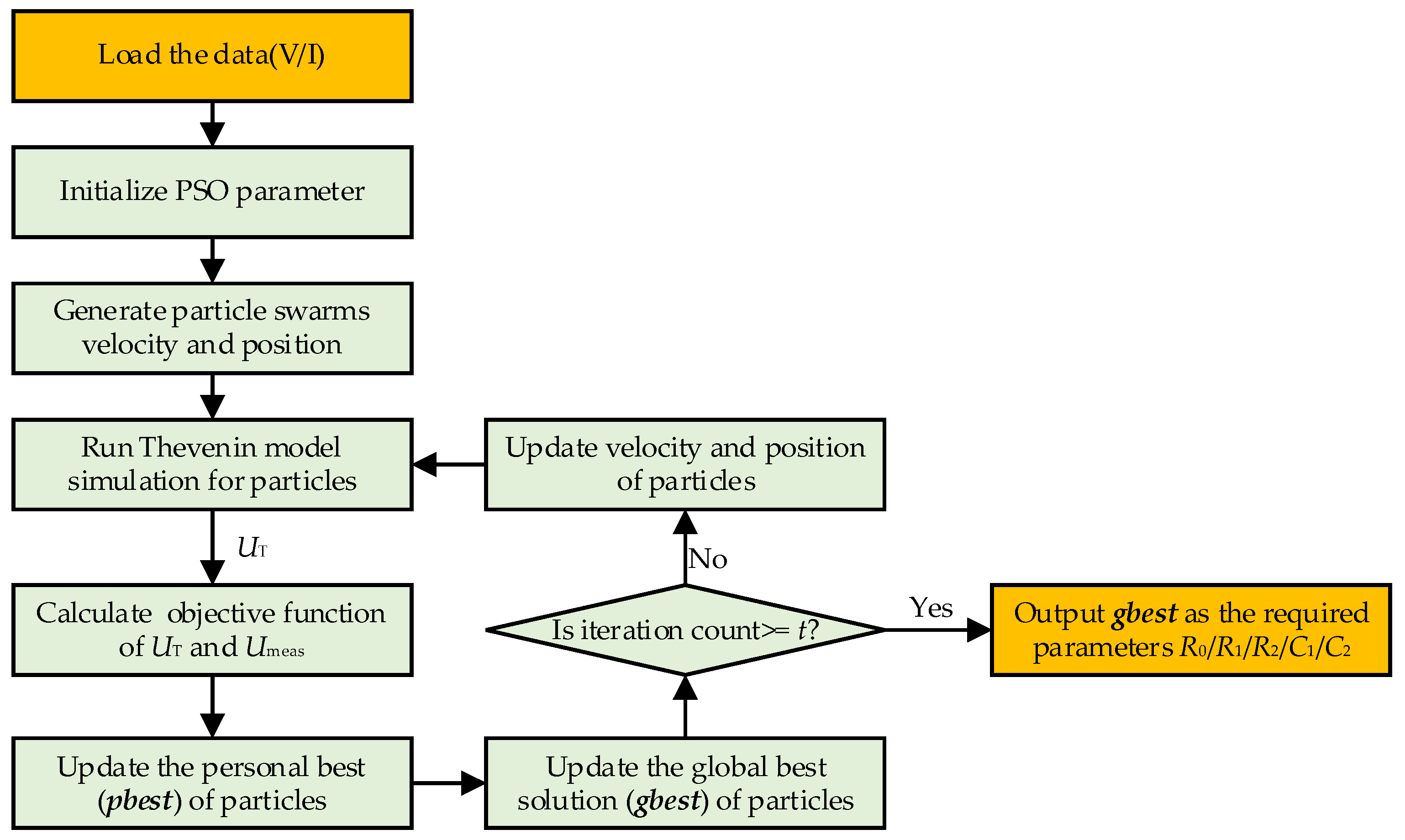
Rooted in swarm intelligence theory, the PSO emulates collective foraging mechanisms in bird flocks. Leveraging its powerful global exploration capabilities, PSO effectively enhances the identification accuracy for multiparameter nonlinear systems. This study employs the PSO algorithm to identify the parameter vector V = [R0, R1, R2, C1, C2]T of the equivalent circuit model, with the procedure illustrated in Figure 3. Algorithmically, each particle represents a five-dimensional parameter vector, and its trajectory characterizes the dynamic optimization process.
Within the PSO algorithm framework, given a population size of n, the position vector Pi = [xi,1, xi,2, xi,3, xi,4, xi,5]T and velocity vector Si = [si,1, si,2, si,3, si,4, si,5]T are defined for each particle i in the five-dimensional parameter space. Each dimension of Pi corresponds to an element of the equivalent circuit parameter vector V under identification, while Si characterizes the search direction and step size of the parameter vector. The RMSE between measured terminal voltage Umeas and model output voltage UT serves as the fitness function. Through iterative updates of particle positions and velocities, the RMSE value is minimized, driving Pi to progressively approach the true physical parameters. Each particle’s position and velocity are dynamically adjusted according to its personal best (pbesti) and the global best (gbest). Equation (6) defines pbestit as the position corresponding to the minimum fitness value (RMSE) discovered by particle i at iteration t, and gbestt is the position of the minimum fitness value among all particles’ personal bests.
{ p b e s t i t = argmin T { 1 , 2 , , t } RMSE ( P i T ) g b e s t t = argmin i { 1 , 2 , , n } RMSE ( p b e s t i t )
The state update expressions for the velocity and position of particle i at iteration t are given by
{ S i t + 1 = ω S i t + α 1 r 1 ( p b e s t i t S i t ) + α 2 r 2 ( g b e s t t S i t ) P i t + 1 = P i t + S i t + 1
Here, the ω denotes the inertia weight, the α1 and the α2 are learning factors, the r1 and the r2 represent uniformly distributed random numbers within [0, 1]. Through iterative application of Equation (7), the algorithm computes the updated fitness value (RMSE) for each particle. If the new RMSE is lower than the previous value, the particle updates its state; otherwise, the original state is retained. After all particles’ fitness values are updated, the system re-evaluates the global best solution (gbest). If the fitness value of gbest improves, it is updated; otherwise, the current solution is maintained. The optimization terminates when the maximum iteration count t is reached. The globally optimal parameter set gbest is then assigned to the model parameter vector V for subsequent battery SOC estimation. By integrating both the personal best (pbesti) and global best (gbest) solutions in a dual-level selection mechanism, the optimization process ensures the continuous preservation of historically optimal solutions.

5. BO-BiLSTM-Based SOC Prediction

5.1. LSTM Cell Structure

As a variant of recurrent neural networks (RNNs), the LSTM fundamentally resolves the vanishing and exploding gradient issues in traditional RNNs during long sequence processing. Its core innovation lies in the integration of a persistent cell state and gated control mechanisms. The cell state enables continuous information flow across time steps, while the forget, input, and output gates dynamically regulate information retention, updating, and output. This architecture allows LSTM to capture long-term dependencies in sequential data, delivering significant advantages for battery SOC estimation that requires extended temporal dependency modeling.
The computational flow of an LSTM network cell at time step k proceeds as follows: The forget gate determines the proportion of information discarded from the current cell state. It generates output fk based on the current input uk and the previous hidden state hk−1.
f k = σ ( W f [ h k 1 , u k ] + b f )
The input gate regulates which information from uk and hk−1 is stored in the cell state Ck. Input gate output ik is generated by using the sigmoid activation function, and the new candidate value C ~ k is generated using the tanh activation function for subsequent cell state updates.
{ i k = σ ( W i [ h k 1 , u k ] + b i ) C ˜ k = tanh ( W C [ h k 1 , u k ] + b C )
Cell state propagation maintains information continuity across extended time intervals. The current cell state Ck is updated by combining the prior state Ck−1 with new input data, i.e.,
C k = f k C k 1 + i k C ˜ k
The output gate controls which information from the updated cell state Ck is emitted as the current hidden state hk. Generate the output Ok of the output gate by using uk and hk−1, and then combine it with the current moment’s cell state Ck to generate hk, which is output to the next layer or the next time step.
{ O k = σ ( W O [ h k 1 , u k ] + b O ) h k = O k tanh ( C k )
where Wf, Wi, WO, WC are weight matrices, bf, bi, bO, bC are bias vectors. The σ(·) is the sigmoid activation function (which compresses values to [0, 1]), with outputs approaching 1 indicating high information retention. The tanh(·) is the tanh activation function (which outputs to [−1, 1]), encoding bipolar information.
This describes the LSTM network’s process of updating the cell state and output (hidden state) through sequential inputs. It filters out irrelevant information while propagating critical features, thereby endowing the model with robust long-term memory retention. This architecture effectively overcomes long-distance dependency problems, enabling efficient prediction of time-series data.

5.2. BiLSTM Network

This study addresses the unidirectional limitation of LSTM networks in time-series learning, which neglects bidirectional relationships between information units and underutilizes features across the entire temporal sequence. By incorporating reverse-sequence correlations alongside forward dependencies, we construct a BiLSTM neural network model. The BiLSTM architecture integrates two independent LSTM networks with symmetric cell structures, identical inputs, and opposing information flow directions. This design enables simultaneous extraction of intrinsic relationships between current sequence information, historical context, and future states. Hidden-layer neurons store features from both directional sequences, significantly enhancing prediction capability and data utilization efficiency. Figure 4 illustrates the information propagation mechanism within BiLSTM neural units at each time step.
Take the output hkl of the lth (l = 1, 2, …, L) layer at time instant k in the hidden layer as an example.
{ h k = N E ( u k , h k 1 ) h k = N E ( u k , h k + 1 ) h k l = h k h k
Here, NE(∙) denotes the LSTM cell’s update computation process generating outputs based on timestep inputs and the previous hidden state, with detailed equations provided in (8)–(11). The terms h k and h k represent forward-updated and backward-updated hidden states, respectively. ⊕ is the vector concatenation operator. The fused hidden state hkl∈R2Cunits, where Cunits denotes the dimensionality of a single LSTM layer’s hidden state (the number of hidden layer units). By integrating outputs from both directional hidden layers, the model captures richer informative features, significantly enhancing its learning capacity and robustness.
This paper proposes a dual-input BiLSTM architecture comprising two core modules: sequential feature learning and feature fusion, as depicted in Figure 5. In the sequential feature learning module, the sequence processing branch receives time-series input data. Specifically, sequential battery data Dseq = [d1, d2, …, dT] where dk = [Uk, Ik, Tempk]T. Through multiple cascaded BiLSTM layers, intrinsic temporal dependencies are extracted. For the initial L-1 layers, outputs preserve complete sequence information as Hl = [h1l, h2l, …, hTl]. The final BiLSTM layer outputs only the last timestep’s hidden state hseqL to capture global temporal evolution characteristics. In the feature fusion module, the static feature branch receives non-sequential inputs at the current timestep. These features are encoded via a fully connected layer to produce hs, which is projected into a feature space dimensionally compatible with the sequence branch’s output. The static branch output is given by
h s = ReLU ( W s x s + b s )
The static feature input in this study is defined as a scalar xs, derived from Equation (3) as a rough SOC estimate based on Coulomb counting. This input injects physically grounded prior knowledge into the model, providing initialization for the state evolution dynamics. Subsequently, the sequence branch’s final output hseqL and the static feature branch’s output hs are concatenated into a fused vector hfusion = [hseqL; hs]. This operation synergistically integrates historical sequential dynamics from hseqL and current static state information from hs. The fused feature vector then undergoes nonlinear transformation and dimensionality reduction through a multi-layer fully connected network (incorporating ReLU activations and dropout layers), yielding hout. This design enhances nonlinear representation capacity while mitigating overfitting risks, thereby strengthening generalization capability. The computation of hout is given by
h out = Dropout [ ReLU ( W fusion h fusion + b fusion ) , p ]
Therefore, the predicted SOC values Y ˜ i generated by forward propagation of Dseq through the dual-input BiLSTM model are obtained as
Y ˜ i = W out h out + b out
Here, DseqRC×T denotes the input sequence matrix, hseqL∈ R2Cunit represents the final BiLSTM hidden state. The parameter C signifies the input feature dimension, while T corresponds to the time step length. The Uk, Ik, and Tempk represent the voltage, current, and temperature measurements at time step k in the battery time-series data. Thus, the feature dimension C = 3. In Equations (13)–(15), Ws, Wfusion, and Wout are weight matrices, and bs, bfusion, and bout are bias vectors. The ReLU(·) serves as the activation function, and Dropout(·) as the random masking mechanism, and p as the dropout probability.
During model training, the mean squared error (MSE) serves as the regression loss function to quantify the discrepancy between the BiLSTM-predicted SOC values Y ˜ i and the reference SOC values Yi. Given a batch size B, the MSE is formally defined as
ε = 1 B i = 1 B ( Y i Y ˜ i ) 2
Let the set of learnable parameters be denoted as φ = {φBiLSTM, φFC}, where gradients of the loss function with respect to these parameters are computed layer-wise via backpropagation:
ε = ε Y ˜ Y ˜ φ
Gradients for fully connected layers are computed layer-wise via the chain rule, while the BiLSTM layer employs the Backpropagation Through Time (BPTT) algorithm to calculate gradients accumulated across timesteps, i.e.,
ε φ BiLSTM = k = 1 T ε h seq L h seq L φ BiLSTM
The gradient of the loss function, serving as the error signal, propagates backward through the network topology via the backpropagation algorithm, traversing both fully connected layers and BiLSTM layers. The Adam gradient descent algorithm synchronously updates all learnable parameters across the sequence feature module and the feature fusion module as follows:
φ new = φ η L ε
Here, φFC denotes the parameters of the feature fusion module (including the weights and biases of the static encoding layer, the concatenation layer, and the subsequent fully connected networks), φBiLSTM represents the parameters of the sequence feature module (the weights and biases of BiLSTM layers), and ηL denotes the learning rate.
Through this architecture, end-to-end joint training is performed until model convergence, significantly enhancing the robustness and accuracy of SOC estimation under complex operating conditions and providing a reliable solution for battery state estimation.

5.3. Bayesian Optimization

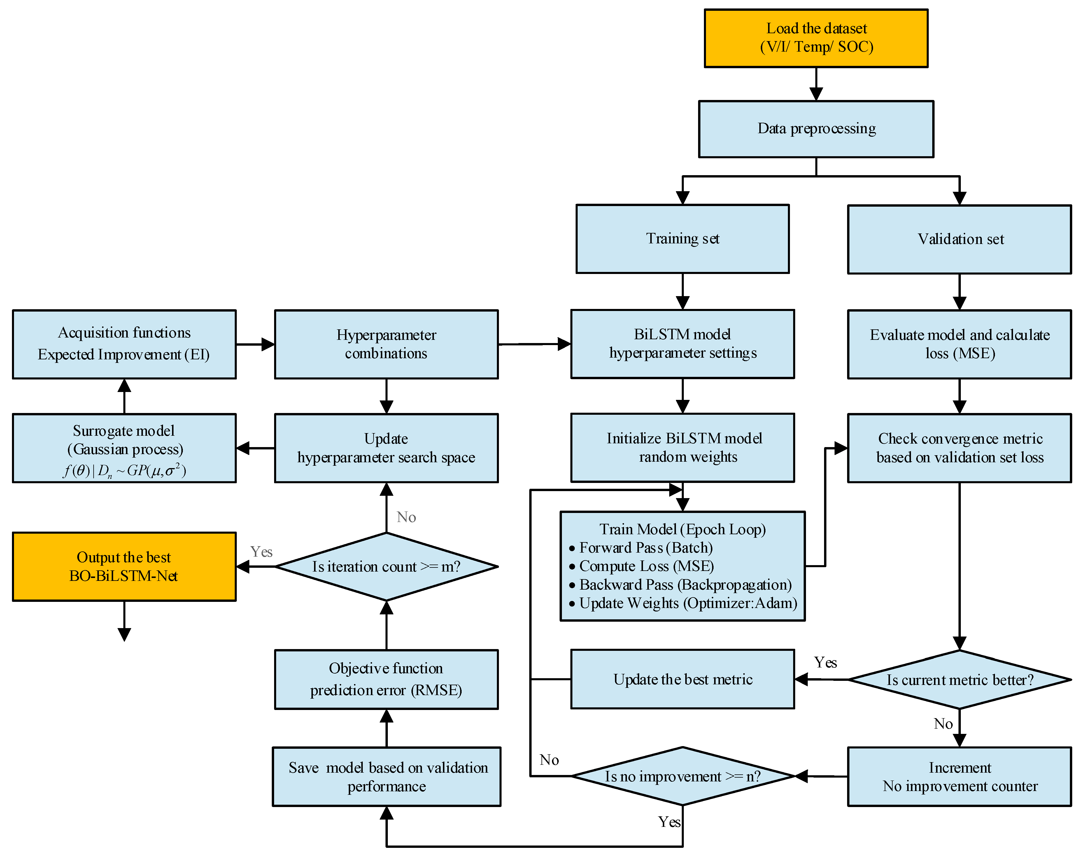
The dual-input BiLSTM network architecture proposed in this study incorporates several critical hyperparameters (e.g., the number of hidden layers, the number of hidden units per layer, dropout rate, the dimensions of the fully connected layer, and the regularization coefficients). To efficiently determine the optimal configuration of these hyperparameters while avoiding laborious and subjective manual tuning, this paper employs BO for automated hyperparameter optimization. The BO algorithm minimizes the RMSE of model predictions on an independent validation set as its objective function, conducting adaptive sampling and evaluation within predefined hyperparameter search spaces.
Let the set of hyperparameters to be optimized be denoted as θΨ, where θ is a vector comprising the number of hidden units, dropout rate, fully connected layer dimensionality, and regularization coefficient. Here, Ψ represents the predefined feasible search space for each hyperparameter. The objective function f(θ) is defined as the RMSE of predictions generated by the BiLSTM model, trained under hyperparameter configuration θ, computed on an independent validation set. This function is minimized via Bayesian Optimization.
θ best = arg min f ( θ ) θ Ψ
The BO algorithm assumes that the objective function f(θ) is governed by a Gaussian Process (GP) prior distribution:
f ( θ ) G ( μ ( θ ) , k ( θ , θ ) )
Here, μ(θ) denotes the mean function, k(θ, θ) is the covariance function (kernel function), which quantifies the correlation between any two points θ and θ within the hyperparameter search space Ψ. Specifically,
k ( θ , θ ) = σ f 2 e ( 1 2 l 2 θ θ 2 )
The kernel function k(θ, θ) quantifies the similarity in the impact of different hyperparameter configurations on model performance. When k(θ, θ) approaches σ f 2 , it indicates that the two hyperparameter configurations exert strongly correlated effects on BiLSTM performance. Conversely, when k(θ, θ) approaches 0, the configurations exhibit nearly independent influences on BiLSTM performance. Here, σ f 2 denotes the signal variance, which controls the magnitude of variation in the objective function and corresponds to potential fluctuations. The l represents the length-scale, which governs the smoothness of the function.
Given that n evaluations have been conducted, the hyperparameter configurations and their corresponding objective function values constitute the observed dataset Dn:
D n = { ( θ i , y i ) } i = 1 n
where yi denotes the observed objective function value (validation set RMSE) obtained from the BiLSTM model under hyperparameter configuration θi. To account for potential stochasticity in the evaluation process, yi is modeled as the true objective function value f(θi) perturbed by Gaussian noise δi:
y i = f ( θ i ) + δ i , δ i ~ ( 0 , σ r 2 )
where σ r 2 denotes the noise variance, which quantifies the magnitude of evaluation errors (e.g., the fluctuations induced by training stochasticity).
Given the observed dataset Dn and GP prior, the posterior distribution of the true objective function f(θ*) at any candidate point θ*Ψ, follows a Gaussian distribution:
f ( θ * ) | D n N ( μ ( θ * ) , σ 2 ( θ * ) )
The mean μ(θ*) and variance σ2(θ*) of the posterior distribution are given by
{ μ ( θ * ) = G T ( A + σ r 2 I ) 1 y σ 2 ( θ * ) = k ( θ * , θ * ) G T ( A + σ r 2 I ) 1 G
where μ(θ*) represents the optimal estimate (predicted value) of f(θ*) given the dataset Dn, while σ2(θ*) quantifies the uncertainty in this estimate. The n × n covariance matrix A has elements Aij = [k(θi,θj)] denoting pairwise covariances between observed points. The vector G = [k(θ*,θ1), …, k(θ*,θn)]T represents covariances between the candidate point θ* and observed points. The vector y = [y1, …, yn]T contains known objective function values, and I denotes the n × n identity matrix.
The GP provides predictions (mean) and uncertainty quantification (variance) for the objective function at unevaluated points θ*. Leveraging the posterior distribution, an acquisition function selects the next evaluation point θnew with the highest potential to improve upon the current best result. This function strategically balances exploration (sampling high-uncertainty regions) and exploitation (sampling near currently optimal regions). This study employs expected improvement (EI) as the acquisition function, denoted βEI(θ*). EI quantifies the expected improvement achievable by evaluating the objective at θ* relative to the current best observed value fn+:
β EI ( θ * ) = E [ ( max ( 0 , f ( θ * ) f n + ) ]
The next evaluation point θnew is selected by maximizing the EI acquisition function, i.e.,
θ new = arg max θ * Ψ   β EI ( θ * )
Train the BiLSTM network using the hyperparameter configuration θnew, compute its RMSE on the validation set (Equation (24)) to obtain ynew. Augment the dataset Dn with this new observation by incorporating (θnew, ynew), and update the Gaussian process model accordingly.
Iterate this process continuously until reaching the predefined maximum evaluation count m. Upon termination, select the optimal hyperparameter configuration θbest from all evaluated points to configure the BiLSTM network for subsequent battery SOC estimation. The Bayesian optimization workflow for the BiLSTM network is illustrated in Figure 6.

6. UKF with Sage-Husa Adaptive Strategy

The final framework feeds the predicted battery SOC estimates from the BO-BiLSTM network into a physics-based AUKF module. The AUKF algorithm further optimizes the SOC estimates to enhance estimation accuracy.
The physics-based AUKF defines the state vector as x = [SOC, U1, U2] according to Equation (4), with a dimension of n = 3. At time step k, it initializes mean weights Wm and covariance weights Wc. These weights aggregate sigma points to compute statistical quantities (mean and covariance) during the prediction and update steps. Here, α and β are scaling parameters for the unscented transform (UT), while λ denotes a composite scaling coefficient.
{ W m [ 0 ] = λ n + λ , W c [ 0 ] = λ n + λ + ( 1 α 2 + β ) W m [ i ] = W c [ i ] = 1 2 ( n + λ ) , i = 1 , , 2 n
Based on the state vector x ^ k 1 and covariance matrix P k 1 at the previous time step, a set of sigma points is generated by using the UT to select 2n + 1 points around x ^ k 1 .
{ ς k 1 0 = x ^ k 1 ς k 1 i = x ^ k 1 + ( n + λ ) P k 1 , i = 1 , , n ς k 1 n + i = x ^ k 1 ( n + λ ) P k 1 , i = 1 , , n
Propagate the sigma points through the state transition function F(∙) to obtain the predicted state mean x ^ k and predicted covariance matrix P k at the current time step. The state equation F(∙) is constructed from the state variables according to Equation (4).
{ x ^ k = i = 0 2 n W m [ i ] F ( ς k 1 i ) P k = i = 0 2 n W c [ i ] [ F ( ς k 1 i ) x ^ k ] [ F ( ς k 1 i ) x ^ k ] T + Q k 1
Based on the state mean x ^ k and covariance matrix P k from the Prediction step, a set of sigma points is generated by using the UT to select 2n + 1 points around x ^ k .
{ ς k 0 = x ^ k ς k i = x ^ k + ( n + λ ) P k , i = 1 , , n ς k n + i = x ^ k ( n + λ ) P k , i = 1 , , n
Propagate the sigma points obtained from the prediction step through the observation equation J(∙) to compute the observation mean vector Z ^ , observation covariance matrix P z z , and cross-covariance matrix P x z . The observation function J(∙) is defined by Equation (2), which models battery terminal voltage.
{ Z ^ = i = 0 2 n W m [ i ] J ( ς k i ) P x z = i = 0 2 n W c [ i ] [ F ( ς k 1 i ) x ^ k ] [ J ( ς k i ) Z ^ ] T P z z = i = 0 2 n W c [ i ] [ J ( ς k i ) Z ^ ] [ J ( ς k i ) Z ^ ] T + R k 1
The update residual ek is computed using the actual measured terminal voltage Umeas and the output value Y ~ from the BiLSTM network.
e k = [ U meas ( k ) U ( k ) ; Y ˜ ( k ) SOC ( k ) ]
The residual ek is utilized to update the predicted state, yielding the updated state estimate mean vector x ^ k and covariance matrix P k , thereby completing the state update and estimation for time step k. Specifically,
{ K k = P x z P z z 1 x ^ k = x ^ k + K k e k P k = P k K k P z z K k T
where Kk is the Kalman gain matrix at time step k.
In UKF, the system process noise covariance matrix Qk and measurement noise covariance matrix Rk must be specified. Incorrect specification of Qk and Rk introduces estimation errors that accumulate over time, leading to rapid error propagation and potential filter divergence. This paper employs the Sage–Husa adaptive strategy to dynamically estimate Qk and Rk, enabling real-time adaptation to noise statistical characteristics and mitigating filter divergence. Based on the maximum likelihood principle, this strategy iteratively estimates noise statistics using filtered values and one-step predictions. After the UKF update (Equation (35)), Qk and Rk are updated as follows:
{ S k = e k e k T i = 0 2 n W c [ i ] [ J ( ς k i ) Z ^ ] [ J ( ς k i ) Z ^ ] T T k = i = 0 2 n W c [ i ] [ F ( ς k 1 i ) x ^ k ] [ F ( ς k 1 i ) x ^ k ] T R k = ( 1 d k ) R k 1 + d k S k Q k = ( 1 d k ) Q k 1 + d k ( K k e k e k T K k T + P k T k )
where dk is the forgetting factor given by dk = 1 c 1 c k + 1 (0 < c < 1), which progressively diminishes the influence of older measurements. As time advances, dk asymptotically approaches 1 − c. By leveraging the Kalman gain to correct discrepancies between predicted and actual observation vectors, the state estimates are continuously iteratively updated to achieve higher-precision battery SOC estimation. The workflow is illustrated in Figure 7.

7. Model Validation and Analysis

7.1. Datasets and Metrics

To systematically validate the feasibility, accuracy, and robustness of the proposed dual-input BiLSTM-AUKF fusion model for SOC estimation in lithium-ion batteries, this study conducted experiments using an A123 LiFePO4 battery with a nominal capacity of 1100 mAh, a nominal voltage of 3.3 V, and an operational voltage window between 2.0 V and 3.6 V. The hardware environment for the experiments was configured with an Intel Core i9-10900KF CPU @ 3.70 GHz, 64 GB RAM (original equipment manufacturer: Intel Corporation; headquartered in Santa Clara, CA, USA), and an NVIDIA GeForce RTX 4060 Ti GPU (NVIDIA Corporation; headquartered in Santa Clara, CA, USA), while the software platform utilized the Windows 11 operating system and MATLAB R2024a.
Initially, low-current charge–discharge cycles were performed to obtain OCV characteristic data, and the PSO algorithm was employed for parameter identification, establishing the foundation for battery modeling in subsequent SOC estimation algorithms. Subsequently, at 20 °C, the SOC estimation accuracies of GRU, LSTM, BiLSTM, BiLSTM-UKF, and the proposed dual-input BiLSTM-AUKF algorithms were compared across three typical driving cycles: dynamic stress test (DST), federal urban driving schedule (FUDS), and highway driving test (US06). By analyzing estimation results and errors, this work quantitatively evaluated the structural advantages of BiLSTM networks and the role of the Sage–Husa adaptive strategy in enhancing UKF performance. Finally, the robustness and generalization capability of the BiLSTM-AUKF algorithm were validated under inaccurate initial SOC settings (initial error) and varying ambient temperatures. First, different initial SOC values (90%, 80%, 70%; true value: 100%) were tested at 20 °C to examine their convergence robustness. Second, the algorithm was operated at 0 °C, 10 °C, and 40 °C to assess its temperature adaptability.
The experimental data originated from the publicly available dataset of the CALCE Battery Group at the University of Maryland [37], which was obtained by simulating real-world electric vehicle driving scenarios. This dataset includes dynamic battery operational data (voltage, current, and temperature) under three typical driving profiles—DST, FUDS, and US06—tested at different environmental temperatures.
This paper employs the maximum error (MaxError), the root mean squared error (RMSE), and the mean absolute error (MAE) as evaluation metrics, which are expressed, respectively, as follows:
{ MaxError = max i = 1 , , n | y i y ^ i | RMSE = 1 n i = 1 n ( y i y ^ i ) 2 MAE = 1 n i = 1 n | y i y ^ i |
where yi and ŷi denote the true value and the predicted value, respectively, and n is the number of samples.

7.2. OCV-SOC Curve Fitting and PSO-Based Parameter Identification

During low-rate charge–discharge testing, the battery’s polarization effects (ohmic resistance, concentration polarization) are minimal, and the measured voltage approaches a quasi-equilibrium state. In this experiment, charge–discharge testing was conducted at a constant current rate of C/20 (where C denotes the battery’s nominal capacity). This rate effectively suppresses polarization effects, thereby providing a reliable basis for establishing an accurate OCV-SOC relationship. Voltage data acquired at various temperatures are well-suited as a reference for establishing the OCV-SOC relationship. Based on discharge voltage curves at each temperature, polynomial fitting was applied to derive OCV-SOC curves. Fitting accuracy depends on polynomial order: while higher orders generally improve precision, excessively high orders may cause overfitting, which is manifested as terminal “oscillations” that compromise practical applicability. Conversely, insufficient orders result in underfitting, leading to unacceptable curve deviations. As shown in the fitting comparison and error evaluation results of polynomial functions of different orders in Figure 8 and Figure 9, the fitting accuracy generally demonstrates an upward trend as the order increases. The ninth-order polynomial significantly outperforms lower-order models, while its error level closely matches that of the tenth-order model. By ensuring precision, the ninth-order polynomial exhibits superior model stability and effectively mitigates the risk of overfitting, and has therefore been selected as the final choice.
The polynomial equation is expressed as
U O C V ( SOC ) = P 1 SOC 9 + + P 9 SOC 1 + P 10
The parameter identification for the equivalent circuit model (ECM) based on the particle swarm optimization (PSO) algorithm was validated under the FUDS driving cycle at an ambient temperature of 20 °C. The identification process utilized a dedicated parameter identification dataset (including dynamic profiles such as DST, FUDS, and US06), which is independent of the data used for model training, with no overlap in time or cycle number with the subsequent BiLSTM training datasets. The PSO algorithm was configured as follows: population size of 100 and a maximum of 200 iterations to ensure convergence and reproducibility of the results. The model parameters obtained through this algorithm are listed in Table 1. The terminal voltage values calculated using these parameters were compared against actual measurements, as shown in Figure 10, which also includes the voltage error curve. The results demonstrate that the calculated voltage curve closely matches the measured values, confirming the validity and accuracy of the identified parameters.

7.3. Accuracy Validation of SOC Estimation Based on BiLSTM-AUKF

For the BO-BiLSTM-AUKF method proposed in this paper, we employ Bayesian optimization to systematically search five key hyperparameters over 100 iterations, covering both network architecture and regularization configurations. The architectural hyperparameters include the number of units in the LSTM layer (64–512), the number of units in the first fully connected layer (128–512), and the number of units in the second fully connected layer (32–128). The regularization hyperparameters consist of the dropout rate (0.1–0.5) and the L2 regularization weight coefficient (searched on a logarithmic scale from 10−6 to 10−2). This parameter space strikes a balance between model expressive power and regularization requirements, facilitating a systematic exploration of network structures with varying complexities and their corresponding regularization settings. To ensure fair comparisons, all data-driven models (including LSTM and BiLSTM) adopted a unified architectural design. During training, the Adam optimizer was used with an initial learning rate of 0.001 and a periodic decay strategy, while the batch size was fixed at 512. Training halted early if the validation loss showed no improvement over 20 consecutive epochs. The accuracy and generalization capability of the trained models were ultimately evaluated on the testing set.
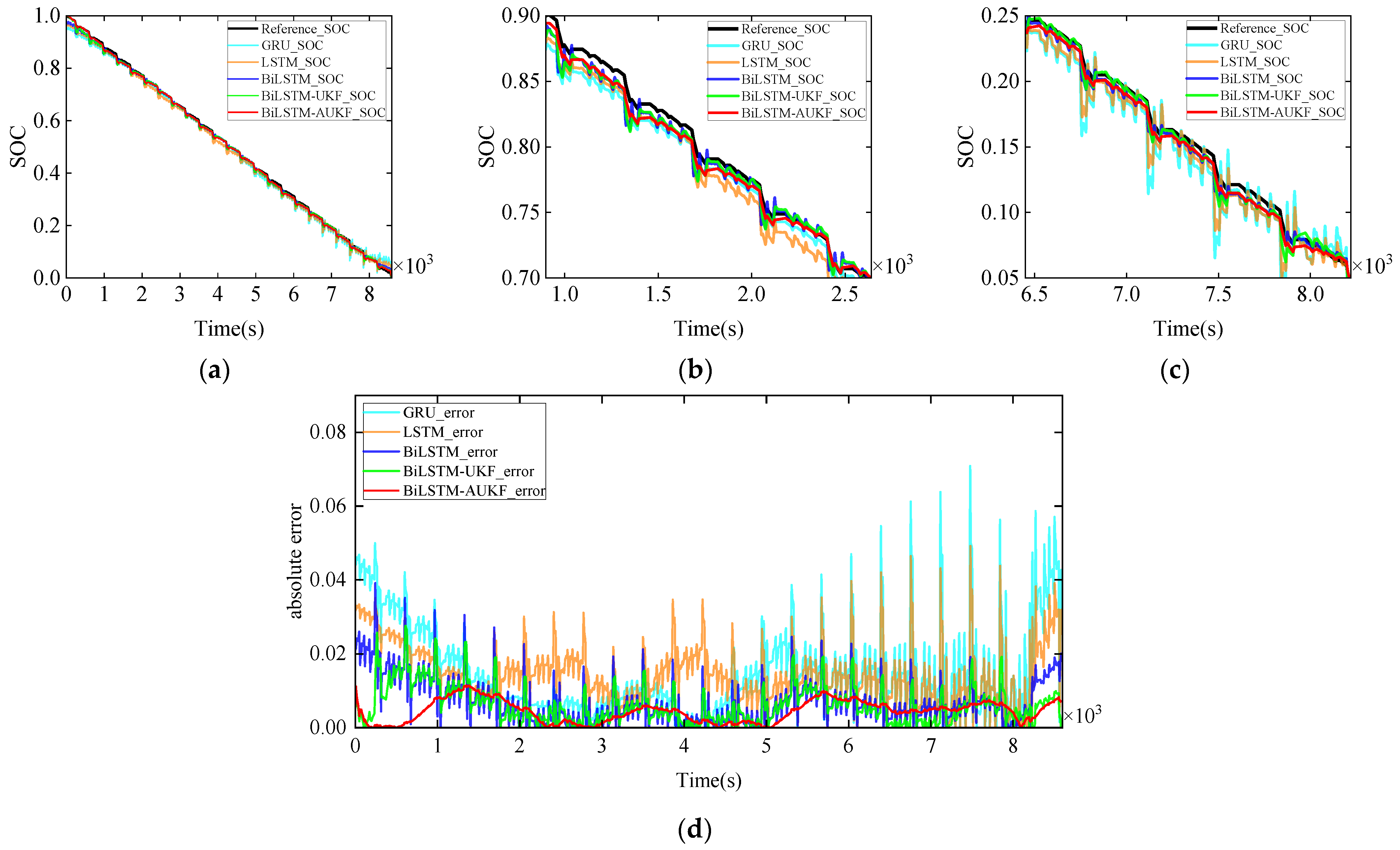
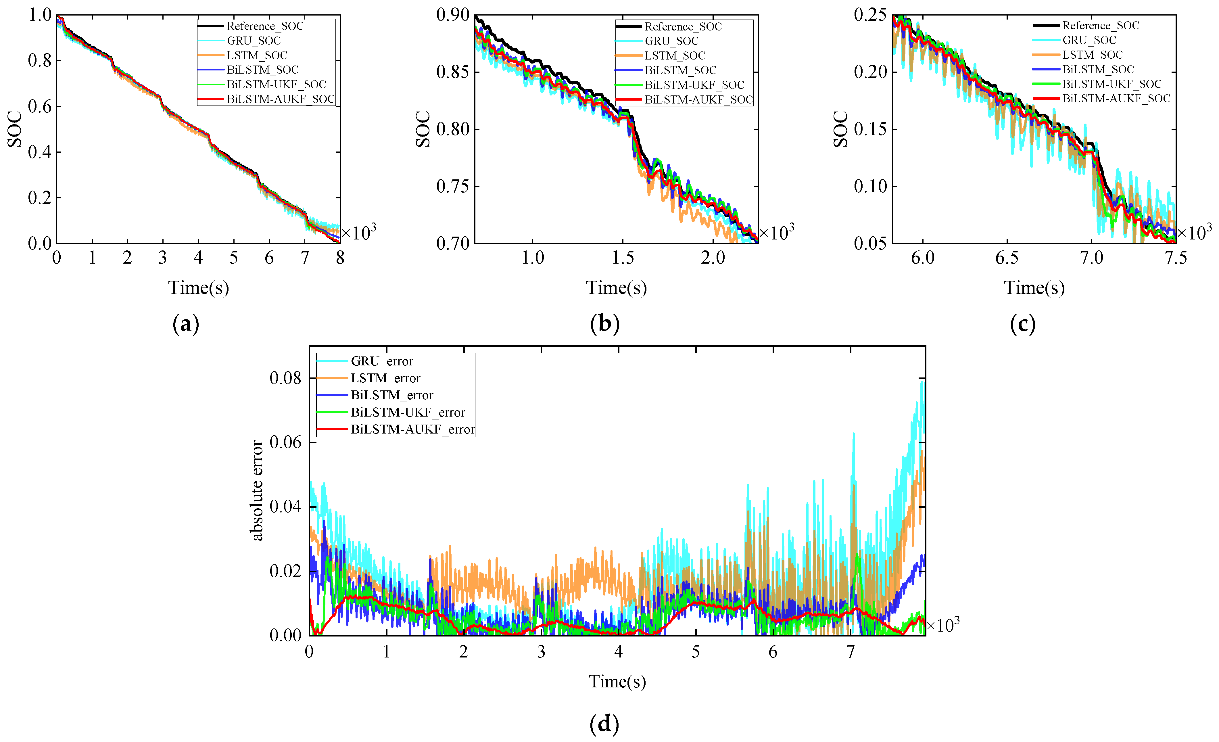
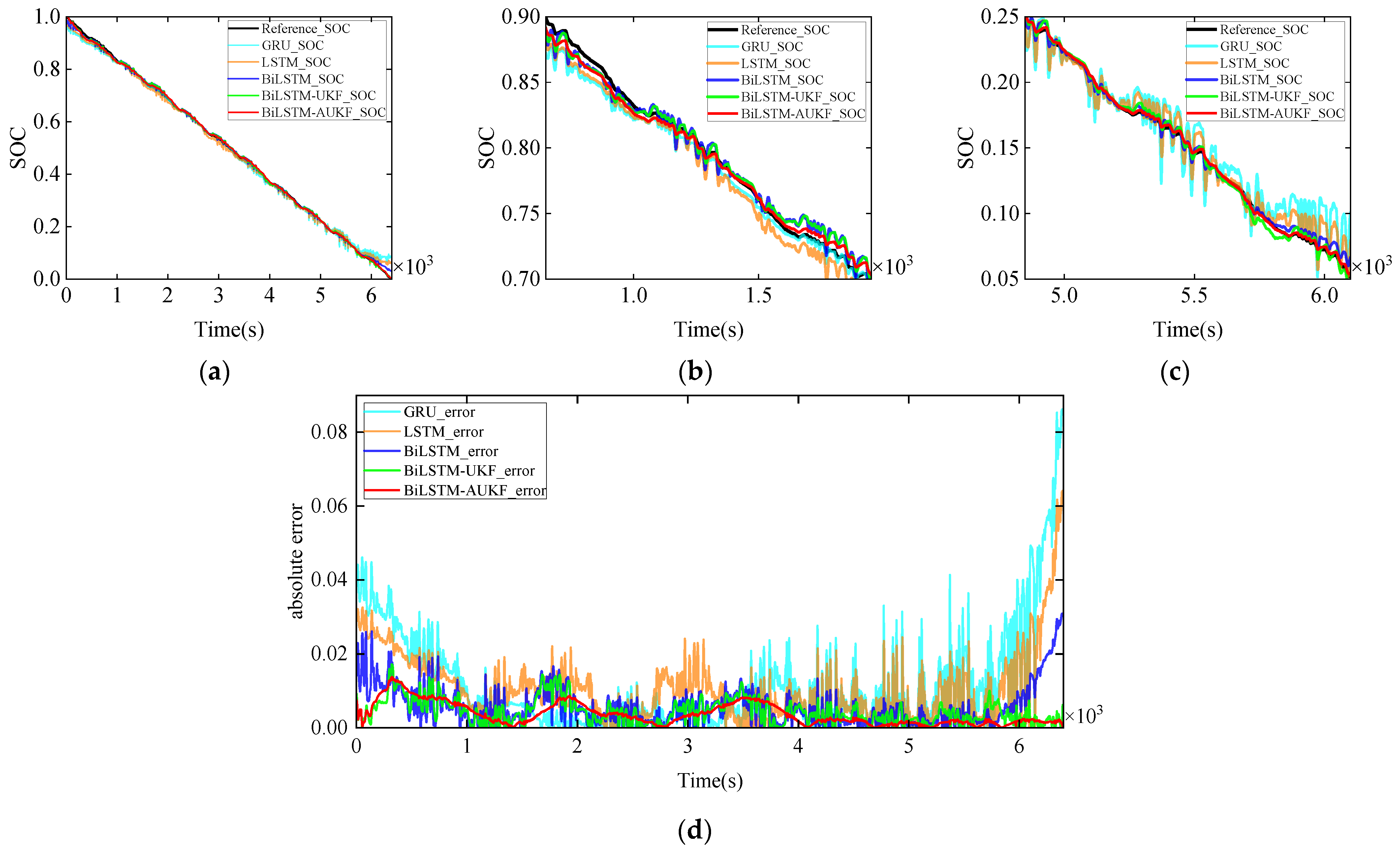
To verify the estimation accuracy of BiLSTM and the performance improvement effect of the Sage–Husa adaptive strategy on UKF, this study designed five comparative experiments: under a constant temperature of 20 °C, using the same DST, FUDS, and US06 driving cycle data, the GRU, LSTM, BiLSTM, BiLSTM-UKF, and BiLSTM-AUKF algorithms were, respectively, employed for SOC estimation. Notably, to ensure a rigorous evaluation of generalization performance under the cross-profile validation framework, each model was trained on a combination of the other two driving profiles, distinct from the testing profile. Specifically, models tested on DST (Figure 11 and Table 2) were trained on US06 and FUDS data; models tested on FUDS (Figure 12 and Table 3) were trained on DST and US06 data; and models tested on US06 (Figure 13 and Table 4) were trained on DST and FUDS data. In addition, all models were trained using multi-temperature operating condition data ranging from −10 °C to 50 °C. A 30-timestep sliding window and min-max normalization were applied for time-series reconstruction and preprocessing to enhance the models’ environmental adaptability and training efficiency. Figure 11, Figure 12 and Figure 13 present the estimation curves and error distributions of the five algorithms under the three driving cycles, while Table 2, Table 3 and Table 4 provide a quantitative comparison using three key metrics (MaxError, MAE, and RMSE), clearly quantifying the synergistic gains from bidirectional structure optimization and adaptive noise correction.
Comprehensive experimental evaluations confirm the superior estimation accuracy of the proposed BiLSTM-AUKF algorithm across diverse operating conditions compared to conventional methods such as GRU and LSTM. Under the dynamic stress test (DST) profile, for instance, the baseline GRU architecture yields an RMSE of 1.9514%, whereas the LSTM reduces this value to 1.6779%. The bidirectional LSTM structure demonstrates further improvement, achieving RMSE and MAE values of 0.94334% and 0.73297%, respectively, underscoring its enhanced capability in capturing temporal dependencies compared to unidirectional counterparts. Further refinement through the adaptive unscented Kalman filter culminates in the BiLSTM-AUKF hybrid model attaining RMSE and MAE values of 0.53123% and 0.44287%, corresponding to accuracy improvements of approximately 32.16% and 27.29% relative to the BiLSTM-UKF framework. These results substantiate that the synergistic integration of BiLSTM’s sophisticated feature extraction with AUKF’s robust filtering capacity produces a substantial enhancement in SOC estimation precision.
While estimation accuracy serves as the primary optimization objective, computational efficiency remains a crucial practical concern. As summarized in Table 5, a systematic evaluation was performed to assess the training and inference costs associated with different algorithmic architectures.
As shown in Table 5, a quantitative comparison of the computational efficiency of the algorithms was conducted under a strict cross-condition validation framework. Our analysis confirms that the superior estimation accuracy of the BiLSTM-AUKF model comes with a manageable increase in computational load. It is true that BiLSTM-based architectures demand more processing time than simpler GRU or LSTM networks. However, the critical refinement introduced by the AUKF contributes negligibly to the overall latency. This produces a highly favorable trade-off, as the algorithm achieves a decisive leap in estimation quality with significantly lower RMSE and MAE, at only a modest and manageable cost. In safety-critical BMS applications where precision is paramount, such an investment in computational resources is unequivocally justified.

7.4. Generalization Capability Validation for BiLSTM-AUKF-Based SOC Estimation

To further validate the robustness of the proposed BiLSTM-AUKF algorithm under inaccurate initial SOC conditions, experiments were conducted at 20 °C using the DST, FUDS, and US06 driving cycles with varied initial SOC settings. Notably, the experimental conditions remained consistent with those described in Section 7.3, with the only modification being the variation in initial SOC values. The true initial SOC was 100%, while the algorithm was initialized at 90%, 80%, and 70%, respectively. As shown in Figure 14, the BiLSTM-AUKF algorithm rapidly converges to the true SOC value despite initial inaccuracies, demonstrating exceptional robustness.
To systematically validate the temperature adaptability of the BiLSTM-AUKF algorithm across a wide thermal range, this study selected three characteristic temperature points: 0 °C, 10 °C, and 40 °C. Using full drive-cycle data (DST, FUDS, and US06) from the CALCE dataset, temperature robustness tests were conducted. It should be noted that the model training protocols remained identical to those described in Section 7.3, with the only extension being the incorporation of additional temperature test points. As detailed in Table 6, Table 7 and Table 8, three core metrics—MaxError, MAE, and RMSE—were statistically analyzed to quantify the algorithm’s precision degradation characteristics and stability boundaries under thermal stress, conclusively demonstrating its wide-temperature adaptation mechanism. Validation confirms that the proposed integrated algorithm achieves high-precision SOC estimation while maintaining robust performance across diverse environmental temperatures and operational conditions.

8. Conclusions

This paper proposes a high-precision SOC estimation method for lithium-ion batteries based on a BiLSTM-AUKF synergistic architecture. Experimental validation demonstrates that under diverse temperature environments and complex operating conditions, the BiLSTM-AUKF algorithm notably outperforms traditional Kalman filtering and neural network approaches in SOC estimation accuracy. Particularly under significant initial SOC errors, the algorithm exhibits exceptional convergence speed and robustness, rapidly approaching the true values. The BiLSTM’s powerful time-series feature extraction capability effectively compensates for model mismatch, while the Sage–Husa adaptive strategy dynamically adjusts the AUKF’s noise statistics, substantially reducing dependency on model and observation noise sensitivity. Consequently, this approach overcomes the limitations of conventional methods—parameter mismatch, error accumulation, and noise-induced accuracy degradation. The proposed method provides a novel framework for high-precision BMS, with its enhanced SOC estimation accuracy offering significant engineering value in optimizing energy management strategies and extending battery cycle life.
However, practical implementation in BMS faces challenges including high computational demands, generalization across diverse battery chemistries and aging states, and dynamic noise management. Future research should focus on developing lightweight algorithm versions, incorporating transfer learning for better adaptability, and enabling joint SOC-SOH estimation. Further validation under real electric vehicle operating conditions is equally essential for practical deployment.

Author Contributions

Conceptualization, R.W. and L.L.; methodology, R.W.; software, R.W.; validation, L.L., R.W., and F.Y.; formal analysis, H.Z., Q.Q. (Qifeng Qian), Q.Q. (Qiansheng Qiu) and L.X.; investigation, R.W., L.L., and C.T.; resources, R.W.; data curation, L.L. and R.W.; writing—original draft preparation, R.W. and L.L.; writing—review and editing, R.W. and F.Y.; visualization, L.L.; supervision, R.W. and C.T.; project administration, R.W.; funding acquisition, R.W. All authors have read and agreed to the published version of the manuscript.

Funding

This work was supported by the National Natural Science Foundation of China (grant number 62301086), the Natural Science Foundation of Jiangsu Province (grant number BK20230627), and the High-Level Talent Introduction Project of Changzhou University, China (grant number ZMF22020078).

Data Availability Statement

The original contributions presented in this study are included in the article. Further inquiries can be directed to the corresponding author.

Conflicts of Interest

Authors Rui Wang, Honghou Zhang, Qifeng Qian, Lingchao Xiao, Qiansheng Qiu were employed by the company Zhejiang Sunoren Solar Technology Co., Ltd. The remaining authors declare that the research was conducted in the absence of any commercial or financial relationships that could be construed as a potential conflict of interest.

References

  1. Hannan, M.A.; Lipu, M.S.H.; Hussain, A.; Mohamed, A. A review of lithium-ion battery state of charge estimation and management system in electric vehicle applications: Challenges and recommendations. Renew. Sustain. Energy Rev. 2017, 78, 834–854. [Google Scholar] [CrossRef]
  2. Wang, Y.; Zhang, X.; Li, K.; Zhao, G.; Chen, Z. Perspectives and challenges for future lithium-ion battery control and management. eTransportation 2023, 18, 100260. [Google Scholar] [CrossRef]
  3. Zhao, X.; Qian, X.; Xuan, D.; Jung, S. State of charge estimation of lithium-ion battery based on multi-input extreme learning machine using online model parameter identification. J. Energy Storage 2022, 56, 105796. [Google Scholar] [CrossRef]
  4. He, H.; Zhang, X.; Xiong, R.; Xu, Y.; Guo, H. Online model-based estimation of state-of-charge and open-circuit voltage of lithium-ion batteries in electric vehicles. Energy 2012, 39, 310–318. [Google Scholar] [CrossRef]
  5. Pillai, P.; Sundaresan, S.; Kumar, P.; Pattipati, K.R.; Balasingam, B. Open-Circuit Voltage Models for Battery Management Systems: A Review. Energies 2022, 15, 6803. [Google Scholar] [CrossRef]
  6. Zhang, X.; Duan, L.; Gong, Q.; Wang, Y.; Song, H. State of charge estimation for lithium-ion battery based on adaptive extended Kalman filter with improved residual covariance matrix estimator. J. Power Sources 2024, 589, 233758. [Google Scholar] [CrossRef]
  7. Shrivastava, P.; Soon, T.K.; Bin Idris, M.Y.I.; Mekhilef, S.; Adnan, S.B.R.S. Comprehensive co-estimation of lithium-ion battery state of charge, state of energy, state of power, maximum available capacity, and maximum available energy. J. Energy Storage 2022, 56, 106049. [Google Scholar] [CrossRef]
  8. Luan, Z.; Qin, Y.; Hu, B.; Zhao, W.; Wang, C. Estimation of state of charge for hybrid unmanned aerial vehicle Li-ion power battery for considering rapid temperature change. J. Energy Storage 2023, 59, 106479. [Google Scholar] [CrossRef]
  9. Wang, L.; Han, J.; Liu, C.; Li, G. State of charge estimation of lithium-ion based on VFFRLS-noise adaptive CKF algorithm. Ind. Eng. Chem. Res. 2022, 61, 22. [Google Scholar] [CrossRef]
  10. Li, S.; Li, Y.; Zhao, D.; Zhang, C. Adaptive state of charge estimation for lithium-ion batteries based on implementable fractional-order technology. J. Energy Storage 2020, 32, 101838. [Google Scholar] [CrossRef]
  11. Wu, C.; Hu, W.; Meng, J.; Xu, X.; Huang, X.; Cai, L. State-of-charge estimation of lithium-ion batteries based on MCC-AEKF in non-Gaussian noise environment. Energy 2023, 274, 127316. [Google Scholar] [CrossRef]
  12. Zhao, H.; Liao, C.; Zhang, C.; Wang, L.; Wang, L. State-of-charge estimation of lithium-ion battery: Joint long short-term memory network and adaptive extended Kalman filter online estimation algorithm. J. Power Sources 2024, 604, 234451. [Google Scholar] [CrossRef]
  13. Wu, S.; Pan, W.; Zhu, M. A collaborative estimation scheme for lithium-ion battery state of charge and state of health based on electrochemical model. J. Electrochem. Soc. 2022, 169, 090516. [Google Scholar] [CrossRef]
  14. Shen, D.; Ding, J.; Hao, T. Elman neural network and thevenin equivalent circuit model based multi-measurement Kalman filter for SOC estimation. Ionics 2024, 30, 833–845. [Google Scholar] [CrossRef]
  15. Dar, T.H.; Singh, S. Advanced integration of bidirectional long short-term memory neural networks and innovative extended Kalman filter for state of charge estimation of lithium-ion battery. J. Power Sources 2025, 628, 235893. [Google Scholar] [CrossRef]
  16. Monirul, I.M.; Qiu, L.; Ruby, R. Accurate SOC estimation of ternary lithium-ion batteries by HPPC test-based extended Kalman filter. J. Energy Storage 2024, 92, 112304. [Google Scholar] [CrossRef]
  17. Wang, M.; Wang, G.; Xiao, Z.; Sun, Y.; Zheng, Y. State of charge estimation of LiFePO4 in various temperature scenarios. Batteries 2023, 9, 43. [Google Scholar] [CrossRef]
  18. Li, H.; Fu, L.; Long, X.; Liu, L.; Zeng, Z. A hybrid deep learning model for lithium-ion batteries state of charge estimation based on quantile regression and attention. Energy 2024, 294, 130834. [Google Scholar] [CrossRef]
  19. Zhang, C.; Wang, S.; Yu, C.; Xie, Y.; Fernandez, C. Novel improved particle swarm optimization- extreme learning machine algorithm for state of charge estimation of lithium-ion batteries. Ind. Eng. Chem. Res. 2022, 6, 46. [Google Scholar] [CrossRef]
  20. Ma, L.; Zhang, T. Deep learning-based battery state of charge estimation: Enhancing estimation performance with unlabelled training samples. J. Energy Chem. 2023, 80, 48–57. [Google Scholar] [CrossRef]
  21. Che, Y.; Xu, L.; Teodorescu, R.; Hu, X.; Onori, S. Enhanced SOC estimation for LFP batteries: A synergistic approach using coulomb counting reset, machine learning, and relaxation. ACS Energy Lett. 2025, 63, 2. [Google Scholar] [CrossRef]
  22. Hao, X.; Wang, S.; Fan, Y.; Xie, Y.; Fernandez, C. An improved forgetting factor recursive least square and unscented particle filtering algorithm for accurate lithium-ion battery state of charge estimation. J. Energy Storage 2023, 59, 106478. [Google Scholar] [CrossRef]
  23. Wang, C.; Li, Q.; Tang, A.; Zhang, Z. A comparative study of state of charge estimation methods of ultracapacitors for electric vehicles considering temperature characteristics. J. Energy Storage 2023, 63, 106908. [Google Scholar] [CrossRef]
  24. El Fallah, S.; Kharbach, J.; Hammouch, Z.; Rezzouk, A.; Jamil, M.O. State of charge estimation of an electric vehicle’s battery using deep neural Networks: Simulation and experimental results. J. Energy Storage 2023, 62, 106904. [Google Scholar] [CrossRef]
  25. Liu, X.; Li, Q.; Wang, L.; Lin, M.; Wu, J. Data-driven state of charge estimation for power battery with improved extended Kalman filter. IEEE Trans. Instrum. Meas. 2023, 72, 1500910. [Google Scholar] [CrossRef]
  26. Wadi, A.; Abdel-Hafez, M.F.; Hussein, A.; Alkhawaja, F. Alleviating dynamic model uncertainty effects for improved battery SOC estimation of EVs in highly dynamic environments. IEEE Trans. Veh. Technol. 2021, 70, 6554–6566. [Google Scholar] [CrossRef]
  27. Zhang, X.; Hou, J.; Wang, Z.; Jiang, Y. Study of SOC estimation by the ampere-hour integral method with capacity correction based on LSTM. Batteries 2022, 8, 170. [Google Scholar] [CrossRef]
  28. Yang, F.; Zhang, S.; Li, W.; Miao, Q. State-of-charge estimation of lithium-ion batteries using LSTM and UKF. Energy 2020, 201, 117664. [Google Scholar] [CrossRef]
  29. Xu, K.; He, T.; Yang, P.; Meng, X.; Zhu, C.; Jin, X. A new online SOC estimation method using broad learning system and adaptive unscented Kalman filter algorithm. Energy 2024, 309, 132920. [Google Scholar] [CrossRef]
  30. Tian, J.; Xiong, R.; Lu, J.; Chen, C.; Shen, W. Battery state-of-charge estimation amid dynamic usage with physics-informed deep learning. Energy Storage Mater. 2022, 50, 718–729. [Google Scholar] [CrossRef]
  31. Takyi-Aninakwa, P.; Wang, S.; Liu, G.; Bage, A.N.; Masahudu, F.; Guerrero, J.M. An enhanced lithium-ion battery state-of-charge estimation method using long short-term memory with an adaptive state update filter incorporating battery parameters. Eng. Appl. Artif. Intell. 2024, 132, 107946. [Google Scholar] [CrossRef]
  32. Chen, Z.; Zhao, H.; Shu, X.; Zhang, Y.; Shen, J.; Liu, Y. Synthetic state of charge estimation for lithium-ion batteries based on long short-term memory network modeling and adaptive H-Infinity filter. Energy 2021, 228, 120630. [Google Scholar] [CrossRef]
  33. Wang, Q.; Ye, M.; Wei, M.; Lian, G.; Li, Y. Deep convolutional neural network based closed-loop SOC estimation for lithium-ion batteries in hierarchical scenarios. Energy 2023, 263, 125718. [Google Scholar] [CrossRef]
  34. Chen, J.; Zhang, Y.; Li, W.; Cheng, W.; Zhu, Q. State of charge estimation for lithium-ion batteries using gated recurrent unit recurrent neural net-work and adaptive Kalman filter. J. Energy Storage 2022, 55, 105396. [Google Scholar] [CrossRef]
  35. Wei, M.; Ye, M.; Zhang, C.; Lian, G.; Xia, B.; Wang, Q. Robust state of charge estimation of LiFePO4 batteries based on Sage-Husa adaptive Kalman filter and dynamic neural network. Electrochim. Acta 2024, 477, 143778. [Google Scholar] [CrossRef]
  36. Yang, Y.; Xu, Y.; Nie, Y.; Li, J.; Liu, S.; Zhao, L.; Yu, Q.; Zhang, C. Deep transfer learning enables battery state of charge and state of health estimation. Energy 2024, 294, 130779. [Google Scholar] [CrossRef]
  37. Tian, Y.; Lai, R.; Li, X.; Xiang, L.; Tian, J. A combined method for state-of-charge estimation for lithium-ion batteries using a long short-term memory network and an adaptive cubature Kalman filter. Appl. Energy 2020, 265, 114789. [Google Scholar] [CrossRef]
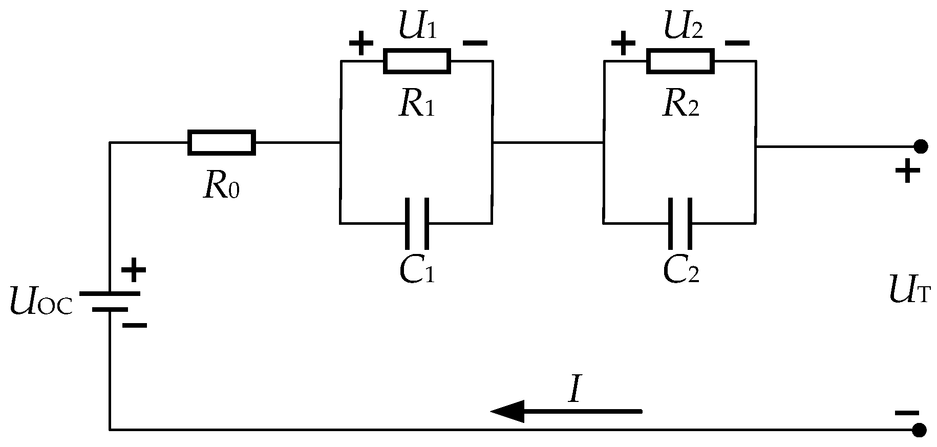
Figure 1. Second-Order RC equivalent circuit model.
Energies 18 05624 g001
Figure 2. Flowchart of battery SOC estimation using BiLSTM-AUKF fusion model.
Energies 18 05624 g002
Figure 3. Flowchart of PSO-based parameter identification for battery ECM.
Energies 18 05624 g003
Figure 4. Schematic diagram of BiLSTM information propagation.
Energies 18 05624 g004
Figure 5. Architecture of dual-input BiLSTM network.
Energies 18 05624 g005
Figure 6. BO workflow for the BiLSTM model.
Energies 18 05624 g006
Figure 7. AUKF iterative update flowchart.
Energies 18 05624 g007
Figure 8. OCV-SOC fitting curve comparison chart.
Energies 18 05624 g008
Figure 9. OCV-SOC fitting curve error analysis chart.
Energies 18 05624 g009
Figure 10. Comparative analysis of terminal voltage under FUDS driving.
Energies 18 05624 g010
Figure 11. SOC estimation results and errors with models trained on the combined US06 and FUDS datasets and tested on the DST profile: (a) SOC estimation for the entire DST working condition process; (b) partial enlarged view of the front section of (a); (c) partial enlarged view of the rear section of (a); (d) absolute error comparison across algorithms.
Energies 18 05624 g011
Figure 12. SOC estimation results and errors with models trained on the combined US06 and DST datasets and tested on the FUDS profile: (a) SOC estimation for the entire FUDS working condition process; (b) partial enlarged view of the front section of (a); (c) partial enlarged view of the rear section of (a); (d) absolute error comparison across algorithms.
Energies 18 05624 g012
Figure 13. SOC estimation results and errors with models trained on the combined DST and FUDS datasets and tested on the US06 profile: (a) SOC estimation for the entire US06 working condition process; (b) partial enlarged view of the front section of (a); (c) partial enlarged view of the rear section of (a); (d) absolute error comparison across algorithms.
Energies 18 05624 g013
Figure 14. SOC estimation with varying Initial values under driving cycles of (a) DST, (b) FUDS, and (c) US06.
Energies 18 05624 g014
Table 1. Model parameter identification results.
TemperatureR0 (Ω)R1 (Ω)C1 (F)R2 (Ω)C2 (F)
20 °C0.172060.014629651.42730.00126679683.0963
Table 2. SOC estimation error statistics under the DST test profile for models trained on the combined US06 and FUDS driving cycles.
Working ConditionsEstimation MethodMaxError/% MAE/% RMSE/%
DSTGRU7.08951.54941.9514
LSTM4.91881.49841.6779
BiLSTM3.91360.732970.94334
BiLSTM-UKF2.75220.609150.78313
BiLSTM-AUKF1.14460.442870.53123
Table 3. SOC estimation error statistics under the FUDS test profile for models trained on the combined US06 and DST driving cycles.
Working ConditionsEstimation MethodMaxError/% MAE/% RMSE/%
FUDSGRU7.88981.6012.1161
LSTM5.73381.54311.7605
BiLSTM3.5570.740940.93266
BiLSTM-UKF2.5320.588930.75801
BiLSTM-AUKF1.2650.526620.62845
Table 4. SOC estimation error statistics under the US06 test profile for models trained on the combined DST and FUDS driving cycles.
Working ConditionsEstimation MethodMaxError/% MAE/% RMSE/%
US06GRU8.62521.21651.8535
LSTM6.41481.07231.4226
BiLSTM3.08880.580340.78363
BiLSTM-UKF1.71880.438670.54656
BiLSTM-AUKF1.37680.370330.47677
Table 5. Efficiency comparison table.
AlgorithmTraining SetEpoch Time (s)Testing SetInference Time per Time Step (s)
GRUDST + FUDS67.33US060.0087387
DST + US0670.10FUDS0.008614
US06 + FUDS68.67DST0.0085396
LSTMDST + FUDS71.35US060.0090138
DST + US0673.40FUDS0.0089999
US06 + FUDS73.02DST0.008971
BiLSTMDST + FUDS74.45US060.013268
DST + US0676.67FUDS0.013047
US06 + FUDS76.49DST0.013134
BiLSTM-UKFDST + FUDS74.45US060.013296473
DST + US0676.67FUDS0.013074086
US06 + FUDS76.49DST0.013159713
BiLSTM-AUKFDST + FUDS74.45US060.013297232
DST + US0676.67FUDS0.013075712
US06 + FUDS76.49DST0.013164777
Table 6. SOC estimation errors for different driving cycles at 0 °C.
Working ConditionEstimation MethodMaxError/% MAE/% RMSE/%
DSTLSTM4.60871.4671.6347
BiLSTM3.31730.717320.89197
BiLSTM-UKF2.63820.702040.86481
BiLSTM-AUKF1.60010.516540.61679
FUDSLSTM6.22051.40441.6845
BiLSTM3.3150.644640.85691
LSTM-UKF2.90590.615860.80715
BiLSTM-AUKF2.16480.42340.54408
US06LSTM4.89381.00871.3199
BiLSTM2.38270.524170.69309
LSTM-UKF2.63920.487360.6562
BiLSTM-AUKF1.69450.311240.39664
Table 7. SOC estimation errors for different driving cycles at 10 °C.
Working ConditionEstimation MethodMaxError/% MAE/% RMSE/%
DSTLSTM4.95951.63231.8089
BiLSTM3.40980.794090.97419
BiLSTM-UKF2.69180.777230.94338
BiLSTM-AUKF1.93290.605880.72084
FUDSLSTM4.46451.49651.6572
BiLSTM3.42870.707290.88551
LSTM-UKF2.77740.690090.8514
BiLSTM-AUKF1.46380.577140.68095
US06LSTM6.19011.16091.5187
BiLSTM2.91150.557830.76841
LSTM-UKF1.7680.419380.52105
BiLSTM-AUKF1.33770.334960.43993
Table 8. SOC estimation errors for different driving cycles at 40 °C.
Working ConditionEstimation MethodMaxError/% MAE/% RMSE/%
DSTLSTM5.79291.49621.7191
BiLSTM3.55190.714530.92059
BiLSTM-UKF2.43960.547140.7102
BiLSTM-AUKF0.944160.407770.47844
FUDSLSTM6.09391.52511.7302
BiLSTM3.53850.714470.91028
LSTM-UKF2.50370.575980.71939
BiLSTM-AUKF1.17280.478130.56799
US06LSTM6.00551.19431.5234
BiLSTM2.72870.570780.76258
LSTM-UKF1.63060.469820.56751
BiLSTM-AUKF1.10430.357830.45392
Disclaimer/Publisher’s Note: The statements, opinions and data contained in all publications are solely those of the individual author(s) and contributor(s) and not of MDPI and/or the editor(s). MDPI and/or the editor(s) disclaim responsibility for any injury to people or property resulting from any ideas, methods, instructions or products referred to in the content.