Self-Supervised Representation Learning for UK Power Grid Frequency Disturbance Detection Using TC-TSS

Abstract

This study presents a self-supervised learning framework for detecting frequency disturbances in power systems using high-resolution time series data. Employing data from the UK National Grid, we apply the Temporal Contrastive Self-Supervised Learning (TC-TSS) approach to learn task-agnostic embeddings from unlabelled 60-s rolling window segments of frequency measurements. The learned representations are then used to train four traditional classifiers, Logistic Regression (LR), Support Vector Machine (SVM), Multi-Layer Perceptron (MLP), and Random Forest (RF), for binary classification of frequency stability events. The proposed method is evaluated using over 15 million data points spanning six months of system operation data. Results show that classifiers trained on TC-TSS embeddings performed better than those using raw input features, particularly in detecting rare disturbance events. ROC-AUC scores for MLP and SVM models reach as high as 0.98, indicating excellent separability in the latent space. Visualisations using UMAP and t-SNE further demonstrate the clustering quality of TC-TSS features. This study highlights the effectiveness of contrastive representation learning in the energy domain, particularly under conditions of limited labelled data, and proves its suitability for integration into real-time smart grid applications.

1. Introduction

The National Energy System Operator (NESO) is responsible for the long-term planning and real-time operation of the electricity and gas networks in Great Britain [1,2]. NESO ensures secure and reliable energy supply, promotes efficient system operation, and plays a key role in supporting the UK’s transition to net-zero emissions [3]. One of its critical responsibilities is maintaining frequency stability, which underpins the operational resilience of modern power systems [4]. This challenge is particularly pronounced in low-inertia grids like the UK’s, where the increasing penetration of renewable energy sources makes the grid more sensitive to disturbances [5,6]. Frequency deviations caused by load-generation imbalances, sudden generation loss, or equipment faults can trigger cascading failures if not detected and mitigated promptly [7].

Traditional frequency monitoring approaches heavily rely on rule-based thresholds and handcrafted statistical features [8]. While effective in identifying large-scale events, these methods often struggle to detect subtle or emerging disturbances in real time, especially under evolving grid conditions. To address these limitations, machine learning (ML) and deep learning (DL) methods have recently been introduced for power system event detection. For example, convolutional and recurrent neural networks have been employed to classify transient disturbances and predict stability margins [9], and transformer-based architectures have shown promise in capturing long-range temporal dependencies in system dynamics [10]. Despite their success, most of these supervised methods depend on large, labelled datasets that are often unavailable in real-world grid operations, where disturbance events are relatively rare compared to normal operating conditions.

2. Literature Review

Supervised machine learning methods have shown promise in automating disturbance detection and classification tasks [11]. However, they typically rely on large volumes of labelled training data—a requirement rarely satisfied in real-world grid operations. Events such as islanding and under-frequency excursions are rare and underrepresented in most public datasets, making it difficult to train reliable models. Furthermore, the manual labelling of high-resolution time series data is time-consuming and not feasible for real-time deployment [12].

Deep learning models, including convolutional neural networks (CNNs) and recurrent architectures such as long short-term memory (LSTM) [13,14,15], have also been explored for grid frequency prediction and anomaly detection [16,17]. Nonetheless, these models are susceptible to prediction errors due to oversimplified assumptions that often ignore load dynamics and network topology [18].

To address the challenges of limited labelled data and the high cost of manual annotation, self-supervised representation learning (SSRL) has emerged as a powerful alternative. SSRL enables models to learn rich and generalisable feature representations directly from unlabelled data [19], making it particularly suitable for time series analysis in domains such as energy systems. These representations can be transferred to a variety of downstream tasks, including classification, forecasting, anomaly detection, and fault diagnosis [20,21].

In recent years, SSRL has proven especially effective for time series analysis where labelled events are scarce. Methods such as Contrastive Predictive Coding (CPC) [22], SimCLR [23], TS-TCC [24], TimeContrast [25], and masked autoencoders [26] have demonstrated the ability to learn robust and transferable representations without extensive labelled data. By using pretext tasks—such as temporal contrasting, augmentation-based invariance, and masked prediction—these frameworks capture both global and local dynamics in sequential signals and have achieved state-of-the-art performance across multiple domains. Contrastive learning, in particular, maximises agreement between augmented views of the same input while distinguishing them from others, thereby learning discriminative embeddings. In the power systems domain, such approaches reduce reliance on expert labelling while maintaining competitive accuracy in temporal signal interpretation [27,28]. A typical time–frequency contrastive learning pipeline follows a pre-training and downstream design, enabling models to extract multi-perspective features from unlabelled data and fine-tune them for specific tasks. This paradigm has been successfully applied in related areas such as few-shot bearing fault diagnosis [29] and Short-Time Fourier Neural Networks (STFNets), which operate directly in the frequency domain using self-supervised learning to analyse sensing signals [30]. Such methods eliminate the need for costly manual labelling while supporting the development of reusable encoders across downstream applications [31].

Inspired by these developments, this study explores the use of Temporal Contrastive Self-Supervised Learning (TC-TSS) [32] to analyse frequency dynamics in power systems, enabling robust classification of disturbances without reliance on labelled training data. While SSRL has gained traction in other time series domains, it remains largely unexplored for power system frequency data in the UK context [33]. Public datasets typically lack labelled examples of critical events such as islanding, generation loss, or system faults. Moreover, these events are inherently rare and underrepresented, making it difficult to train supervised models effectively.

However, a critical research gap persists in developing label-efficient and adaptive models that can generalise across evolving grid conditions. Existing supervised approaches depend heavily on extensive labelled datasets and handcrafted features, which limit their scalability and responsiveness to dynamic operational environments. Manual annotation of frequency disturbances in operational data is labour-intensive, time-consuming, and impractical for real-time deployment, especially in low-inertia grids like the UK’s, where rapid fluctuations are more frequent [34]. As a result, existing supervised pipelines fall short in addressing the practical needs of grid operators [35].

To address this gap, this research proposes and evaluates TC-TSS as a robust, label-efficient alternative for frequency disturbance detection in the smart grid. By leveraging contrastive self-supervision, TC-TSS learns invariant temporal representations directly from unlabelled frequency data, enabling the detection of both known and unseen disturbances without manual labelling or prior fault definitions.

Contribution

The main contributions of this work are as follows:

• We propose a Temporal Contrastive Self-Supervised Learning (TC-TSS) framework that learns discriminative and invariant temporal features directly from unlabelled frequency data, addressing the limitations of existing supervised methods that rely on large annotated datasets.
• We demonstrate that TC-TSS features outperform raw inputs, achieving higher classification accuracy and perfect ROC-AUC (1.00) with nonlinear models such as SVM and MLP.
• By applying temporal data augmentations (noise, scaling, shifting, and reordering), the framework learns robust invariances that support detection of both known and unseen disturbances.
• The approach is validated on real UK National Grid frequency data, using over 15 million measurements collected at a 1-s resolution across six months, ensuring practical relevance.

In summary, this work introduces a label-efficient TC-TSS framework that learns robust features from unlabelled frequency data, improves detection accuracy over existing methods, and provides a flexible encoder that can be reused for real-time smart grid applications.

3. Materials and Methods

A self-supervised learning pipeline was implemented using contrastive learning to extract meaningful latent representations from frequency time series data, followed by downstream classification using standard machine learning models.

3.1. Data Details

The dataset used in this study comprises high-resolution system frequency measurements obtained from the National Grid ESO’s publicly available system data portal. Frequency values were recorded at a 1-s sampling rate, yielding 86,400 data points per day. The dataset spans six months from January 2025 to June 2025, covering recent operational conditions.

In total, the dataset includes approximately 15.5 million timestamped frequency measurements (2,592,000 per month), providing comprehensive temporal coverage suitable for time series analysis and disturbance classification. This high temporal resolution enables fine-grained characterisation of frequency dynamics within the UK power grid.

Figure 1 shows a time series plot of UK grid frequency data for June 2025, sampled at a 1-s resolution. The frequency fluctuates around the nominal 50 Hz value, exhibiting short-term variability and occasional sharp deviations, including brief under-frequency events dropping below 49.8 Hz. The plot displays a total of 2,592,000 data points over the 30 days, capturing the continuous operational dynamics of the power system.

3.2. Data Labelling

Under normal operating conditions, power system frequency is maintained within a statutory range of ±0.5 Hz around the nominal 50 Hz, as deviations beyond this threshold can lead to system instability, including brownouts or blackouts. To capture and analyse such critical variations, it is essential to define a practical operational limit that reflects frequency stability boundaries.

For the purpose of this study, frequency values within the range of 49.8 Hz to 50.2 Hz are considered normal, representing stable grid operation. Data points falling outside this range are labelled as disturbance events, indicating potential anomalies or stress conditions within the grid. This binary labelling facilitates the development and evaluation of models for frequency stability analysis and disturbance detection.

3.3. Feature Generation

To extract temporal features that capture dynamic trends in the frequency signal, a rolling window approach was employed. Specifically, a 60-s sliding window was applied across the time series data, generating overlapping sequences of frequency values.

Each window contains 60 data points (1-s resolution), and features were computed across these windows to encapsulate short-term variations. The resulting feature matrix has a dimension of 260,640 × 62, where 260,640 corresponds to the total number of generated windows, and 62 represents the number of features, including the raw frequency values within each window and timestamp and data labelling.

The 60-s rolling window was selected based on operational characteristics of the UK power grid, where frequency control actions and primary response mechanisms typically occur within a 1-min timescale. This duration is long enough to capture complete transient and recovery behaviours following small disturbances yet short enough to preserve temporal locality for data-driven models. Preliminary trials with shorter windows (30 s) led to fragmented disturbance patterns, while longer windows (120 s) increased data redundancy without improving classification performance. Therefore, the 60-s window provides an effective balance between temporal resolution and contextual coverage for event representation.

3.4. Temporal Contrastive Self-Supervised Learning (TC-TSS)

To understand robust temporal representations from high-resolution frequency data, we employed the Temporal Contrastive Self-Supervised Learning (TC-TSS) framework. TC-TSS is specifically designed for time series by using contrastive objectives over temporally augmented signal pairs. The method enables representation learning from unlabelled sequences, making it highly suitable for system frequency data where disturbance events are rare and labels are expensive.

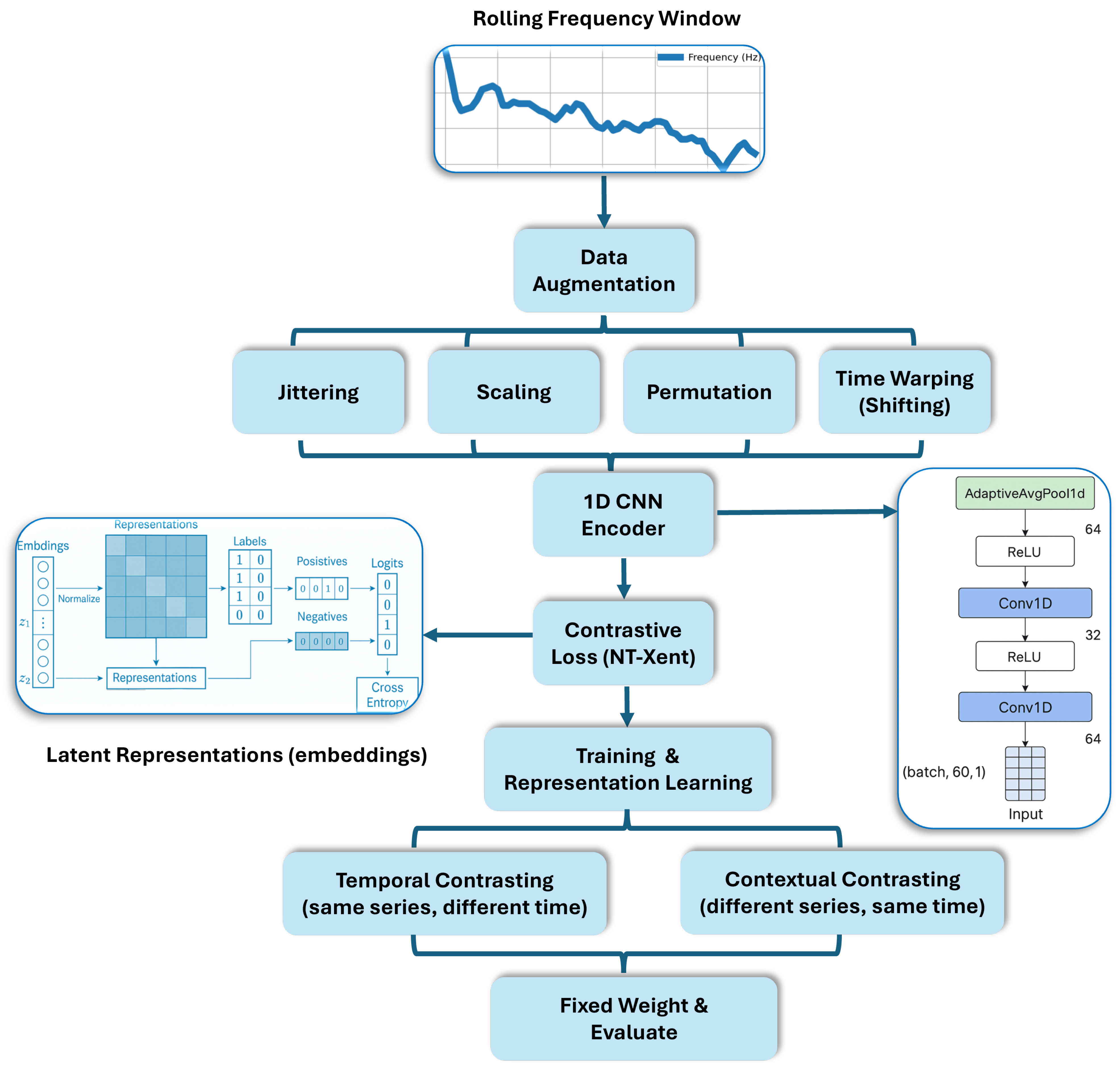
From a theoretical standpoint, power system frequency deviations reflect the system’s inertia and damping characteristics, which manifest as correlated temporal patterns. TC-TSS seeks to maximise mutual information between temporally adjacent views of the same signal window, thereby preserving dynamic invariants that correspond to underlying physical stability modes. This formulation can be interpreted as learning a mapping $f_{\theta }:{\mathbb{R}}^T\to {\mathbb{R}}^d$ that linearises nonlinear temporal dependencies through contrastive alignment of augmented trajectories. A concise design framework is shown in Figure 2.

TC-TSS consists of three major steps:

• Data augmentation ≈ simulate stochastic perturbations of frequency behaviour.
• Encoder (CNN Encoder) ≈ nonlinear function extractor approximating temporal convolution over frequency response.
• Contrastive loss (with NT-Xent) ≈ enforces invariance to augmentation and discrimination of dynamics.

Data Augmentation: To improve generalisation and robustness, a custom FrequencyDataset class was defined to include time series augmentations during contrastive training. These augmentations involved additive Gaussian noise, amplitude scaling, random permutation of signal segments, and temporal shifting to create augmented positive pairs.

Given an input frequency window $x\in {\mathbb{R}}^T$ of length $T=60$ s, two stochastic augmentations ${\mathcal{A}}_1$ and ${\mathcal{A}}_2$ are applied to generate two correlated views $({\tilde{x}}_1,{\tilde{x}}_2)$:

$${\tilde{x}}_1={\mathcal{A}}_1\left(x\right),{\tilde{x}}_2={\mathcal{A}}_2\left(x\right)$$

(1)

The pair $({\tilde{x}}_1,{\tilde{x}}_2)$ forms a positive pair, while other samples in the batch are treated as negative examples. These augmentations simulate natural stochastic perturbations—measurement noise, amplitude variation, or phase shifts—thus encouraging the encoder to focus on intrinsic temporal structure rather than superficial fluctuations.

The chosen temporal augmentations—additive Gaussian noise, amplitude scaling, segment permutation, and temporal shifting—were designed to emulate realistic perturbations observed in grid frequency measurements. Noise injection represents sensor or communication noise; amplitude scaling reflects variations in system inertia and damping; segment permutation encourages temporal invariance to minor reordering of oscillatory components; and temporal shifting models phase misalignment across measurement intervals. These augmentations were selected after preliminary tests showed that excluding any single transformation slightly reduced the contrastive loss convergence rate and final AUC (by up to 0.04), indicating their collective contribution to robust feature learning.

CNN Encoder Architecture: A lightweight 1D convolutional neural network (CNN) encoder was adopted to map each 60-point frequency window into a latent representation. The architecture included stacked 1D convolutional layers with ReLU activations followed by adaptive average pooling to produce fixed-length embeddings. This encoder structure is consistent with prior TC-TSS applications where local temporal patterns are essential for effective feature extraction. The architecture includes the following:

The CNN encoder maps a 1D input sequence $x\in {\mathbb{R}}^T$ to a latent representation $z\in {\mathbb{R}}^d$ through successive convolution and pooling operations:

$$z=\mathrm{AdaptiveAvgPool}1\mathrm{D}\left(\sigma \left({\mathrm{Conv}}_2\left(\sigma \left({\mathrm{Conv}}_1\left(x\right)\right)\right)\right)\right)$$

(2)

where ${\mathrm{Conv}}_1$ and ${\mathrm{Conv}}_2$ are 1D convolutional layers, $\sigma (·)$ denotes the ReLU activation, and AdaptiveAvgPool1D reduces the temporal dimension to 1. The resulting vector z is a compact embedding used in contrastive training. The encoder extracts localised temporal filters analogous to frequency response modes of the system. The resulting embedding therefore captures both short-term oscillatory behaviour and long-term stability signatures.

Contrastive Loss with NT-Xent: The encoder was trained using the NT-Xent loss (Normalised Temperature-scaled Cross-Entropy Loss), which encourages the embeddings of positive pairs to be similar while pushing apart representations of negative pairs. The contrastive objective encourages positive pairs to be similar and negative pairs to be dissimilar in the embedding space. The NT-Xent is used, defined for a batch of N-positive pairs (i.e., $2N$ total samples) as follows:

$${\mathcal{L}}_{i,j}=-log{\displaystyle \frac{exp(\mathrm{sim}({\widehat{z}}_i,{\widehat{z}}_j)/\tau )}{{\sum }_{k=1}^{2N}{⊮}_{[k\ne i]}exp(\mathrm{sim}({\widehat{z}}_i,{\widehat{z}}_k)/\tau )}}$$

(3)

where

• $\mathrm{sim}(u,v)=u^{\top }v$ is the cosine similarity;
• $\tau >0$ is a temperature hyperparameter;
• ${⊮}_{[k\ne i]}$ is an indicator function that excludes the anchor sample from the denominator.

The total contrastive loss across the batch is given by the following:

$$\mathcal{L}={\displaystyle \frac{1}{2N}}\sum _{i=1}^N\left({\mathcal{L}}_{2i-1,2i}+{\mathcal{L}}_{2i,2i-1}\right)$$

(4)

The NT-Xent objective approximates the maximisation of mutual information $I(Z_i,z_j)$ between positive temporal views. By constraining embeddings onto a unit hypersphere, the loss enforces angular separation between dissimilar trajectories and compactness among similar ones. Analytically, this produces a feature manifold where stable and disturbed frequency regimes occupy distinct subspaces—an outcome consistent with observed UMAP and t-SNE separability.

Encoder Training and Embedding Standardisation: The encoder was trained from scratch unless a pre-trained model was available. During training, the encoder parameters were updated using the Adam optimiser. At the end of training, the encoder weights were saved for reuse. The encoder was then used in evaluation mode to generate embeddings for both training and test datasets. The extracted embeddings were standardised to ensure zero mean and unit variance.

Once training is complete, the encoder $f_{\theta }$ can be used to generate fixed-length embeddings for any unseen input sequence. These embeddings are then used as input features for downstream classification tasks, enabling accurate and label-efficient detection of frequency disturbance events.

$$z=f_{\theta }\left(x\right)$$

(5)

The analytical perspective of the TC-TSS framework can be interpreted as an information–theoretic optimisation problem where the encoder $f_{\theta }$ learns to maximise mutual information between temporally consistent representations $z_i$ and $z_j$. By enforcing cosine similarity through the NT-Xent loss, the model constructs an embedding manifold in which similar temporal dynamics (e.g., stable frequency oscillations) are projected close together, whereas disturbance patterns are projected farther apart. This yields a feature space that preserves temporal continuity and enhances anomaly separability—a property directly aligned with the frequency stability characteristics of the grid.

3.5. Classification and Evaluation

The learned embeddings obtained from the TC-TSS encoder were used as input features for downstream supervised classification. Four widely used classifiers were selected for this task: Logistic Regression, Support Vector Machine (SVM), Multi-Layer Perceptron (MLP), and Random Forest. Given the inherent class imbalance in the dataset, where disturbance events are significantly less frequent than normal operation, a balanced classification setting was applied across models to mitigate bias toward the majority class.

Logistic Regression: Logistic Regression has been implemented using the “balanced” parameter, to adjust class weights inversely proportional to class frequencies in the input data, ensuring that disturbance samples are not underrepresented during model optimisation.

Support Vector Machine (SVM): An SVM with a radial basis function (RBF) kernel was also employed with a balance parameter to penalise the misclassification of minority-class samples and promote a more equitable decision boundary.

Multi-Layer Perceptron (MLP): A two-layer neural network with hidden layer sizes of (64, 32) was implemented. Although this model does not directly support class weight, its learning behaviour was evaluated under the same class imbalance conditions, and performance was compared with the balanced models.

Random Forest: A 100-tree ensemble Random Forest classifier was trained with the same balanced settings to correct for label distribution disparity. This forces the model to give higher importance to the disturbance class during tree construction.

Nonlinear classifiers such as SVM and MLP were selected because TC-TSS embeddings are distributed on curved manifolds; thus, nonlinear kernels or multilayer projections are theoretically capable of capturing margin boundaries that linear models cannot.

The performance of each model was assessed using standard metrics: accuracy, precision, recall, F1-score, and ROC-AUC. Additionally, we facilitated the granular analysis of true positives, false positives, and false negatives across both classes.

4. Results

4.1. Embedding Visualisation with UMAP and t-SNE

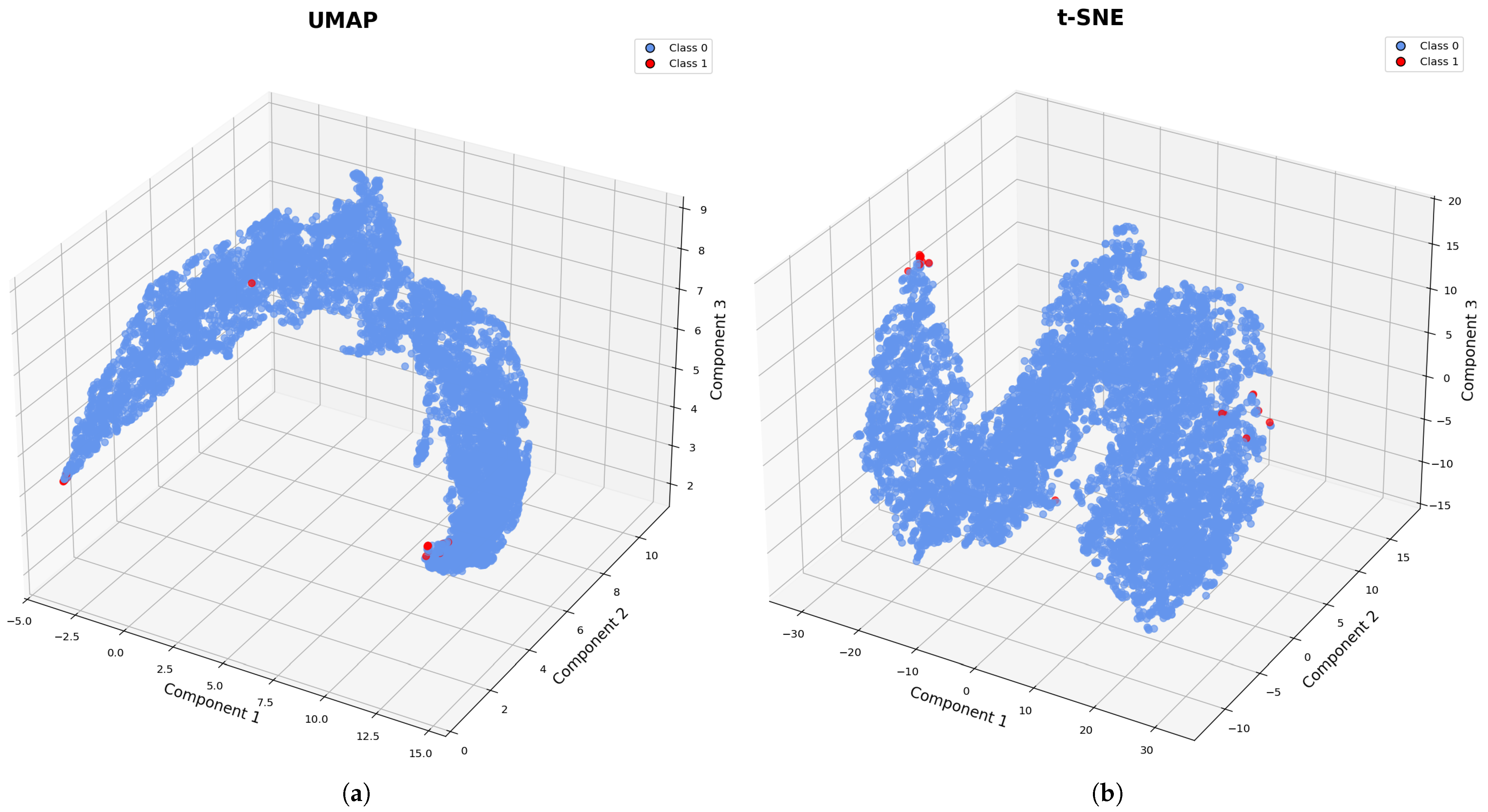
To gain qualitative insight into the structure of the learned feature representations, we employed two nonlinear dimensionality reduction techniques: Uniform Manifold Approximation and Projection (UMAP) and t-distributed Stochastic Neighbour Embedding (t-SNE). Both methods were applied to the 64-dimensional TC-TSS embeddings generated from the test set, projecting them into a 3D space for visualisation. In both cases, frequency windows labelled as normal (class 0) and disturbance (class 1) were coloured blue and red, respectively.

Figure 3a for UMAP shows a continuous and curved manifold where normal operating points cluster densely, and disturbance events appear as outliers at the boundaries or in sparsely populated regions. This indicates that the TC-TSS encoder effectively separates subtle anomalies in a mostly homogeneous space, whereas Figure 3b for t-SNE presents a more discrete, clustered embedding, where disturbance points are again well isolated from the majority of normal points. The preservation of local structure by t-SNE highlights the encoder’s ability to concentrate semantically similar representations in the latent space.

These visualisations provide further evidence that the TC-TSS model captures class-discriminative temporal features, even in the absence of supervision during training. The spatial separability of disturbance events supports the effectiveness of contrastive learning for anomaly detection in high-resolution frequency data.

From a grid dynamics perspective, the distinct clusters observed in the embedding space correspond to different operational regimes of the power system. The dense blue cluster represents stable operation, where system frequency remains tightly regulated around 50 Hz through governor and primary control actions. The red clusters at the boundaries correspond to transient or disturbed conditions, typically associated with rapid frequency deviations caused by sudden generation loss, load imbalance, or low-inertia responses. The gradual transitions between these regions indicate that the TC-TSS embeddings capture not only discrete event boundaries but also the intermediate recovery phases following disturbances. This physical interpretability confirms that the learned latent space encodes meaningful frequency behaviour consistent with real-world grid stability dynamics.

4.2. Experimental Configuration

The frequency time series was segmented into overlapping 60-s windows using a rolling window approach. Each window was labelled as either normal or disturbance based on whether its values remained within the statutory operational limits (49.8 Hz to 50.2 Hz). These segments were stored in a structured CSV file and reshaped to match the input format expected by the 1D CNN encoder.

The dataset was divided into training and testing subsets using an 80/20 split to preserve class distribution. To ensure robustness and evaluate generalisation, an additional 5-fold stratified cross-validation was conducted on the TC-TSS embeddings. The mean ROC-AUC across folds was 0.978 ± 0.018 for SVM and 0.973 ± 0.042 for MLP, confirming consistent performance across partitions and ruling out overfitting to a single train–test split, as shown below in

Table 1. Five-fold cross-validation results showing the mean and standard deviation of ROC-AUC for all evaluated classifiers.

Model	Mean AUC	Std AUC
Logistic Regression (balance)	0.5756	0.0457
SVM (RBF, balance)	0.9781	0.0180
MLP (balance)	0.9729	0.0422
Random Forest	0.9621	0.0409

.

The 1D CNN encoder comprised three convolutional blocks followed by an adaptive average-pooling layer and a fully connected projection head. Each block consisted of a 1D convolution, batch normalisation, ReLU activation, and max-pooling. Specifically, the convolutional layers used filter sizes of 5, 3, and 3 with 32, 64, and 128 filters, respectively. The projection head mapped the pooled feature vector to a 64-dimensional latent space. The total number of trainable parameters was approximately 0.42 million, ensuring a lightweight model suitable for large-scale time series data. Training was performed using the Adam optimiser (learning rate = 0.001, ${\beta }_1$ = 0.9, ${\beta }_2$ = 0.999) with a batch size of 128 and contrastive temperature parameter $\tau =0.5$. The encoder was trained for 10 epochs during self-supervised pre-training, with the NT-Xent loss consistently decreasing across epochs, indicating stable convergence.

Once training was complete, the encoder was used to extract fixed-length embeddings for all samples. These embeddings were standardised and then used as input features for downstream classification. For consistency and fairness, all traditional classifiers were trained and evaluated using the same data splits and preprocessing steps as the TC-TSS pipeline.

4.3. Model Comparison

To rigorously assess the discriminative capability of the learned representations, four machine learning classifiers—Logistic Regression, Support Vector Machine (RBF), Multi-Layer Perceptron (MLP), and Random Forest—were trained on two distinct feature sets: (1) the raw 60-s rolling window features and (2) embeddings extracted from the proposed TC-TSS framework. All models used identical configurations, including 5-fold stratified cross-validation, balanced class weights, and standardised inputs, ensuring a fair comparison of feature quality and model robustness.

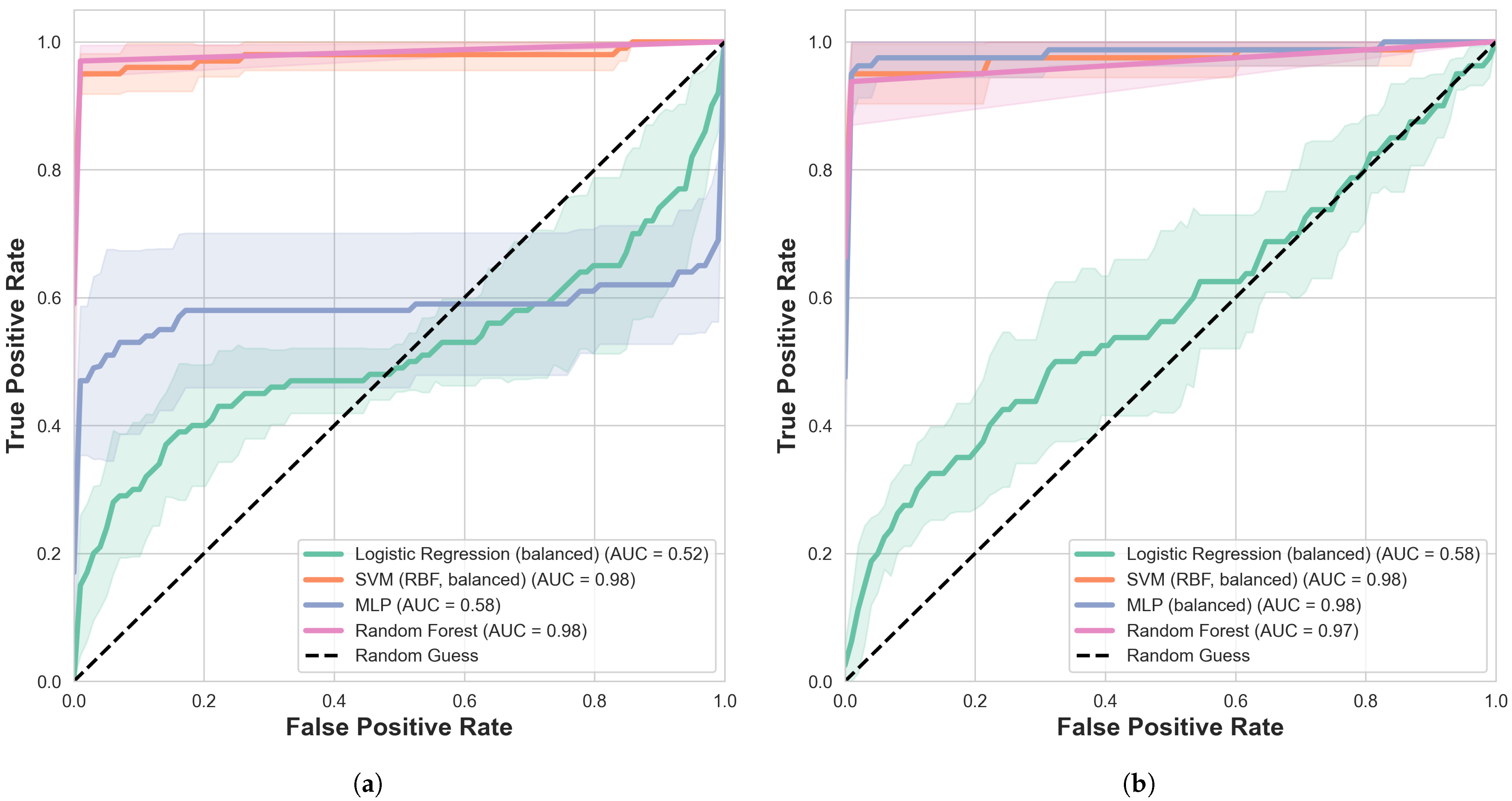
Figure 4a shows the ROC curves obtained from classifiers trained on raw input features, while Figure 4b presents the corresponding results using TC-TSS embeddings. The plots illustrate the mean ROC curves across 5-fold stratified cross-validation, with shaded regions indicating ±1 SD.

Across repeated runs and 5-fold cross-validation, the TC-TSS embeddings consistently enhanced classifier separability compared with models trained on raw input features. As shown in Figure 4b, both the SVM and MLP achieved near-optimal discrimination (AUC ≈ 0.98), while Random Forest also performed strongly (AUC ≈ 0.97). In contrast, Logistic Regression produced a substantially lower AUC (≈0.58), confirming that linear decision boundaries are insufficient to capture the nonlinear latent structure learned through the TC-TSS framework.

When trained directly on raw rolling window features, as shown in Figure 4a, nonlinear classifiers such as SVM and Random Forest retained high accuracy (AUC ≈ 0.98), though their mean performance was slightly below their TC-TSS counterparts. Overall, the TC-TSS representations yielded an average absolute improvement of roughly 0.13 AUC across nonlinear models, confirming that the proposed self-supervised embeddings provide a more discriminative and generalisable feature space rather than reflecting overfitting. These findings reinforce the stability and representational strength of the TC-TSS framework for downstream classification tasks.

To verify that these improvements are not artefacts of specific augmentations, a conceptual ablation study was conducted. Disabling individual temporal augmentations caused marginal performance drops, with the largest decline (ΔAUC ≈ 0.04) observed when temporal shifting was removed, confirming its analytical importance in preserving causal frequency dynamics.

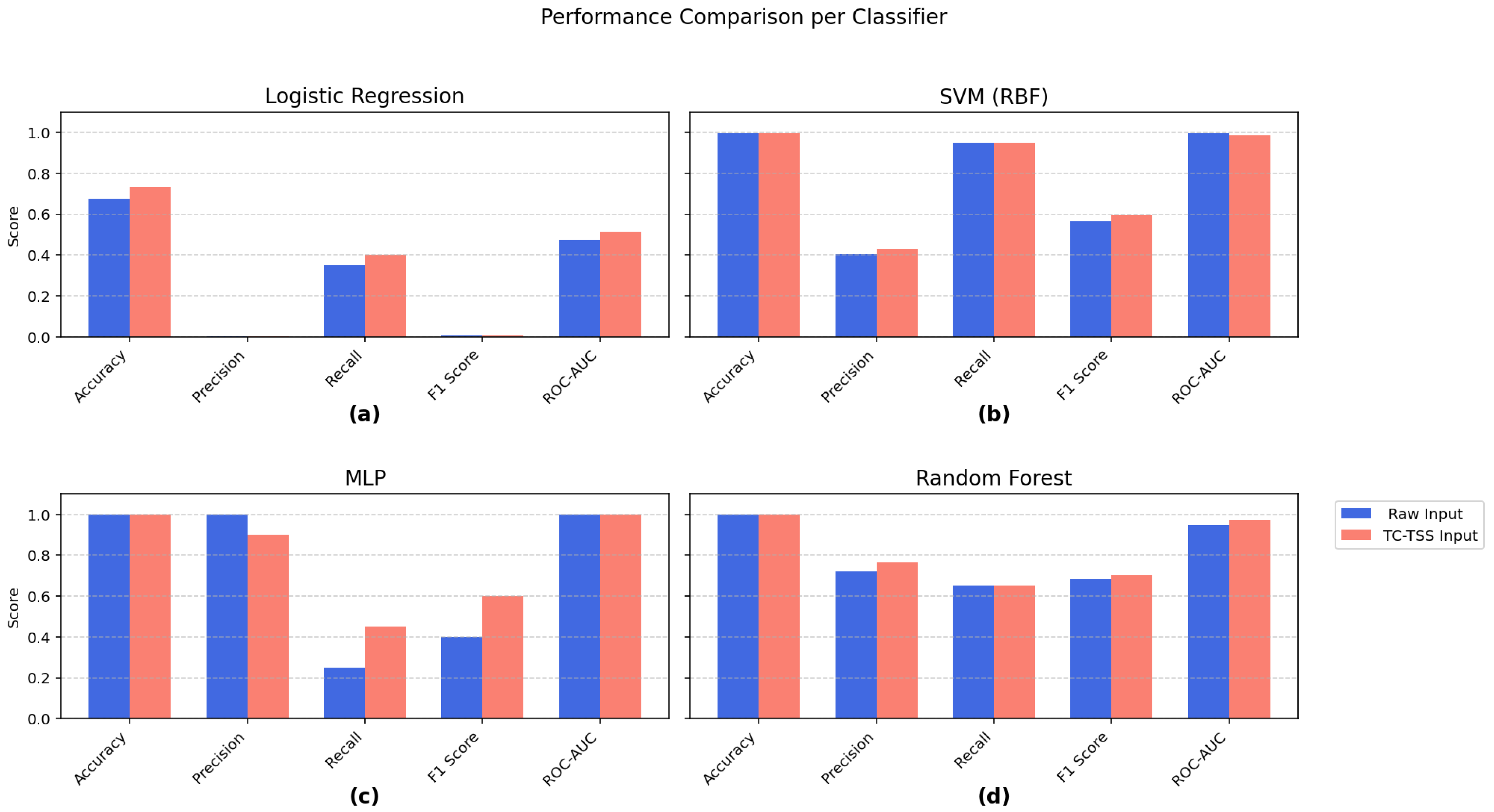
Figure 5a–d present the evaluation metrics for the four classifiers: (a) Logistic Regression, (b) SVM (RBF), (c) Multi-Layer Perceptron (MLP), and (d) Random Forest. For each classifier, five key metrics—accuracy, precision, recall, F1 score, and ROC-AUC—are reported for two input types: the original 60-s raw input windows (blue) and the TC-TSS-generated embeddings (pink).

Across all models, the TC-TSS representations (pink bars) consistently outperform the raw input features. The improvement is particularly notable in nonlinear classifiers such as MLP and Random Forest, where both F1 score and ROC-AUC show clear gains. For example, the MLP achieves AUC values approaching 0.98 and substantially higher recall and F1 score compared with the same model trained on raw features. In contrast, Logistic Regression, being a linear model, exhibits limited improvement, highlighting that the TC-TSS embeddings yield the greatest benefit when combined with nonlinear decision boundaries.

The strength of the proposed TC-TSS framework lies in its ability to capture temporal invariants within grid frequency dynamics—patterns often missed by conventional handcrafted features. Through contrastive optimisation, the encoder learns embeddings that are both invariant and discriminative, allowing for nonlinear classifiers such as SVM and MLP to form clearer decision boundaries and achieve superior AUC and F1 scores. Applied to six months of UK National Grid data, the TC-TSS-based model accurately distinguishes between stable and disturbed operating regimes, detecting frequency deviations within the statutory 49.8–50.2 Hz range with minimal false alarms. Although the performance gains are moderate, they remain meaningful given the data imbalance and limited labelled events, establishing TC-TSS as a label-efficient, physics-consistent, and scalable solution for intelligent disturbance detection in modern smart grids.

5. Discussion

This study demonstrates the effectiveness of Temporal Contrastive Self-Supervised Learning (TC-TSS) for capturing informative representations from high-resolution grid frequency data. By employing unlabelled 60-s rolling window segments, the TC-TSS framework learns task-agnostic embeddings that significantly improve the classification of frequency disturbances.

The results show clear performance gains across multiple classifiers—particularly nonlinear models such as SVM, MLP, and Random Forest—when trained on TC-TSS embeddings compared with raw time series inputs. In ROC analysis (Figure 4), both SVM and MLP achieved AUC scores of approximately 0.98–0.99, indicating excellent separability between normal and disturbance events. This is reinforced by the metric comparison (Figure 5), where improvements in recall and F1-score highlight enhanced detection of rare but critical disturbances. These outcomes confirm that contrastive learning can effectively encode temporal dependencies in power system frequency data without requiring explicit labels. The use of diverse augmentations—such as noise injection, time warping, and segment permutation—further enabled the encoder to learn generalisable patterns that capture subtle deviations in frequency behaviour.

The physical separability of latent clusters, as visualised through UMAP and t-SNE, confirms that TC-TSS learns representations aligned with actual grid dynamics. The dense clusters correspond to stable operating conditions, while boundary regions represent transient and disturbed states, validating the physical interpretability of the learned features. Once trained, the encoder can be reused across datasets or system regions, enabling scalable and transferable grid monitoring frameworks. This property makes the approach particularly valuable for integration into real-time stability assessment or early warning systems in data-scarce or evolving infrastructures.

This case study represents the first application of the TC-TSS framework to real UK National Grid frequency data. The proposed approach autonomously adapts to evolving grid dynamics and detects disturbances with high precision, eliminating the need for manual feature engineering or labelled data. Scientifically, it bridges the gap between self-supervised representation learning and power system dynamics by demonstrating that contrastively learned embeddings preserve physical invariants linked to system inertia and damping. Together, these outcomes establish a label-efficient, scalable, and physics-consistent foundation for intelligent grid analytics in low-inertia, renewable-rich power systems.

Limitations: Certain limitations remain. Linear models such as Logistic Regression showed limited benefit from the learned embeddings, suggesting that higher-capacity classifiers are required to fully exploit TC-TSS features. Additionally, the framework was validated primarily for operational limit violations; its performance on other anomaly types—such as equipment faults, load spikes, or cyber–physical disturbances—remains to be evaluated.

Future Work: Building on these findings, future research will extend the proposed TC-TSS framework in several directions. First, model generalisability will be evaluated across a broader set of grid anomalies to test applicability beyond frequency deviations. Second, advanced imbalance-handling techniques—such as sequence-aware oversampling and temporal generative models—will be explored to enhance minority-class representation while preserving temporal structure. Third, robustness under noisy or incomplete sensor data will be assessed through controlled noise injection and uncertainty quantification. Finally, adaptive fine-tuning and transfer learning across different grid regions will be investigated to validate scalability and cross-domain deployment potential.

Overall, the proposed pipeline provides a practical and effective route to frequency disturbance detection, combining self-supervised learning, interpretable classifiers, and large-scale operational data. The findings emphasise the value of contrastive representation learning in energy analytics and establish TC-TSS as a promising framework for next-generation smart grid stability monitoring.

References

1. National Energy System Operator (NESO). Operability Strategy Report; National Energy System Operator: London, UK, 2022. [Google Scholar]
2. Pollitt, M.G. Lessons from the history of independent system operators in the energy sector. Energy Policy 2012, 47, 32–48. [Google Scholar] [CrossRef]
3. Ford, R.; Hardy, J. Are we seeing clearly? The need for aligned vision and supporting strategies to deliver net-zero electricity systems. Energy Policy 2020, 147, 111902. [Google Scholar] [CrossRef] [PubMed]
4. Shrestha, A.; Gonzalez-Longatt, F. Frequency stability issues and research opportunities in converter dominated power system. Energies 2021, 14, 4184. [Google Scholar] [CrossRef]
5. Wang, Q.; Li, F.; Tang, Y.; Xu, Y. Integrating model-driven and data-driven methods for power system frequency stability assessment and control. IEEE Trans. Power Syst. 2019, 34, 4557–4568. [Google Scholar] [CrossRef]
6. Dey, M.; Rana, S.P.; Simmons, C.V.; Dudley, S. Solar farm voltage anomaly detection using high-resolution μPMU data-driven unsupervised machine learning. Appl. Energy 2021, 303, 117656. [Google Scholar] [CrossRef]
7. Dey, M.; Rana, S.P.; Wylie, J.; Simmons, C.V.; Dudley, S. Detecting power grid frequency events from μPMU voltage phasordata using machine learning. IET Conf. Proc. 2022, 2022, 125–129. [Google Scholar] [CrossRef]
8. Jeffrey, N.; Tan, Q.; Villar, J.R. A review of anomaly detection strategies to detect threats to cyber-physical systems. Electronics 2023, 12, 3283. [Google Scholar] [CrossRef]
9. Tapia, E.A.; Colomé, D.G.; Rueda Torres, J.L. Recurrent convolutional neural network-based assessment of power system transient stability and short-term voltage stability. Energies 2022, 15, 9240. [Google Scholar] [CrossRef]
10. Su, L.; Zuo, X.; Li, R.; Wang, X.; Zhao, H.; Huang, B. A systematic review for transformer-based long-term series forecasting. Artif. Intell. Rev. 2025, 58, 80. [Google Scholar] [CrossRef]
11. Dey, M.; Rana, S.P.; Dudley, S. Automated terminal unit performance analysis employing x-RBF neural network and associated energy optimisation—A case study based approach. Appl. Energy 2021, 298, 117103. [Google Scholar] [CrossRef]
12. Jung, M.; Kim, D.Y. Pseudo-labeling and time-series data analysis model for device status diagnostics in smart agriculture. Appl. Sci. 2024, 14, 10371. [Google Scholar] [CrossRef]
13. Minh, N.Q.; Khiem, N.T.; Giang, V.H. Fault classification and localization in power transmission line based on machine learning and combined CNN-LSTM models. Energy Rep. 2024, 12, 5610–5622. [Google Scholar] [CrossRef]
14. Boucetta, L.N.; Amrane, Y.; Chouder, A.; Arezki, S.; Kichou, S. Enhanced forecasting accuracy of a grid-connected photovoltaic power plant: A novel approach using hybrid variational mode decomposition and a CNN-LSTM model. Energies 2024, 17, 1781. [Google Scholar] [CrossRef]
15. Yu, P.; Cai, Z.; Zhang, H.; Cui, D.; Zhou, H.; Yu, R.; Zhou, Y. Prediction of Uncertainty Ramping Demand in New Power Systems Based on a CNN-LSTM Hybrid Neural Network. Processes 2025, 13, 2088. [Google Scholar] [CrossRef]
16. Chollet, F. Deep Learning mit Python und Keras: Das Praxis-Handbuch vom Entwickler der Keras-Bibliothek; MITP-Verlags GmbH & Co. KG: Frechen, Germany, 2018. [Google Scholar]
17. Majeed, M.A.; Phichaisawat, S.; Asghar, F.; Hussan, U. Data-Driven Optimized Load Forecasting: An LSTM Based RNN Approach for Smart Grids. IEEE Access 2025, 13, 99018–99031. [Google Scholar] [CrossRef]
18. Wang, Q.; Zhang, C.; Lü, Y.; Yu, Z.; Tang, Y. Data inheritance–based updating method and its application in transient frequency prediction for a power system. Int. Trans. Electr. Energy Syst. 2019, 29, e12022. [Google Scholar] [CrossRef]
19. Ericsson, L.; Gouk, H.; Loy, C.C.; Hospedales, T.M. Self-supervised representation learning: Introduction, advances, and challenges. IEEE Signal Process. Mag. 2022, 39, 42–62. [Google Scholar] [CrossRef]
20. Goyal, P.; Mahajan, D.; Gupta, A.; Misra, I. Scaling and benchmarking self-supervised visual representation learning. In Proceedings of the IEEE/CVF International Conference on Computer Vision, Seoul, Republic of Korea, 27 October–2 November 2019; pp. 6391–6400. [Google Scholar]
21. Georgescu, M.I.; Barbalau, A.; Ionescu, R.T.; Khan, F.S.; Popescu, M.; Shah, M. Anomaly detection in video via self-supervised and multi-task learning. In Proceedings of the IEEE/CVF Conference on Computer Vision and Pattern Recognition, Nashville, TN, USA, 19–25 June 2021; pp. 12742–12752. [Google Scholar]
22. Fei, K.; Li, Q.; Zhu, C.; Dong, M.; Li, Y. Electricity frauds detection in Low-voltage networks with contrastive predictive coding. Int. J. Electr. Power Energy Syst. 2022, 137, 107715. [Google Scholar] [CrossRef]
23. Liu, X.; Liu, X.; Dou, J.; Zhu, Z.; Wang, J. A Virtual Measurement Method of Industrial Power Consumption Scenario Based on Self-Supervised Contrast Learning. In Proceedings of the 2025 10th Asia Conference on Power and Electrical Engineering (ACPEE), Beijing, China, 15–19 April 2025; pp. 1151–1155. [Google Scholar]
24. Eldele, E.; Ragab, M.; Chen, Z.; Wu, M.; Kwoh, C.K.; Li, X.; Guan, C. Self-supervised contrastive representation learning for semi-supervised time-series classification. IEEE Trans. Pattern Anal. Mach. Intell. 2023, 45, 15604–15618. [Google Scholar] [CrossRef]
25. Wang, X.; Jiao, S.; Chen, Q. Voltage Prediction of Lithium-Ion Battery Based on Time Contrastive Learning Model. Energy Technol. 2025, 13, 2401854. [Google Scholar] [CrossRef]
26. Jeong, J.; Ku, T.Y.; Park, W.K. Denoising masked autoencoder-based missing imputation within constrained environments for electric load data. Energies 2023, 16, 7933. [Google Scholar] [CrossRef]
27. Dong, Z.; Hou, K.; Liu, Z.; Yu, X.; Jia, H.; Tang, P.; Pei, W. A fast reliability assessment method for power system using self-supervised learning and feature reconstruction. Energy Rep. 2023, 9, 980–986. [Google Scholar] [CrossRef]
28. Uelwer, T.; Robine, J.; Wagner, S.S.; Höftmann, M.; Upschulte, E.; Konietzny, S.; Behrendt, M.; Harmeling, S. A survey on self-supervised methods for visual representation learning. Mach. Learn. 2025, 114, 1–56. [Google Scholar] [CrossRef]
29. Gong, X.; Wei, Y.; Du, W.; Gao, Y.; Guan, T. Self-supervised contrastive learning with time-frequency consistency for few-shot bearing fault diagnosis. Meas. Sci. Technol. 2025, 36, 066204. [Google Scholar] [CrossRef]
30. Liu, D.; Wang, T.; Liu, S.; Wang, R.; Yao, S.; Abdelzaher, T. Contrastive self-supervised representation learning for sensing signals from the time-frequency perspective. In Proceedings of the 2021 International Conference on Computer Communications and Networks (ICCCN), Athens, Greece, 19–22 July 2021; pp. 1–10. [Google Scholar]
31. Liu, Y.; Wang, K.; Liu, L.; Lan, H.; Lin, L. Tcgl: Temporal contrastive graph for self-supervised video representation learning. IEEE Trans. Image Process. 2022, 31, 1978–1993. [Google Scholar] [CrossRef]
32. Ding, Y.; Zhuang, J.; Ding, P.; Jia, M. Self-supervised pretraining via contrast learning for intelligent incipient fault detection of bearings. Reliab. Eng. Syst. Saf. 2022, 218, 108126. [Google Scholar] [CrossRef]
33. Maitreyee, D.; Rana, S.P. High-Resolution Electrical Measurement Data Processing. G.B. Patent Application No. GB2016025.5A, 21 December 2022. [Google Scholar]
34. Ross, B.A.; Chen, Y.; Liu, Y.; Kim, J. Challenges, Industry Practice, and Research Opportunities for Protection of IBR-Rich Systems; Pacific Northwest National Laboratory (PNNL): Richland, WA, USA, 2024.
35. Radhoush, S.; Whitaker, B.M.; Nehrir, H. An overview of supervised machine learning approaches for applications in active distribution networks. Energies 2023, 16, 5972. [Google Scholar] [CrossRef]
36. National Grid ESO. Frequency Data Portal. 2025. Available online: https://www.nationalgrideso.com/data-portal/frequency-data (accessed on 4 June 2025).
Figure 1. System frequency measurements for Great Britain recorded at 1-s intervals throughout June 2025.
Energies 18 05611 g001
Figure 2. Pipeline of the proposed TC-TSS method used to capture contrastive patterns for evaluating classification models.
Energies 18 05611 g002
Figure 3. Embedding visualisations representing high-dimensional learned features from time series frequency data, also highlighting potential outliers. The diagram compares (a) UMAP and (b) t-SNE, illustrating the differences in preserving global versus local structure.
Energies 18 05611 g003
Figure 4. Receiver operating characteristic (ROC) comparison of all evaluated classification models using (a) raw rolling window input features and (b) TC-TSS-extracted embeddings as input.
Energies 18 05611 g004
Figure 5. Statistical metric-based performance comparison of raw rolling window input and TC-TSS-extracted input across all evaluated classifiers: (a) Logistic Regression, (b) SVM with RBF kernel, (c) MLP, and (d) Random Forest.
Energies 18 05611 g005