Abstract
To address the high costs and inefficiencies of blind prospecting in deep geothermal exploration, this study develops a three-dimensional heat transfer model for quantitative prediction of geothermal enrichment targets. Unlike traditional qualitative or single-mechanism analyses, this research utilizes a finite element forward modeling approach based on step-faulted depressions (sedimentary basins/grabens) and uplifts (domes/uplift belts). We simulate temperature fields and heat flux distributions in multilayered systems incorporating four thermal conductivity types (A, K, H, Q). By systematically comparing the geometric heat flow convergence in depressions with the lateral diffusion in uplifts, this work reveals mirror and anti-mirror relationships between temperature fields and structural morphology at middle and deep levels, as well as local “hot spot” and “cold zone” effects. The results indicate that, in depressional structures, shallow high-temperature reservoirs (<2 km) are mainly concentrated in A- and K-types, while deeper reservoirs (>3 km) are enriched in Q- and H-types. In contrast, uplift structures are characterized by mid- to shallow-depth (<3 km) reservoirs predominantly in A- and K-types, with high temperatures at depth preferentially hosted in A- and H-types, and the highest temperatures observed in the A-type. Thermal conductivity contrasts, layer thicknesses, and structural morphology collectively control the spatial distribution of heat flux. A strong positive correlation between thermal conductivity and heat flux is observed at the central target area, significantly stronger than at the margins, whereas this relationship is notably weakened in Q-type. Crucially, low-conductivity zones display high geothermal gradients coupled with low terrestrial heat flow, disproving the axiom that “elevated geothermal gradients imply high heat flow,” thus establishing “high-gradient/low-heat-flow coupling zones” as strategic exploration targets. The model developed in this study demonstrates high simulation accuracy and computational efficiency. The findings provide a robust theoretical basis for reconstructing geothermal geological evolution and precise geothermal target localization, thereby reducing the risk of “blind heat exploration” and promoting the cost-effective and refined development of deep concealed geothermal resources.
1. Introduction
Geothermal energy, as a renewable and non-polluting clean energy source [1,2,3,4], can effectively supplement the fossil fuel energy system [5,6]. Unlike tidal, wind, and solar energy-which are dependent on meteorological conditions-geothermal resources possess virtually unlimited sustainability and are independent of climate [7,8,9,10]. At present, extensive deep geothermal exploration and development has been conducted internationally [11], whereas large-scale development in China has yet to be realized. The primary limitations lie in the high cost of exploration and development, unclear formation mechanisms of deep thermal reservoirs, and particularly the lack of high-quality, highly exploitable “geothermal sweet spots”—that is, reservoirs characterized by shallow burial depth and high temperatures. Currently, geothermal development in China remains focused on “geothermal sweet spots” such as hot springs, and has not overcome the challenge of exploring areas with no evident surface heat anomalies [12,13,14]. This makes it difficult to achieve the goal of “exploring for heat where none is apparent”. Therefore, advancing methodologies for predicting favorable geothermal zones is of significant scientific and practical value for reducing exploration risk and achieving precise resource targeting. There is an urgent need to deepen research into geothermal field genesis models and optimize techno-economic strategies.
Many scholars have conducted extensive research on the formation of high geothermal anomaly zones within geothermal fields [15,16,17,18,19]. Multi-scale studies indicate that the main controlling factors of geothermal anomalies can be summarized into three categories: (a) Heat source mechanisms: deep heat input mainly originates from mantle heat flow, radiogenic heat production, and magmatic activity [20,21]. Magma chambers can provide a sustained heat source [22], and Cenozoic magmatism shows a significant correlation with heat flow [23]. (b) Heat transfer mechanisms: fault systems serve as dominant channels for heat transport, with enhanced deep high-temperature fluid convection promoting ground temperature increases [24,25,26,27]. Gao et al. [28] further found that convective heat transfer processes involving mass exchange are necessary for raising subsurface temperatures. (c) Heat redistribution mechanisms: basement undulations and caprock thickness significantly influence the spatial distribution of the geothermal field through the thermal refraction effect. Specifically, uplifted basement areas with high thermal conductivity are prone to forming positive temperature anomalies, and heat flow is positively correlated with basement relief, reflecting a focusing effect of heat flow migration toward regions of low thermal resistance [19,29].
The formation of geothermal fields is governed by the coupling of multiple factors, with the central challenge being the identification of the dominant controlling elements and the construction of the predictive models for favorable geothermal zones [30,31]. This study investigates how structural morphology (depressions/uplifts) and layered thermal conductivity jointly control heat enrichment, providing a systematic, comparative analysis to elucidate the governing patterns and mechanisms. We develop and validate a high-accuracy, high-efficiency three-dimensional forward heat-transfer model that quantitatively predicts deep geothermal enrichment patterns and field characteristics, thereby reducing the costs and uncertainties of blind deep exploration. By constructing a three-dimensional heat transfer numerical model, this research quantitatively investigates the differentiation of temperature fields governed by coupled structural morphology and thermal conductivity stratification. The model quantitatively characterizes the spatial distribution patterns of typical geological units (sedimentary basins and dome/uplift areas) and reveals the heat flow convergence and enrichment in the low-lying parts of depressions, as well as the migration mechanisms of thermal disturbances in the elevated sections of uplifts—thus overcoming the limitations of traditional qualitative analyses. The results demonstrate that depressional structures tend to guide heat flow, forming target zones for resource enrichment, while uplifted structures govern the transmission paths of thermal disturbances; together, they jointly control the spatial differentiation patterns of the geothermal field. This model provides a physical and theoretical foundation for reconstructing geological evolution and quantitatively predicting exploration targets. It offers significant practical value for reducing the technical risks associated with “blind” geothermal exploration and achieving precise, cost-effective delineation of geothermal resources. Ultimately, it supports the expansion of geothermal development from traditional hot spring and surface anomaly zones to deeply buried, concealed resources.
2. Methodology
2.1. Heat Transfer Model
This study establishes a 3D heat transfer model for depression-type and uplift-type geological structures (Figure 1), the parameters for each stratum are listed in Table 1, aiming to quantitatively simulate the spatial distribution characteristics of geothermal mass transfer processes and resource enrichment patterns under different tectonic settings. These two model highly abstract the structural features of typical geological units—such as sedimentary basins/fault-depression zones (depression-type) and dome areas/uplift belts (uplift-type)—thereby establishing mathematical and physical foundations for unraveling the mechanisms of geological environment evolution and resource distribution.
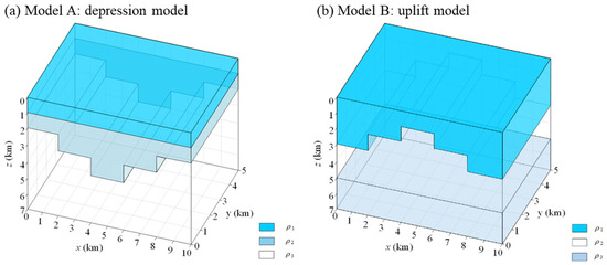
Figure 1.
Three-dimensional models of depressional and uplifted geological structures.

Table 1.
Thermal conductivity of uplift and depression models.
Depression-type structures characterize sedimentary convergence zones in crustal extensional environments. The model comprises an overlying layer (ρ1), an intermediate layer (ρ2), and a basal layer (ρ3). Its strata exhibit stepped subsidence, forming a pronounced central depression basin that facilitates sediment accumulation, heat concentration, and fluid enrichment. These zones typically evolve into efficient reservoirs for geothermal energy, hydrocarbons, and groundwater resources. Uplift-type structures reflect crustal compression or tectonic uplift forces. Their strata demonstrate stepped uplift morphology with a central protrusion and peripheral downwarping. This configuration promotes vertical diffusion and lateral dissipation of heat flow, regulating shallow geothermal energy release and restoring thermal equilibrium within strata.
The two models scientifically reconstruct the spatial distribution patterns of geological units—including sedimentary basins/fault-depression zones (depression-type) and dome areas/uplift belts (uplift-type)—through stepped interfacial variations. Depression structures highlight the resource enrichment effects in depressed zones, while uplift structures reveal the heat flow perturbation mechanisms in elevated sections, collectively providing a theoretical foundation for geothermal resource exploration and development.
2.2. Governing Equation
Consider a homogeneous half-space (semi-infinite medium) as the study domain and embed within it an anomalous body with contrasting thermal conductivity. The differential form of the heat conduction governing equation for the underground space can be expressed as [32,33,34]:
Impose the following boundary conditions: the top boundary is held at a constant temperature Tup, the lateral boundaries are adiabatic (insulated), and the bottom boundary has a prescribed heat flux qdown. Given the thermal conductivity distribution and these boundary conditions, use finite-element simulation to compute the three-dimensional subsurface temperature field. The boundary conditions are set as follows [35,36]:
The temperature at the upper boundary is set to a constant value Tup:
where T represents the temperature.
In three-dimensional space, the adiabatic boundary conditions on the four surrounding side surfaces can be expressed as:
where n is the unit normal vector to the boundary.
The heat flux condition at the lower boundary can be expressed as:
where k is the thermal conductivity, and qdown is the heat flux value.
2.3. Finite-Element Analysis
In this study, a hexahedral mesh discretization is used for finite element numerical simulation of the temperature field. Within each hexahedral element, both the temperature T and the thermal conductivity k are linearly interpolated [37,38]:
where i denotes the node index, Ti represents the temperature at each node of the element (in °C), ki denotes the thermal conductivity at each node of the element, and Ni is the shape function, as defined in Equation (7) [39]:
where (, , ) is the position of the ith node in the local coordinate system. The local coordinates are written as follows:
where x0, y0, and z0 are the center of the sub-element along the x-, y-, and z-directions, respectively, and a, b, and c are the length, width, and height, respectively.
The partial differential Equation (1) is multiplied by a test (weighting) function δT and integrated as follows:
According to the computation rules of the Hamilton operator in field theory [17], substituting the boundary conditions into Equation (9), the integral equation for heat conduction of the underground space temperature field can be obtained as follows:
where is the study region, is the upper boundary, is the lower boundary, qdown is the heat flux value, k is the thermal conductivity, T is the temperature, denotes the divergence operator, represents the gradient operator, and is the test (weighting) function.
By discretizing and linearly interpolating the integral form of the heat conduction equation for the underground space temperature field, the element integrals for each term in the integral equation can be obtained:
where δTe is the array of test (weighting) functions within the element, Te is the temperature array within the element, K1e and K2e are the stiffness matrices within the element, and P1e and P2e are the source vectors within the element. The coefficients in the stiffness matrices and source vectors can be obtained as follows:
where k1ij, k2ij, p1ij, and p2ij represent the elements in the stiffness matrices K1e, K2e and the source vectors P1e, P2e, respectively, i, j, and l denote node indices, a, b, and c are the side lengths of the sub-element in the x-, y-, and z-directions, k is the thermal conductivity; , , are the coordinates of node i in the parent element; Tup denotes the upper boundary temperature; and qdown denotes the bottom boundary heat flux.
Based on the numbering of each unit and node, by expanding to the positions of elements corresponding to the research area, the linear system of equations for the assembled global stiffness matrix and source vector can be obtained:
where δT denotes the impulse function array, T is the temperature field array, K1 and K2 represent the stiffness matrices, and P1 and P2 represent the source vectors.
Equation (19) can be simplified as:
where K = K1 + K2, and P = P1 + P2
By solving this system of linear equations, the three-dimensional temperature field distribution of the underground space can be obtained.
3. Results
3.1. Model Verification
To evaluate the stability and accuracy of the algorithm developed in this study, we conducted a comparative analysis against the commercial software COMSOL Multiphysics 5.6. Under identical model configurations and parameter settings, three-dimensional (3D) temperature fields were computed using both the proposed algorithm and COMSOL Multiphysics. In terms of mesh configuration, this study uses a hexahedral mesh, while COMSOL employs a tetrahedral mesh. Regardless of the scheme, computational accuracy varies with mesh scale: finer meshes yield higher accuracy but significantly increase computational cost. Balancing accuracy and efficiency at the geothermal-field scale, a mesh size of 100–200 m is appropriate. Thus, this study adopts mesh spacings of 200 m × 200 m × 100 m in the x, y, and z directions, respectively. Temperature–depth profiles were then extracted at three representative locations (CX1 (1, 3, 0), CX2 (3, 3, 0), and CX3 (5, 3, 0)) for comparative analysis, and the goodness-of-fit between the two results was quantified. As shown in Figure 2, for both the depression and uplift models, the goodness-of-fit at CX1, CX2, and CX3 exceeds 99%, thereby indicating that the proposed algorithm is suitable for heat-transfer modeling and analysis.
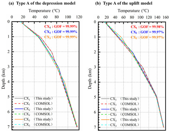
Figure 2.
Comparison between the proposed algorithm and COMSOL simulation results.
3.2. Thermal-State Characteristics of a Depression Model Under Different Modes
3.2.1. Horizontal Distributions of the Temperature Field Under Different Modes in a Depression Model
Figure 3 displays the temperature field distribution of a depression model under varying thermal conductivity distributions. Overall, the temperature field is markedly controlled by formation thermal conductivity. Even with identical geological structures, different combinations of thermal conductivity parameters lead to significant differences in temperature gradients and isothermal surface morphology. Near formation interfaces, temperature contours frequently exhibit bending or local clustering, demonstrating a strong layer-controlled effect. This response is particularly pronounced at interfaces with abrupt thermal conductivity changes between layers. The temperature field does not vary uniformly; instead, abrupt shifts in interlayer thermal conductivity and variations in formation thickness collectively govern the detailed distribution patterns of local temperature fields.
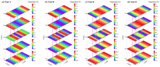
Figure 3.
Three-dimensional temperature fields of the depression model for types A, K, H, and Q.
The diverse thermal conductivity models (Type A, K, H, and Q) induce distinct temperature field responses. In Type A, where the overlying layer exhibits the lowest thermal conductivity while middle and underlying layers progressively increase, heat transfer becomes impeded in the upper section. This results in a diminishing temperature gradient from top to bottom, with high temperatures and significant variations in the upper part and reduced thermal contrast in the lower zone. Type K features the highest conductivity in the middle layer, creating a “high-speed thermal conduit”. Here, temperature contours flatten in the middle stratum with minimal variation but exhibit pronounced bending at interfaces between the middle and adjacent layers. Type H displays maximum conductivity at the top and minimum in the middle, forming a “thermal barrier” that obstructs heat flow in the central layer. This causes localized steep temperature gradients and heat accumulation. Lastly, Type Q shows monotonically decreasing thermal conductivity downward, concentrating heat in the low-conductivity basal layer. Consequently, high-temperature zones develop at depth with densely clustered contours.
The impact of thermal conductivity on temperature fields manifests primarily in two aspects: First, in high-conductivity formations, heat flows readily through, resulting in smaller temperature gradients and reduced thermal contrast. Conversely, in low-conductivity strata, heat transfer is impeded, leading to heat accumulation and consequently larger temperature gradients and temperature anomalies. Second, abrupt changes in thermal conductivity across layer interfaces directly alter heat flow pathways, causing temperature field structures to bend and form localized anomalies at boundaries. When conductivity shifts abruptly from high to low, contours become densely clustered, indicating obstructed heat flow and amplified temperature differentials. This dual mechanism—stratigraphic conductivity gradients controlling heat diffusion patterns, and interfacial discontinuities distorting thermal distributions—underpins the distinct responses observed across different conductivity models.
The temperature field differences described above primarily stem from three aspects: Firstly, the stratigraphic sequence effect of thermal conductivity governs the efficiency of heat transfer along the depth direction. A “low-high” configuration (low conductivity in upper layers, high in lower) causes heat to accumulate predominantly in the upper strata, while a “high-low” arrangement (high conductivity in upper layers, low in lower) facilitates higher temperatures in deeper zones. Secondly, the thermal conductivity of intermediate layers often acts as either a “barrier” or a “conduit,” significantly impacting heat transfer and temperature distribution between upper and lower strata. Thirdly, sharp thermal conductivity contrasts at stratigraphic interfaces tend to generate distinct temperature accumulation zones or rapid transition bands, creating localized hotspots or cold spots.
In summary, the spatial distribution of the temperature field in the depression model is chiefly controlled by both the absolute thermal conductivity values of each layer and their vertical arrangement. Whether low-conductivity layers are positioned in upper or lower sections, they readily trigger significant localized temperature anomalies. Meanwhile, the thermal conductivity of intermediate layers critically regulates heat exchange efficiency between upper and lower strata, playing a decisive role in governing overall heat flux as well as the intensity and spatial distribution of temperature anomalies.
3.2.2. Vertical Distributions of the Temperature Field Under Different Modes in a Depression Model
Figure 4 displays vertical temperature field slices at the central section (y = 2.5 km) of the depression model under different stratigraphic thermal conductivity combinations. The four slices in Figure 4 correspond to Type-A, Type-K, Type-H, and Type-Q conductivity configurations. Under these varying thermal conductivity arrangements, distinct differences emerge in the distribution, density, and curvature characteristics of the temperature contours. Overall, the temperature field exhibits significant interlayer differentiation. At stratigraphic interfaces and within the central depression zone, the temperature contours display complex morphologies, reflecting heterogeneous coupling effects between the geometric structure of the formations and their thermal properties. Variations in thermal conductivity influence both the rate of heat flow propagation and the locations of thermal accumulation, thereby governing the formation patterns of temperature anomaly zones and hotspots.
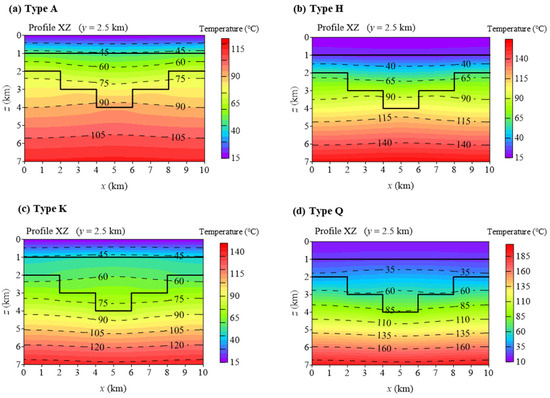
Figure 4.
Temperature field on a central vertical cross-section (y = 2.5 km) of the depression model.
For Type A, the overlying layer has the lowest thermal conductivity, with progressively higher values in the intermediate and underlying layers. Upward heat propagation is impeded, leading to heat accumulation. This results in steep temperature gradients, elevated temperatures, and dense temperature contours in the top layer, indicating shallow heat concentration. While heat readily penetrates the high-conductivity lower sections, the uniform temperature distribution shows minimal thermal contrast at depth—though overall temperatures remain relatively low in deeper strata. The central depression zone exhibits contours bending inward downward, revealing structural redistribution of heat flow.
For Type K, the intermediate layer shows maximum thermal conductivity, functioning as a high-efficiency thermal conduit. Heat rapidly traversing this layer significantly reduces heat descent rates and flattens temperature gradients, manifesting as sparse and linear contours in this interval. Conversely, contour bending and concentration occur at layer interfaces. This configuration facilitates distinct high-temperature zones in both upper and lower layers, with the intermediate layer dominating temperature anomalies in the central depression.
For Type H, thermal conductivity peaks in the top layer, hits minimum in the intermediate layer, and shows moderate values in the base layer. Heat penetrates the top layer rapidly but accumulates at the low-conductivity intermediate layer, causing sharp temperature spikes, ultra-dense contours, and formation of a thermal barrier zone. Heat dissipation in the bottom layer gradually moderates temperature gradients, while the central depression develops localized hotspots due to this energy trapping.
For Type Q, thermal conductivity decreases progressively from top (highest) to bottom (lowest). Downward heat transfer efficiency reduces correspondingly: heat rapidly exits the top layer, transfers moderately through the middle section, and accumulates heavily in the ultra-low-conductivity base layer. This creates extreme temperatures, with the densest contours concentrated at the depression bottom and underlying low-conductivity strata. The resulting energy density establishes the depression’s lower section as the optimal thermal storage target.
The fundamental control mechanism underlying the similarities and differences in the temperature field lies in the regulation of heat flow conduction and temperature distribution by variations in formation thermal conductivity and interlayer abrupt changes. In regions of high thermal conductivity, heat flows smoothly with small temperature gradients and minimal differentials; conversely, areas of low thermal conductivity tend to form “thermal accumulation” phenomena with pronounced temperature discontinuities. Particularly at interfaces where interlayer thermal conductivity changes abruptly, temperature isotherms readily concentrate or become discontinuous. Localized thickening induced by the geometric configuration of depressions further causes heat flow to accumulate or dissipate within these concave structures, thereby intensifying the stratigraphic control and zonal response of the temperature field. The vertical sequencing of different thermal conductivities ultimately shapes the longitudinal distribution pattern of thermal energy throughout the entire stratum system.
Therefore, we can derive geological guidance for efficient geothermal exploration from the depressions model:
(1) Prioritize exploring below low-thermal-conductivity insulating layers: Beneath low-conductivity basal formations—whether Q-type or H-type—regions often develop “thermal reservoir capsules” (high-temperature zones), making them preferred targets.
(2) Leverage intermediate layers’ “thermal barrier/channel” effects: Intermediate layers with sharp conductivity contrasts can block or redirect thermal energy. Areas beneath thermal barriers (especially thick depression sections with low-to-medium conductivity) frequently host high-quality geothermal reservoirs.
(3) Integrate structural and thermal property analysis: Temperature anomalies typically coincide with thick depression sections and low-thermal-conductivity formations. Prioritizing well placement in these belt-shaped zones significantly enhances exploration efficiency.
(4) Optimize parameters through comparative cross-layer experiments: Actual geothermal surveys should incorporate formation-specific conductivity tests, selecting Q-type or H-type analogs to maximize temperature and energy accumulation potential.
In summary, the temperature-field distribution in depression models reflects both geometric structural controls and layered thermal-conductivity configurations. Understanding temperature-field responses under varying structural-thermal modes provides critical guidance for efficient geothermal resource development and scientific site selection.
3.2.3. Thermal Conductivity–Temperature Field Correlation Analysis in a Depression Model
Figure 5 illustrates the variations in temperature (red curve) and thermal conductivity (blue curve) with depth. Overall, the thermal conductivity exhibits a three-segment distribution, corresponding to the thermal properties (ρ1, ρ2, ρ3) of rock layers at different depths. The blue curve shows abrupt changes at each interface, forming a step-like pattern. Meanwhile, the temperature curve appears as a segmented polyline: within each layer, temperature increases progressively with depth, while the slope changes abruptly at layer interfaces. The red temperature curves in the figure vary approximately linearly with depth within each thermal-conductivity layer, reflecting a nearly constant geothermal gradient, but exhibit inflection points at layer boundaries due to abrupt changes in thermal conductivity, resulting in an overall piecewise-linear form. The degree of linearity is similar across different locations (CX1–CX3) and model types (A, H, K, Q). The main differences lie in the gradient magnitude—becoming steeper or gentler with changes in conductivity—and in the positions of the inflection points caused by variations in interface depth.
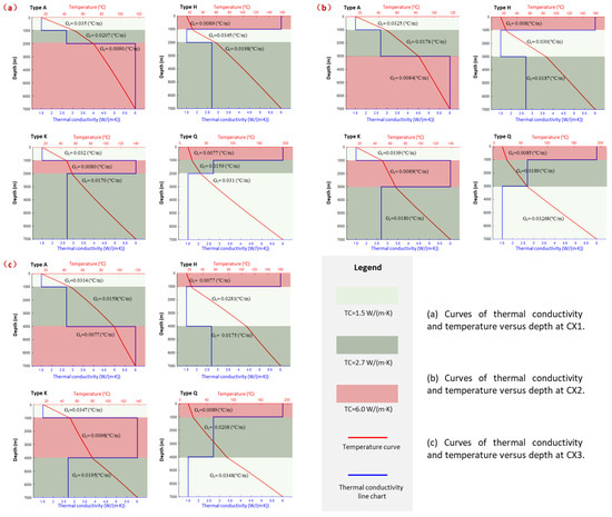
Figure 5.
Thermal conductivity and temperature distribution characteristics of the depression model under different types A, K, H, and Q.
Thermal conductivity directly influences the steepness of the temperature gradient (geothermal gradient, Gt). According to the fundamental principle of heat conduction, Gt is inversely proportional to thermal conductivity λ (Gt = q/λ, where q is heat flux density). Taking Type A as an example: In the shallow layer (0–2 km), thermal conductivity is lowest (λ = 1.5 W/(m·K)), resulting in the steepest temperature curve (red) and maximum geothermal gradient (G = 0.035 °C/m). In the middle layer, moderate thermal conductivity (λ = 2.7 W/(m·K)) leads to a gentler temperature curve (G = 0.0207 °C/m). In the deep layer, the highest thermal conductivity (λ = 6.0 W/(m·K)) substantially slows the temperature rise (G = 0.0099 °C/m). Type K resembles Type A but exhibits higher thermal conductivity in the middle layer, causing an even flatter temperature curve. For Type s H and Q, the high-conductivity layer lies in the upper section, while the bottom layer has low thermal conductivity. This configuration corresponds to a slow temperature increase at shallow depths and a sharp rise in deeper zones, reflecting the accumulated effect of thermal resistance.
Under different spatiotemporal points (CX1, CX2, CX3), even with identical model parameters, local variations in topography (e.g., convex uplifts or concave depressions), boundary conditions, and subtle differences in heat flux density can induce localized changes in temperature curves. For example, the heat accumulation effect at the base of depression zones (such as CX3) results in higher temperature values and steeper geothermal gradients at equivalent depths compared to uplifted areas. This phenomenon is particularly evident when comparing identical regions across different models. In Type A, for instance, temperature curves at CX2 and CX3 exhibit steeper gradients than at CX1, revealing a “heat sink effect” arising from the coupling of topography and heat flux conditions.
The fundamental disparities in temperature distribution primarily stem from the following aspects: (a) the absolute values and distribution sequence of thermal conductivity in each stratum, which directly dictate temperature gradients within individual lithological segments; (b) layer thickness and boundary depths, which govern cumulative temperature variations across segmented intervals; and (c) topographical features (e.g., depressions and uplifts) that redistribute heat flux density and pathways, inducing localized thermal anomalies or cold zones. Collectively, lower thermal conductivity correlates with increased geothermal gradients, accelerating temperature elevation with depth, whereas higher thermal conductivity facilitates uniform heat dissipation, thereby mitigating localized temperature rise.
Overall, the spatial distribution of stratum thermal conductivity directly governs both temperature field patterns and geothermal gradients. Highly conductive rock formations facilitate uniform heat transfer, thereby lowering geothermal gradients; conversely, low-conductivity strata impede thermal flux, leading to localized heat accumulation and accelerated temperature escalation with depth. Distinct geological types (A, H, K, Q) further regulate thermal distribution profiles through differential rock assemblages, bedding structures, and thickness configurations—type A exhibits peak shallow temperatures, while type Q demonstrates maximum deep temperatures.
In the three-layer model, the distribution of thermal conductivity directly governs the segmented slope characteristics of temperature curves. The cumulative temperature curves corresponding to different models reveal stepwise thermal resistance effects alongside localized modulation by topography and heat flow distribution. Figure 5 systematically illustrates the spatial heterogeneity inherent in coupled subsurface heat conduction processes: the interconstrained relationships among lithology, thermal conductivity, heat flux, and temperature constitute the theoretical foundation for interpreting thermal anomalies and geothermal gradient variations across distinct geological units. These distribution patterns not only elucidate the mechanistic underpinnings of spatial variability in subsurface temperature fields but also establish a robust physical basis for refined regional geothermal modeling and geothermal resource assessment.
3.3. Thermal-State Characteristics of an Uplift Model Under Different Modes
3.3.1. Horizontal Distributions of the Temperature Field Under Different Modes in an Uplift Model
Figure 6 depicts the temperature field distribution characteristics at varying depths for types A, K, H, and Q within an uplift geological framework.
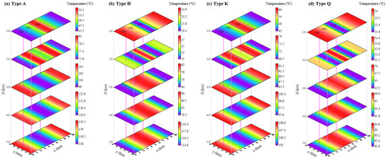
Figure 6.
Three-dimensional temperature fields of the uplift model (types A, K, H, and Q).
In type A, the uppermost low-conductivity layer (1.5 W/(m·K)) exhibits pronounced thermal insulation, limiting upward heat transfer and inducing rapid temperature accumulation at shallow depths (<1 km) with steep gradients. The intermediate layer (2.7 W/(m·K)) enhances conductive efficiency, while the high-conductivity basal layer (6.0 W/(m·K)) facilitates rapid heat dissipation. Consequently, the steepest temperature gradient occurs at shallow depths (~1 km), moderating in the intermediate zone and flattening substantially at depths >3 km due to efficient deep heat redistribution.
In type K, despite sharing an identical low-conductivity cap (1.5 W/(m·K)) with type A, the ultra-conductive intermediate layer (6.0 W/(m·K)) acts as a thermal conduit, homogenizing deep temperatures. Shallow thermal patterns resemble type A, but the gradient diminishes sharply in the intermediate layer. The basal moderate-conductivity layer (2.7 W/(m·K)) yields slightly elevated deep temperatures with enhanced horizontal uniformity compared to type A.
In type H, the conductive upper layer (6.0 W/(m·K)) enables efficient vertical heat transfer, resulting in subdued shallow gradients. A pronounced thermal barrier emerges in the ultra-low-conductivity intermediate layer (1.5 W/(m·K)), triggering an abrupt gradient increase. The basal layer (2.7 W/(m·K)) exhibits moderated warming, though warming rates exceed those in type Q. Minimal temperature fluctuations characterize shallow depths, contrasting sharply with accelerated warming in the intermediate thermal barrier.
In type Q, the conductive cap (6.0 W/(m·K)) promotes rapid heat loss, yielding the lowest shallow temperatures and minimal initial warming. Progressive warming occurs through the intermediate layer (2.7 W/(m·K)), while extreme heat accumulation in the basal low-conductivity unit (1.5 W/(m·K)) generates pronounced temperature peaks at depth. This configuration produces the shallowest minimum temperatures and the most abrupt deep thermal culmination, with maxima localized near the basal arch.
The differences in temperature fields between various models are primarily attributed to three factors: (1) Thermal Conductivity Stratigraphy Dominance: When the upper layer exhibits low thermal conductivity (e.g., types A and K), the temperature gradient increases significantly, resulting in rapid temperature rise. Conversely, high thermal conductivity in the upper layer (e.g., type Q) leads to cooler shallow regions, while low conductivity in deeper strata produces extreme high-temperature zones at depth. (2) Interlayer Relay Effects: A highly conductive middle layer (e.g., type l K) moderates the mid-deep thermal field, smoothing extreme value transitions. In contrast, a low-conductivity middle layer (e.g., type H) creates a thermal barrier zone, causing abrupt temperature changes. (3) Basal Control of Extremes: Exceptionally low thermal conductivity in the basal layer (e.g., type Q) intensifies deep thermal ascent, forming a “deep thermal island”. Conversely, high basal conductivity (e.g., type A) impedes heat accumulation at depth.
The temperature fields of uplifted and depressed models exhibit distinct characteristics at varying depths: Shallow Depths (e.g., 1 km): Uplifted models demonstrate lower temperatures than depressed models. This discrepancy stems from heat flow divergence at uplifted crests, where a “funneling effect” dissipates thermal energy, inducing crestal cooling. Conversely, depressed terrains act as heat flow convergence zones, minimizing lateral heat loss and elevating shallow temperatures. Mid-Deep Depths (e.g., 3–5 km): Depressed models develop pronounced “thermal islands,” while uplifted counterparts display smoother thermal distributions. Temperatures in depressed systems significantly exceed those in uplifted models at equivalent depths. This arises from spatial heat flow accumulation in depressed basins; when underlain by low-conductivity strata (e.g., Q-type), extreme basal hyperthermia amplifies this “island” effect. Although uplifted bases may harbor heat storage potential, pervasive heat flow dispersion suppresses peak basal temperatures, yielding gentler thermal gradients.
The temperature discrepancies among distinct thermal conductivity types intensify in depressed models. Taking Q-type as an example, low basal conductivity facilitates severe heat “accumulation” at the basin floor, resulting in markedly more intense deep thermal ascent than in uplifted equivalents. Conversely, A- and K-types exhibit opposing behaviors: high-conductivity basal layers accelerate deep heat dissipation, accentuating minimum temperature points at depth. Moreover, depressed H- and Q-type systems universally demonstrate higher shallow temperatures than their uplifted counterparts—a critical factor in geothermal resource assessment. Geothermally, uplifted models display overall arching isotherm surfaces with sparse, gently varying temperature contours. In contrast, depressed regions feature downwarped isotherms, densely clustered contours at depth, prominent “thermal anomalies,” and amplified lateral temperature differentials. Horizontally, depressed systems exhibit a “high-center, low-margin” thermal pattern across depth planes, while uplifted terrains show inverse “low-center, high-margin” distributions.
The pronounced disparities in temperature field distributions between uplifted and depressed structures fundamentally arise from stratigraphically governed heat flow path allocation and the layered thermal conductivity configuration effect. Uplifted architectures promote lateral heat transfer, thereby attenuating localized thermal anomalies. Conversely, depressed regions function as “thermal sinks,” where sequential layer combinations modulate anomaly intensity, spatial magnitude, and distribution extremes. The hierarchical arrangement of A-, K-, H-, and Q-type structures dictates principal zones of heat accumulation versus dissipation, while topography governs the efficiency of thermal convergence/divergence. This systematic behavior provides critical guidance for the Regional geothermal gradient prediction, Target optimization in geothermal resource prospecting, and the Deep energy exploration strategies.
3.3.2. Vertical Distributions of the Temperature Field Under Different Modes in an Uplift Model
Figure 7 displays vertical temperature field slices at the central section (y = 2.5 km) of the uplift model under different stratigraphic thermal conductivity combinations. In type A, the isotherms exhibit upward arching at the top, with temperature generally increasing with depth. Low thermal conductivity in the shallow layer substantially inhibits heat transfer, leading to an elevated temperature gradient in the upper section. Increased thermal conductivity in the middle layer gradually equilibrates the temperature distribution. High thermal conductivity in the basal layer accelerates heat diffusion at depth, resulting in limited temperature increase at the base. type K similarly develops a high-temperature zone with a steep gradient in the shallow layer due to low thermal conductivity. Elevated thermal conductivity in the middle layer establishes an efficient thermal channel, flattening the isotherms and facilitating rapid heat diffusion that enhances the overall temperature in deeper regions. Slightly higher basal thermal conductivity produces a marginal increase in the temperature gradient, albeit with a weaker temperature rise magnitude compared to type A. In type H, high shallow thermal conductivity promotes heat dissipation, yielding a low top temperature and gentle gradient. A low-conductivity layer in the middle section forms a thermal barrier, inducing an abrupt surge in the temperature gradient. Moderately conductive basal strata maintain temperate conditions in the deep section. type Q displays the lowest surface temperature and slowest warming rate owing to high shallow thermal conductivity. Low thermal conductivity in deeper strata impedes heat transfer, generating a high-temperature transition zone characterized by steep gradients. Heat becomes intensely concentrated within the basal convex region, forming the highest-temperature thermal island among the four types.
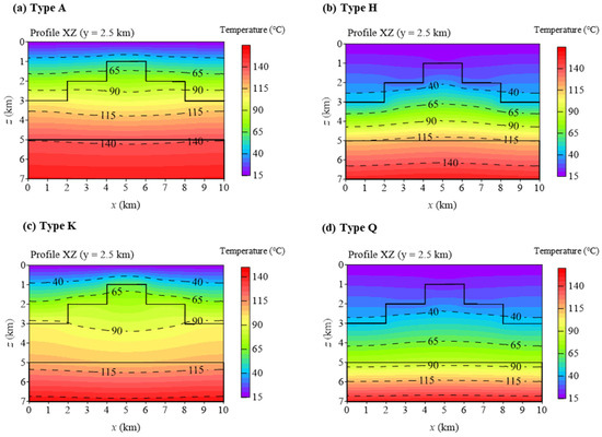
Figure 7.
Vertical cross-section (y = 2.5 km) temperature field through the center of the uplift model.
Across various depth ranges, the temperature field exhibits the following characteristics. Shallow Layer (0–2 km): types A and K exhibit low thermal conductivity, producing steep temperature gradients and elevated temperatures at the top, manifested as convexly arched isotherms. In contrast, types H and Q feature high-conductivity layers that enhance heat dissipation, resulting in flattened temperature profiles and lower top temperatures relative to A and K. Middle Layer (2–4 km): High (or medium) thermal conductivity in types K and Q facilitates rapid thermal energy release, yielding uniform temperature distributions and diminishing gradients. types A and H display intermediate and large temperature gradient variations, respectively, with the latter experiencing abrupt warming in a distinct “thermal barrier” zone. Deep Layer (>4 km): type A’s high basal conductivity inhibits heat accumulation, producing relatively low deep temperatures. types K and H, characterized by moderate conductivity, maintain temperate conditions at depth. type Q’s low-conductivity base promotes heat accumulation, driving anomalous deep-temperature elevation. Thus, Low-conductivity strata induce rapid thermal accumulation in subsequent zones: steep temperature rises occur where thermal resistance is high (e.g., shallow layers of A/K, deep segment of Q, middle layer of H). Conversely, high-conductivity layers act as thermal conduits or dissipators, suppressing abrupt warming (e.g., shallow zones of H/Q, mid-section of K, deep layer of A). The stratigraphic sequence of layer types governs the depth distribution of temperature extremes.
Simultaneously, the temperature “extremum” phenomenon resulting from the combination of high and low thermal conductivity is markedly accentuated in depression types—exemplified by Type Q, where a basal thermal resistance layer of 1.5 W/m·K induces temperatures at 6–7 km depth significantly exceeding those of other types. In uplifted areas, heat dissipation diminishes thermal accumulation effects, narrowing temperature differentials across types. Uplifted regions exhibit upward-warped isothermal surfaces, with central zones displaying lower temperature extremes than peripheral areas; conversely, depression zones feature downward-bending isothermal surfaces, forming “thermal centers”. Temperature variations at varying depths are pronounced in depression-type structures, whereas uplifted areas demonstrate converging differentials with increasing depth.
Collectively, the spatial distribution of the temperature field is “co-controlled” by the thermal conductivity sequence and formation depth—the former governs vertical heat transfer efficiency, while the latter dictates heat flow convergence/divergence pathways: Depression areas coupled with low-conductivity basal layers readily develop deep thermal anomalies, constituting geothermal enrichment zones. Uplifted regions typically exhibit lower temperatures, rendering them suitable for applications such as hydrocarbon reservoir cooling or CO2 sequestration. Specific stratified and zonal evaluations are requisite for different thermal conductivity configurations across varying structural settings.
3.3.3. Thermal Conductivity–Temperature Field Correlation Analysis in an Uplift Model
Figure 8 illustrates the variations in temperature (red curve) and thermal conductivity (blue curve) with depth. Type A exhibits low near-surface conductivity (≤1.5 W/m·K), where the red temperature curve demonstrates the steepest initial slope, indicating a high geothermal gradient (rapid temperature rise). As mid-layer conductivity increases (≥6.0 W/m·K), the temperature slope moderates. The basal high-conductivity layer (>4.0 W/m·K) further reduces the geothermal gradient, yielding the slowest temperature rise. This phenomenon stems from heat accumulation within low-conductivity layers versus efficient heat dissipation in high-conductivity strata, establishing a conductivity-sequence-dependent segmented temperature gradient pattern. Type K features low near-surface conductivity (1.5 W/m·K), abruptly increasing to high mid-layer values (6.0 W/m·K), with moderate basal conductivity (2.7 W/m·K). The temperature curve displays an initially steep ascent in shallow zones, transitioning to a gentler inflection at mid-depths due to the mid-layer’s role as a heat transfer conduit. The basal section exhibits slightly accelerated warming. This configuration promotes thermal equilibration at depth by efficiently dissipating basal heat accumulation through the conductive mid-layer. Type H is characterized by high near-surface conductivity (6.0 W/m·K), sharply dropping to low mid-layer conductivity (1.5 W/m·K), and moderate basal values (2.7 W/m·K). The shallow temperature curve is subdued, reflecting slow heating. The mid-layer low-conductivity zone triggers an abrupt steepening of the red temperature profile, while the basal segment moderates again. Mechanistically, efficient near-surface dissipation maintains cooler shallow zones, whereas the mid-layer traps heat (“thermal locking”), catalyzing rapid temperature escalation. Type Q combines high near-surface conductivity (6.0 W/m·K), moderate mid-layer conductivity (2.7 W/m·K), and low basal conductivity (1.5 W/m·K). It exhibits the shallowest temperature rise gradient, while the basal low-conductivity layer produces an exceptionally steep temperature curve, resulting in the highest deep-temperature amplitude among all types. Dominated by surface heat dissipation and basal thermal barrier formation, this configuration maximizes deep heat accumulation.
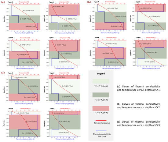
Figure 8.
Thermal conductivity and temperature distribution in the uplift model across different types A, K, H, and Q.
The sectional heating characteristics across all types fundamentally arise from variations in thermal conductivity (λ) and stratigraphic sequencing. Low-λ layers impede heat transfer, accelerating temperature rise (thermal barrier effect), while high-λ layers suppress warming (conduit/dissipation effect), thereby governing zonal geothermal gradient evolution.
The slope of the temperature curve (geothermal gradient, Gt) exhibits a pronounced inverse relationship with segment-specific thermal conductivity, governed by Gt = q/λ. Thus, lower λ accelerates heating (steeper curve), whereas higher λ moderates temperature change (gentler ascent). Key manifestations include:
(1) Layer-boundary inflection points: Temperature curves develop kinks at conductivity interfaces, reflecting abrupt thermal response to physical property transitions.
(2) Segmented regularity: Slope variations in temperature profiles align precisely with step-changes in conductivity curves.
4. Discussion
4.1. Integrated Comparison of the Thermal States of Depression and Uplift Models
The comparative analysis of temperature distributions between uplift and depression structures in AKHQ-type reveals the following distinctive characteristics across varying depths:
In shallow zones, temperatures in uplift models are lower than in depression models. Uplift structures act as “divergent outlets for heat flow,” facilitating lateral and upward heat diffusion, which impedes geothermal accumulation and results in reduced surface temperatures. Conversely, depression structures exhibit pronounced “heat sink” effects, concentrating heat flow in low-lying areas and yielding comparatively higher surface temperatures.
Within deep strata, depression models display universally higher temperatures than uplift models. This phenomenon is particularly amplified in basal layers with low thermal conductivity (e.g., Q-type), where heat dissipation is inhibited, leading to abrupt temperature surges and the formation of “deep thermal islands”. Uplift models, however, experience efficient basal heat dispersion, weakening cumulative thermal effects and constraining peak temperatures in deep zones.
In the Shallow Layer, initial temperature gradients are governed by thermal conductivity contrasts, while topography dictates heat flow pathways—uplift zones promote cooling. In the Deep Layer, Thermal conductivity sequences either amplify or attenuate topographic influences; low-conductivity basal strata in depressions enhance “thermal sealing,” causing anomalous high-temperature anomalies.
As for the Depression Zones, differences among the four types (A, K, H, Q) are accentuated. Q-type depressions exhibit “extreme thermal anomalies,” with bottom temperatures far exceeding other types. A/H-type depressions show thermal accumulation points at the bottom (low conductivity) or middle (moderate conductivity) layers. In the Uplift Zones, Heat flow dispersion suppresses thermal accumulation, causing convergence and homogenization of peak temperatures across models and diminishing inter-type variations.
Overall, the main features are as follows: (1) In uplifted models, the four thermal-conductivity distribution types (A, K, H, Q) govern the piecewise slopes of the temperature curves and the locations of extrema; low-conductivity layers trap heat, whereas high-conductivity layers facilitate heat transfer. (2) The temperature curves exhibit a clear inverse correlation with thermal conductivity, with distinct breakpoints at layer interfaces. (3) By contrast, depression model show higher temperatures at the top, larger extrema at the bottom, and more pronounced inter-type temperature contrasts; their thermal anomalies are stronger than in uplifted model, owing to the coupled effects of topographic focusing/defocusing and basal thermal conductivity. (4) Within any given depth interval, under the A and K types, temperatures in the uplifted model exceed those in the depression model; whereas under the H and Q types, the depression model exhibits higher temperatures than the uplifted model (see Table 2).
Table 2.
Comparison of temperatures at different depths for depression and uplift models of the same type.
In addition, based on the overall analysis and the temperature-field slice characteristics, it is difficult to judge which model is superior by a single criterion; both structural morphology (depression/uplift) and heat-extraction depth must be considered together. Taking the H- and Q-type models as an example: under current technical and economic conditions, the typical medium–deep extraction depth is about 3 km, at which point the H-type is optimal for both depressions and uplifts. When the extraction depth exceeds 5 km, the H-type is relatively preferable in uplift areas, whereas the Q-type is relatively preferable in depression areas. Therefore, model selection should be guided by the coupling of structural type and target depth, rather than a universal comparison of a single model type.
4.2. Analysis of the Thermal Conductivity–Heat Flux Relationship Across Different Formations
As shown in Figure 9, the depression model’s distributions of thermal conductivity and heat flux across different strata are characterized as follows:
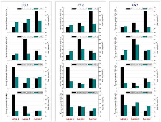
Figure 9.
Heat-flux characteristics versus thermal conductivity in the depression model.
(1) Within each stratigraphic types (A, K, H, Q), from the center (CX1) toward the margin (CX3), the relationship between thermal conductivity and heat flux undergoes a progressive transition from strong positive correlation to weak correlation and, ultimately, to a loose or locally mismatched pattern. Taking the A-type as an example: at CX1, the thermal conductivities of the three strata increase from the first to the third layer, and the heat flux rises synchronously, indicating a clear positive correlation; at CX2, although Layer 2 still preserves this positive correspondence, the amplitude of heat-flux variation among the other layers starts to narrow and the correlation weakens; at the outermost CX3, the heat flux in Layers 1 and 3 becomes lower than that in the middle layer, signaling a local mismatch in interlayer relations. The K- and H-type show a similar behavior: at CX1, layers with higher thermal conductivity carry larger heat fluxes, whereas toward CX2 and CX3 the interlayer flux differences diminish and the correlation progressively decays. In the Q-type, by contrast, at the center (CX1) the high-conductivity layer actually carries a smaller heat flux, implying that topographic concavity/convexity effects render heat-flow partitioning more complex; moving outward, heat flux becomes more evenly distributed across layers and the overall correlation is the weakest. These observations indicate that the conductivity–heat-flux relationship is most robust near the center, whereas toward the edges geometric and boundary-condition effects weaken the positive correlation and may even induce reversed or uncorrelated patterns.
(2) Using the peripheral location CX2 as an example, across the four types (A, K, H, Q), the influence of thermal conductivity on heat flux exhibits a strengthen-then-weaken evolution. In the A-type, the three-layer system maintains a clear positive association between conductivity and heat flux: as conductivity increases from low to high, the flux rises from approximately 48 to 55 mW/m2. In the K-type, the overall conductivity level increases and the baseline heat flux is elevated; however, the interlayer increment in flux narrows slightly relative to A-type, and the strength of association is correspondingly reduced. The H-type further enhances the conductivity of the middle layer, producing a marked surge in its heat flux and bringing the interlayer correlation to a peak. In the Q-type, although interlayer contrasts in conductivity persist, the heat flux tends toward a more uniform distribution; the highest-conductivity layer no longer corresponds to the highest flux, indicating that topographic concavity/convexity reorganizes boundary heat-transfer patterns and attenuates the extent to which conductivity drives heat flow. Overall, from A to H the conductivity–flux coupling first strengthens and reaches a maximum, whereas in the Q-type it weakens again.
Accordingly, in concave terrain, the A/K/H types exhibit a pronounced positive correlation between conductivity and heat flux at the center (CX1), which progressively weakens toward the margins (CX2, CX3) and may even display local mismatches. At a fixed location (e.g., CX2), the correlation strength increases from A to K and peaks at H; upon switching to the concave–convex topography of the Q-type, it declines rapidly, the flux distribution becomes more homogeneous, and high-conductivity layers no longer correspond to high flux. These results indicate that the reshaping of heat-transfer pathways by complex topographic boundary conditions outweighs the influence of conductivity contrasts alone.
As shown in Figure 10, the uplift model’s distributions of thermal conductivity and heat flux across different strata are characterized as follows: (1) Within the same convex topographic setting, from CX1 to CX2 to CX3, the coupling strength between thermal conductivity and heat flux exhibits a “tight-to-loose” progression. In the A-, K-, and H-type, at the central point CX1, layers with higher conductivity carry larger heat fluxes, indicating a pronounced positive correlation; at the intermediate point CX2, the positive correlation persists but interlayer flux contrasts diminish and local mismatches emerge; at the outermost point CX3, high-conductivity layers no longer correspond to high flux, and the correlation structure becomes fragmented or even inverted. By contrast, in the Q-type convex model, the positive correlation is disrupted at all locations: the high-conductivity layer carries the lowest heat flux, the flux distribution becomes more uniform, and the convex geometric effect fundamentally reshapes heat-flow pathways, thereby weakening or reversing the direct driving relationship between conductivity and heat flux.
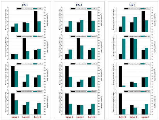
Figure 10.
Distribution of heat flux values across thermal conductivities for the uplift model.
(3) Taking the edge location CX2 as an example, across the A → K → H → Q types the conductivity–heat-flux association alternates in a strong–weak–strong–weak sequence. In the A-type case, the three layers exhibit a consistent positive correlation between thermal conductivity and heat flux. In the K-type case, the layer with the highest conductivity no longer carries the largest flux, and the coupling is markedly weakened. In the H-type case, the most conductive layer regains its advantage and the heat flux again reaches a peak, reinstating the positive correlation. In the Q-type case, the convex boundary conditions substantially reorganize the heat-transfer regime: fluxes across layers converge, the highest-conductivity layer actually carries the least heat flow, and the association nearly vanishes or reverses. This pattern underscores the dominant role of geometry and layering in governing conductivity–flux coupling.
Accordingly, in convex models the positive correlation between thermal conductivity and heat flux is markedly suppressed by geometric boundary reshaping: it is strongest at the center (CX1) and progressively weakens toward the edge (CX3), potentially reversing there. At a fixed location (e.g., CX2), a cross-model comparison from A → K → H → Q exhibits a weak–strong–weak oscillation, with the Q-type showing near-zero or reversed association. These results indicate that the geometric and boundary effects of convex stratigraphic structures dominate the heat-transfer pathways, far outweighing the influence of conductivity contrasts alone.
5. Conclusions
(1) The finite-element three-dimensional heat-transfer algorithm developed in this study attains accuracy exceeding 99% for both depressional and uplifted stratigraphic structure models. We also introduce the A/K/H/Q type, which provides a robust foundation and practical reference for subsequent temperature-field simulations of diverse geothermal geological structures and for three-dimensional inversion of thermal conductivity, among other applications.
(2) In depressional strata, high-temperature reservoirs shallower than 2 km are primarily hosted by A- and K-type formations, whereas mid-to-deep (>3 km) high-temperature zones occur mainly within Q- and H-type structures. In uplifted strata, shallow-to-intermediate (<3 km) high-temperature reservoirs are concentrated in A- and K-type structures; deep high temperatures occur mainly in A- and H-type structures, with A-type exhibiting the higher temperatures.
(3) In the mid-to-deep (>3 km) portions of depressional structures, the temperature fields of A- and H-types exhibit a mirror-image relationship with the stratigraphic architecture, whereas K- and Q-types show the opposite. In the mid-to-deep (>3 km) portions of uplifted structures, A- and K-type temperature fields exhibit a mirror-image relationship with the stratigraphy, whereas H- and K-type show the opposite. At comparable depths, temperatures in uplift models generally exceed those in depression models for A/K-type, while for H/Q-type, temperatures in depressions are generally higher than in uplifts.
(4) The essential differences in temperature distributions arise chiefly from: (i) the absolute values and ordering of layerwise thermal conductivities, which directly control the temperature gradients within individual lithologic intervals; (ii) layer thicknesses and interface depths, which govern the piecewise accumulation of temperature with depth; and (iii) stratigraphic structure (e.g., depression vs. uplift), which redistributes heat-flow density and pathways, producing local “hot islands” or “cold zones”. Overall, lower thermal conductivity yields larger geothermal gradients and a faster temperature increase with depth, whereas higher conductivity facilitates more uniform heat dissipation, thereby mitigating local warming.
(5) Regardless of depression or uplift, A/K/H types exhibit a strong positive correlation between thermal conductivity and heat flux at the center (CX1), which weakens toward the margins (CX2, CX3); the Q-type configuration markedly attenuates this correlation and promotes a more uniform flux distribution. The two settings differ in that: in depressions, the correlation strength increases monotonically from A → K → H and then drops sharply in Q due to geometric focusing of heat flow; in uplifts, the correlation decays from CX1 → CX3 and may even reverse, and at a fixed location the cross-type sequence A → K → H → Q shows a weak–strong–weak fluctuation, reflecting geometric dispersion of heat flow. Hence, the reshaping of heat-transfer pathways by stratigraphic geometry exerts a far greater influence on heat flux than conductivity contrasts alone. Moreover, low-conductivity zones, despite their high geothermal gradients, correspond to low terrestrial heat flow—challenging the conventional assumption that high gradients necessarily coincide with high heat flow. Based on our 3D simulations of temperature and heat flow under varying conductivities, we refine the understanding of regional heat-flow distribution mechanisms. Future geothermal exploration should prioritize “high-gradient–low-heat-flow” coupled zones, using this perspective to optimize target selection and provide a robust theoretical basis for resource assessment.
Author Contributions
Conceptualization, P.C. and G.H.; Methodology, P.C. and G.H.; Software, G.H., J.Y., X.J., J.Z. and N.B.; Validation, L.L., N.W., X.J., J.Z. and N.B.; Formal analysis, L.L., N.W., X.J., N.B. and H.D.; Investigation, P.C., X.J. and N.B.; Resources, P.C. and J.Z.; Data curation, L.L., J.Y., N.W., X.J. and H.D.; Writing—original draft, G.H. and N.W.; Writing—review & editing, G.H., J.Y., N.W., X.J., N.B. and H.D.; Visualization, P.C., L.L., J.Z. and H.D.; Supervision, P.C.; Project administration, P.C.; Funding acquisition, P.C. and G.H. All authors have read and agreed to the published version of the manuscript.
Funding
This research was funded by the Scientific and Technologial Innovation Programs of Higher Education Institutions in Shanxi (No. 2023L388, No. 2021L585), the National Nature Science Foundation of China (No. 42404097, No. U2344218), the Deep Earth Probe and Mineral Resources Exploration-National Science and Technology Major Project (No. 2024ZD1003600), and the Nature Science Foundation of Shanxi Province (No. 202303021212310, No. 202203021211288). We also acknowledge the editors and reviewers for their constructive suggestions and comments.
Data Availability Statement
The data presented in this study are available on request from the corresponding author, due to restrictions that make them not publicly accessible at present.
Conflicts of Interest
Author Pengfei Chi was employed by the Shanxi Second Geological Engineering Exploration Institute Co., Ltd. The remaining authors declare that the research was conducted in the absence of any commercial or financial relationships that could be construed as a potential conflict of interest.
References
- Esen, H.; Inalli, M.; Esen, M. Numerical and experimental analysis of a horizontal ground-coupled heat pump system. Build. Environ. 2007, 42, 1126–1134. [Google Scholar] [CrossRef]
- Balbay, A.; Esen, M. Temperature distributions in pavement and bridge slabs heated by using vertical ground-source heat pump systems. Acta Sci. Technol. 2013, 35, 677–685. [Google Scholar] [CrossRef]
- Gharibi, S.; Mortezazadeh, E.; Bodi, S.J.H.A.; Vatani, A. Feasibility study of geothermal heat extraction from abandoned oil wells using a U-tube heat exchanger. Energy 2018, 153, 554–567. [Google Scholar] [CrossRef]
- Nian, Y.-L.; Cheng, W.-L. Evaluation of geothermal heating from abandoned oil wells. Energy 2018, 142, 592–607. [Google Scholar] [CrossRef]
- Sayigh, A. Renewable energy—The way forward. Appl. Energy 1999, 64, 15–30. [Google Scholar] [CrossRef]
- Gupta, H.K.; Roy, S. Geothermal Energy: An Alternative Resource for the 21st Century; Elsevier: Amsterdam, The Netherlands, 2006. [Google Scholar]
- Adams, B.M.; Kuehn, T.H.; Bielicki, J.M.; Randolph, J.B.; Saar, M.O. On the importance of the thermosiphon effect in CPG (CO2 plume geothermal) power systems. Energy 2014, 69, 409–418. [Google Scholar] [CrossRef]
- Aliyu, M.D.; Chen, H.-P. Sensitivity analysis of deep geothermal reservoir: Effect of reservoir parameters on production temperature. Energy 2017, 129, 101–113. [Google Scholar] [CrossRef]
- Arat, H.; Arslan, O. Exergoeconomic analysis of district heating system boosted by the geothermal heat pump. Energy 2017, 119, 1159–1170. [Google Scholar] [CrossRef]
- Liu, Y.; Hou, J.; Zhao, H.; Liu, X.; Xia, Z. A method to recover natural gas hydrates with geothermal energy conveyed by CO2. Energy 2018, 144, 265–278. [Google Scholar] [CrossRef]
- Tester, J.W.; Anderson, B.J.; Batchelor, A.; Blackwell, D.; DiPippo, R.; Drake, E.; Garnish, J.; Livesay, B.; Moore, M.; Nichols, K.; et al. The future of geothermal energy. Mass. Inst. Technol. 2006, 358, 1–3. [Google Scholar]
- Wu, J.; Huang, X.; Huang, G.; Peng, R.; Zhou, W. Status and prospects of electromagnetic method used in geothermal resources exploration. Acta Geosci. Sin. 2023, 44, 191–199. [Google Scholar]
- Li, Q.; Wu, J.; Li, Q.; Wang, F.; Cheng, Y. Sediment instability caused by gas production from hydrate-bearing sediment in Northern South China Sea by horizontal wellbore: Sensitivity analysis. Nat. Resour. Res. 2025, 34, 1667–1699. [Google Scholar] [CrossRef]
- Li, Q. Reservoir Science: A multi-coupling communication platform to promote energy transformation, climate change and environmental protection. Reserv. Sci. 2025, 1, 1–2. [Google Scholar] [CrossRef]
- Lee, K.S. Effects of regional groundwater flow on the performance of an aquifer thermal energy storage system under continuous operation. Hydrogeol. J. 2014, 22, 251–262. [Google Scholar] [CrossRef]
- Chapman, D.S.; Rybach, L. Heat flow anomalies and their interpretation. J. Geodyn. 1985, 4, 3–37. [Google Scholar] [CrossRef]
- Zhou, J.; Hu, X.; Cai, H. Three-dimensional finite-element analysis of magnetotelluric data using Coulomb-gauged potentials in general anisotropic media. Pure Appl. Geophys. 2021, 178, 4561–4581. [Google Scholar] [CrossRef]
- Rybach, L.; Bodmer, P.; Pavoni, N.; Mueller, S. Siting criteria for heat extraction from hot dry rock; Application to Switzerland. Pure Appl. Geophys. 1978, 116, 1211–1224. [Google Scholar] [CrossRef]
- Mao, X. Genetic mechanism and distribution characteristics of high temperature anomaly in geothermal field. Acta Geosci. Sin. 2018, 39, 216–224. [Google Scholar]
- Berktold, A. Electromagnetic studies in geothermal regions. Geophys. Surv. 1983, 6, 173–200. [Google Scholar] [CrossRef]
- Urzua, L.; Powell, T.; Cumming, W.B.; Dobson, P. Apacheta, a New Geothermal Prospect in Northern Chile. 2002. Available online: https://www.osti.gov/biblio/815476 (accessed on 11 September 2025).
- Oskooi, B.; Pedersen, L.B.; Smirnov, M.; Árnason, K.; Eysteinsson, H.; Manzella, A.; Group, D.W. The deep geothermal structure of the Mid-Atlantic Ridge deduced from MT data in SW Iceland. Phys. Earth Planet. Inter. 2005, 150, 183–195. [Google Scholar] [CrossRef]
- Wang, L.S.; Liu, S.W.; Xiao, W.Y.; Li, C.; Li, H.; Guo, S.P.; Liu, B.; Luo, Y.H.; Cai, D.S. Distribution characteristics of terrestrial heat flow in Bohai Bay Basin. Chin. Sci. Bull. 2002, 47, 151–155. [Google Scholar]
- Roy, R.F.; Blackwell, D.D.; Decker, E.R. Continental heat flow. In The Nature of the Solid Earth; McGraw-Hill: Columbus, OH, USA, 1972; pp. 506–543. [Google Scholar]
- Villas, R.; Norton, D. Irreversible mass transfer between circulating hydrothermal fluids and the Mayflower stock. Econ. Geol. 1977, 72, 1471–1504. [Google Scholar] [CrossRef]
- Medina Martínez, F. Applications of continuum physics to geological problems/DL Turcotte y G. Schubert. Geofis. Int. 1986, 25, 475–476. [Google Scholar] [CrossRef]
- McBirney, A.R. Igneous Petrology; Jones & Bartlett Learning: Burlington, MA, USA, 1993. [Google Scholar]
- Gao, Z.J.; Wu, L.J.; Cao, H. The Summarization of Geothermal Resources and Its Exploitation and Utilization in Shandong Province. J. Shandong Univ. Sci. Technol.-Nat. Sci. 2009, 28, 1–7. [Google Scholar]
- Mao, X.P.; Chen, X.R. Discussion on Heat Flow Distribution Characteristics and Terrestrial Heat Flow. Coal Geol. China 2025, 37, 1–9. [Google Scholar]
- Huang, G.; Hu, X.; Cai, J.; Ma, H.; Chen, B.; Liao, C.; Zhang, S.; Zhou, W. Subsurface temperature prediction by means of the coefficient correction method of the optimal temperature: A case study in the Xiong’an New Area, China. Geophysics 2022, 87, B269–B285. [Google Scholar] [CrossRef]
- Huang, G.; Hu, X.; Liu, S.; Peng, R.; Zhou, J.; Bai, N.; Liu, L.; Mu, M. Deep temperature-field prediction utilizing the temperature–pressure-coupled resistivity model: A case study in the Xiong’an new area, China. IEEE Trans. Geosci. Remote Sens. 2023, 62, 1–16. [Google Scholar] [CrossRef]
- Fang, L. Heat Transfer Analysis and Application of Deep Borehole Heat Exchanger in Ground Source Heat Pump System. Ph.D. Thesis, Shandong Jianzhu University, Jinan, China, 2018. [Google Scholar]
- Zhang, W.; Wang, J.; Zhang, F.; Lu, W.; Cui, P.; Guan, C.; Yu, M.; Fang, Z. Heat transfer analysis of U-type deep borehole heat exchangers of geothermal energy. Energy Build. 2021, 237, 110794. [Google Scholar] [CrossRef]
- Huang, G.; Hu, X.; Ma, H.; Liu, L.; Yang, J.; Zhou, W.; Liao, W.; Bai, N. Optimized geothermal energy extraction from hot dry rocks using a horizontal well with different exploitation schemes. Geotherm. Energy 2023, 11, 5. [Google Scholar] [CrossRef]
- Xu, S.Z. The Finite Element in Geophysics; Science Press: Beijing, China, 1994. [Google Scholar]
- Freymark, J.; Sippel, J.; Scheck-Wenderoth, M.; Bär, K.; Stiller, M.; Fritsche, J.-G.; Kracht, M. The deep thermal field of the Upper Rhine Graben. Tectonophysics 2017, 694, 114–129. [Google Scholar] [CrossRef]
- Cai, H.; Xiong, B.; Han, M.; Zhdanov, M. 3D controlled-source electromagnetic modeling in anisotropic medium using edge-based finite element method. Comput. Geosci. 2014, 73, 164–176. [Google Scholar] [CrossRef]
- Bai, N.; Zhou, J.; Hu, X.; Han, B. 3D edge-based and nodal finite element modeling of magnetotelluric in general anisotropic media. Comput. Geosci. 2022, 158, 104975. [Google Scholar] [CrossRef]
- Yang, J.; Huang, G.; Hu, X. A 3D thermal conductivity prediction method for deep strata based on temperature field estimation. Geophysics 2023, 88, B297–B316. [Google Scholar] [CrossRef]


Disclaimer/Publisher’s Note: The statements, opinions and data contained in all publications are solely those of the individual author(s) and contributor(s) and not of MDPI and/or the editor(s). MDPI and/or the editor(s) disclaim responsibility for any injury to people or property resulting from any ideas, methods, instructions or products referred to in the content. |
© 2025 by the authors. Licensee MDPI, Basel, Switzerland. This article is an open access article distributed under the terms and conditions of the Creative Commons Attribution (CC BY) license (https://creativecommons.org/licenses/by/4.0/).