Abstract
This paper presents a data-driven decision-support framework for distribution system operations using logistic regression (LR) on the Voltage Margin Index (VMI). Treating VMI as the sole explanatory feature, the proposed two-stage workflow first fits an inferential LR model to establish statistical significance and perform valid statistical inference on the coefficients. Next, it trains a performance-optimized LR classifier with class-balanced sample weighting to produce calibrated violation probabilities. LR maps VMI to violation probability and analytically converts a calibrated probability threshold into an operator-ready VMI decision boundary. Applying 5-fold group cross-validation to 8816 node-level samples generated from a 22.9 kV Jeju Island model yields performance- and safety-oriented probability thresholds (θopt = 0.7891, θsafe = 0.6880), which correspond to VMI decision boundaries VMIDB,opt = 0.7893 and VMIDB,safe = 0.8101. On an unseen 20% test set, the LR classifier achieves 99.94% accuracy (F1 = 0.9977) under θopt and 100% recall under θsafe. A random forest (RF) benchmark confirms comparable accuracy (=99.72%) but lacks analytical invertibility and transparency. This framework offers distribution system operators (DSOs) and virtual power plant (VPP) operators clear, evidence-based criteria for routine planning and risk-averse decision-making, and it can be applied directly to any distribution system with node-level voltage measurements and known regulation limits.
1. Introduction
In line with the global energy transition, distributed energy resources (DERs) based on renewable energy, such as photovoltaic (PV) and wind turbine (WT) systems, are being rapidly integrated into distribution systems. Unlike traditional distribution systems with unidirectional power flows, an increase in DERs introduces bidirectional power flows, significantly increasing the complexity and uncertainty of the system. This change poses new challenges, particularly in terms of voltage management. On sunny days, generation from DERs can exceed local load demand, causing reverse power flows that may lead to overvoltage problems exceeding regulatory limits. Conversely, at other times, localized voltage drops can result in undervoltage issues [1]. Distribution system operators (DSOs) must effectively manage voltage problems to maintain grid stability and reliability. Therefore, a reliable tool is essential to assess in advance which nodes are more vulnerable to voltage violations and to quantify the potential risks. This provides an objective basis for critical decision-making processes, such as approving new DER interconnections or prioritizing grid reinforcement plans. To this end, establishing a clear criterion that DSOs can intuitively understand and apply in the field, namely, a decision boundary distinguishing ‘safe’ from ‘at-risk’ states, has become urgent.
Initial studies for establishing such a decision boundary mainly focused on utilizing traditional voltage stability indices (VSIs) such as the L-index [2] or evaluating system stability through analytical methods based on power flow calculations [3]. However, these classical approaches are biased toward static stability limit analysis under fixed operating points and have suffered from a high computational burden and heavy reliance on the accuracy of the system model when analyzing multiple scenarios. To overcome these limitations, data-driven studies that directly learn the statistical characteristics of systems from actual measurement data or large-scale simulation data are being actively pursued. An early machine learning (ML) approach was used to determine the hosting capacity of DERs using a decision tree [4], but this method yielded a complex set of if–then rules and did not provide a single intuitive decision boundary for DSOs. More recently, studies have emerged that generate operating rules directly from data, but the resulting rules are often complex, multivariable expressions and lack intuitiveness [5]. To achieve higher prediction accuracy, research utilizing complex nonlinear models such as artificial neural networks (ANNs) and support vector machines (SVMs) has become mainstream, and this trend is similarly observed in the hosting capacity assessment of low-voltage systems [6,7,8,9]. Furthermore, model complexity continues to increase, for instance, by learning spatio-temporal features [10] or by introducing advanced deep learning techniques like Generative Adversarial Networks (GANs) [11]. However, these black-box models hinder explanation of causal relationships for individual predictions and cannot readily yield analytical decision boundaries for voltage violations.
Researchers have also approached the problem from different perspectives. Some studies, for instance, have framed it as an optimization task, maximizing hosting capacity [12] or selecting optimal DER sites [13], or focused on determining the feasible operating region for stable system operation [14]. Furthermore, online control for real-time violation management [15] and correction control models to rectify predicted instability [16] are prominent research areas, while sensitivity analysis quantifies the voltage impact of specific variables [17]. However, because these methods serve distinct purposes, including long-term planning and real-time control, they have yet to yield a clear, pre-emptive decision boundary for assessing node-specific risks or guiding long-term operational policies. Recently, several studies have addressed the practical constraints of incomplete data. Prediction in unobservable systems, where measurements are missing, requires state estimation, a separate, complex research field [18,19]. Moreover, privacy-preserving decentralized prediction frameworks increase system complexity [20]. Attempts to capture voltage-state ambiguity using fuzzy logic [21] have likewise complicated the establishment of clear pass/fail criteria for DSOs. Beyond these approaches, voltage violation risk inherently involves uncertainty, making probabilistic risk assessment essential [22,23]. In this context, logistic regression (LR) draws attention for offering both probabilistic outputs and model interpretability [24]. However, most existing studies have yet to directly link a single physically meaningful index, such as the Voltage Margin Index (VMI), to violation probability and then analytically invert that relationship to derive actionable decision boundaries.
Therefore, this paper proposes a new framework for assessing voltage violation risk to overcome the aforementioned limitations. It uses the VMI, which intuitively represents the voltage margin of the distribution system, as a single explanatory variable and establishes an explicit relationship between VMI and the probability of voltage violation through a statistically validated LR model. Finally, this relationship is analytically inverted to derive performance-oriented and safety-oriented VMI decision boundaries, providing DSOs and virtual power plant (VPP) operators with clear, data-driven criteria for critical operational decisions. The main contributions of this paper are as follows:
- An Interpretable Yet High-Performance Model: We introduce an interpretable model that combines the physically meaningful VMI with a simple LR, avoiding black-box complexity. VMI is leveraged as a powerful single predictor, justified by its ability to synthesize system-wide effects and its validated statistical significance (p < 0.001). Benchmarking against a random forest (RF) classifier confirms that this transparent approach achieves high reliability without sacrificing predictive power.
- Derivation of Analytical and Generalizable Decision Boundaries: We leverage the LR model’s closed-form nature to analytically derive absolute VMI decision boundaries from its probability thresholds. This methodology, validated via 5-fold cross-validation on detailed simulation data from Jeju Island, yields specific, actionable criteria: a performance-oriented boundary of 0.7893 and a safety-oriented boundary of 0.8101. Crucially, the LR derivation procedure can be applied unchanged to any system with node-level voltage measurements and known regulation limits.
- Enhanced Decision Support for Grid Operations: The resulting VMI boundaries provide DSOs and VPP operators with clear, data-driven criteria for critical tasks. The performance-oriented boundary is suited for routine operational planning, while the safety-oriented boundary provides a robust, risk-averse criterion for high-stakes decisions like DER interconnection approval and grid reinforcement. This framework replaces operational ambiguity with transparent, statistically grounded criteria, enhancing decision-making objectivity.
The remainder of this paper is organized as follows. Section 2 explains the theoretical background of VMI and LR. Section 3 describes the data generation and the proposed methodology in detail, and Section 4 introduces the simulation environment that models a real distribution system. In Section 5, the simulation results are analyzed, and the superiority of the proposed technique is verified through comparison with a benchmark model. Finally, Section 6 concludes this paper and presents future work.
2. Related Research and Theoretical Background
2.1. Voltage Margin Index (VMI)
The VMI is a dimensionless, node-level metric that quantifies the long-term margin between the actual line-to-line voltage at each node and the statutory voltage regulation range of the distribution system. By condensing instantaneous measurements into a single scalar value, the VMI accounts for both overvoltage and under-voltage tendencies. This makes it an intuitive indicator of per-node voltage robustness. Moreover, the VMI was proposed as an index to evaluate which nodes or feeders are most suitable for DER interconnection by comparing their relative voltage stability profiles [25]. The VMI formulation starts with an instantaneous voltage margin. For node i at sampling instant t, the measured voltage is Vi,t, the nominal voltage is Vnom, and the upper and lower limits of the statutory voltage regulation range are Vmax and Vmin, respectively. Because these limits are incorporated directly as parameters, this formulation remains valid for any symmetric or asymmetric regulation range (e.g., ±5% or +5/−8% around Vnom) without further adjustment.
The instantaneous voltage margin (VMi,t) is defined piecewise to account for overvoltage and undervoltage conditions as follows:
Both expressions normalize the margin by the corresponding segment of the voltage regulation range. They include a squared penalty term that reduces the margin to zero as the voltage approaches the pertinent bound of that range. If the fraction inside the squared term exceeds unity, the result becomes negative, signaling a violation and quantifying its severity by the square of the exceedance. To form a long-term indicator, these instantaneous margins are averaged over the analysis horizon T, producing the node-level VMIi as:
By construction, a VMIi value close to unity indicates that node i operates safely inside the voltage regulation range for most of the study period, implying a low probability of voltage violations. Conversely, a value approaching zero reveals persistent proximity to the regulatory limits and, hence, a high risk of overvoltage or undervoltage events that may necessitate corrective action.
2.2. Limitations of VMI
Despite its effectiveness in ranking nodes or feeders by relative voltage stability, the VMI exhibits two practical limitations. The first arises from the fact that VMI is a time average of instantaneous margins, which smooths out extreme events; a node that experiences brief but severe over- or under-voltage can still report a deceptively benign VMI if the remaining samples are well-behaved. Moreover, VMI functions as a comparative index without a rigorously justified decision boundary to distinguish “safe” from “unsafe” operation, leaving DSOs without an absolute criterion for DER interconnection approval or grid reinforcement decisions.
To overcome these barriers, this paper develops an LR framework that treats the VMI as the sole explanatory variable, converts it into a probabilistic estimate of voltage violation risk, and extracts statistically validated absolute VMI decision boundaries in closed form. Prior work has used VMI primarily for relative comparisons of node or feeder conditions [25]; in contrast, the present framework establishes a probabilistic link from VMI to violation risk via logistic regression, calibrates performance- and safety-oriented thresholds using grouped cross-validation, and translates those thresholds analytically into operator-ready VMI boundaries. Rather than relying solely on a time-averaged VMI, the approach first derives time-step violation indicators and then aggregates them into a node-level label over the analysis horizon. For learning, each sample is built from a node under an operating condition and its time series, using the horizon-averaged VMI as a single scalar feature and the aggregated binary label as the target. As a result, DSOs gain transparent, evidence-based guidance for both relative ranking and absolute acceptance decisions. This framework enables accurate identification of vulnerable network sections, prioritization of reinforcement or maintenance tasks, and continuous monitoring of grid security under diverse operating conditions.
2.3. Logistic Regression Overview
While the VMI offers an intuitive metric for node-level voltage stability, a systematic framework is required to translate this index into a probabilistic assessment of voltage violations. To this end, this paper employs LR, a classical statistical method that has become a cornerstone of supervised ML for binary classification tasks [26,27]. The objective is to find a mapping from an input feature x to a categorical label y ∈ {0, 1}. In the context of voltage stability monitoring, the label y represents the presence (y = 1) or absence (y = 0) of a voltage violation. This paper confines the input to a single explanatory feature (x = VMI) for two primary reasons. First, as an index computed directly from voltage time series data, the VMI inherently synthesizes the aggregate effects of numerous underlying system variables (e.g., load levels, DER generation, and network conditions). Second, this single-variable approach maximizes model interpretability, enabling a clear analysis of the relationship between voltage margin and violation risk.
The model is trained on a data set , which is formally denoted as:
Here, each pair (xk, yk) constitutes a single observation, where xk is the VMI value for the kth sample, and yk is its corresponding binary violation label. The total number of samples in the training set is represented by K. The goal of the learning algorithm is to use this data set to approximate the conditional probability (y = 1|x), which quantifies the likelihood of a voltage violation given a specific VMI value. LR offers the most parsimonious probabilistic classifier while retaining full statistical interpretability. Its hypothesis function is based on the sigmoid function, σ(·), and is written as:
The left-hand side, (y = 1|x), denotes the predicted probability of a voltage violation (y = 1) given an input VMI value (x). The sigmoid function maps the linear combination ωx + b (also known as the logit) into a value between 0 and 1, suitable for a probability estimate. The parameters ω (slope) and b (intercept) are estimated from the data, typically via maximum likelihood estimation. These parameters have direct engineering meaning; a negative coefficient (ω < 0) indicates that as the VMI increases, the predicted probability of a violation decreases, aligning with the intuitive notion that a larger voltage margin implies safer operation. This transparent, closed-form relationship makes LR a powerful foundation for the methodology described in Section 3, where it is used to derive analytical VMI decision boundaries.
3. Research Methodology
3.1. Data Acquisition and Pre-Processing
To operationalize the LR model described in Section 2, a systematic data processing pipeline is required to construct a suitable data set from raw measurements. The proposed workflow consists of three main steps.
3.1.1. Data Collection and VMI Computation
Line-to-line voltages (Vi,t) are gathered for every node i over an analysis horizon T, along with the statutory voltage regulation range defined by limits Vmin, Vnom, and Vmax. Each raw voltage sample is then mapped to an instantaneous margin using Equations (1) and (2), and the final node-level VMI is obtained by time-averaging these margins as shown in Equation (3). This entire feature computation process involves simple, non-iterative algebraic operations, ensuring high computational efficiency and linear scalability even with large data sets.
3.1.2. Voltage Violation Labeling
The labeling process begins by generating a binary violation indicator for each node i at each time step t. A value of 1 signifies that the voltage has moved outside the voltage regulation range [Vmin, Vmax], as defined by:
These instantaneous indicators are then aggregated over the horizon T into a single, node-level label yi, which is set to 1 if at least one time step violates the voltage regulation range during T:
In the learning data set, each sample corresponds to one node under a specific operating condition. The feature is the VMI averaged over T. The target is the binary node-level label yi. Because samples are defined at the node level and voltage violations are rare in stable distribution systems, the data set exhibits a significant class imbalance (few yi = 1 vs. many yi = 0). The challenge posed by this imbalance is addressed via sample weighting during model fitting, as detailed in Section 3.2. In summary, the LR model takes the scalar VMI as input and returns a calibrated probability (yi =1|VMI) ∈ [0, 1] that the node violates the voltage regulation range. An operational decision is obtained by applying a calibrated threshold to this probability. The result is a binary outcome with two classes: violation and non-violation.
3.1.3. Data Set Assembly and Validation
After steps 1–2, the pre-processed samples constitute the supervised learning data set defined in Equation (4). Basic integrity checks, for missing values, voltage regulation range consistency, and duplicate entries, are performed, after which the data are grouped by node ID to prevent data leakage across nodes during model training and validation. This modular pre-processing stage delivers a clean and portable data set that accurately reflects the original distribution and is suitable for ML applications.
3.2. Logistic Regression Modeling
With the curated data set from the pre-processing stage, the data are first partitioned for robust model training and validation, followed by the development of the LR model.
3.2.1. Training and Validation Split
To eliminate node-level data leakage, samples were grouped by node ID and then split into 80% for training and validation and 20% for testing using the GroupShuffleSplit function with random_state = 42 [28]. This ensures that no single node’s observations—across all seasons and scenarios—appear in multiple partitions while preserving the class distribution. This 80/20 split is used for both the statsmodels and scikit-learn stages, and the 20% test set remains untouched until final evaluation. Within the 80% training and validation partition, 5-fold cross-validation is implemented for the scikit-learn classifier using the GroupKFold function with n_splits = 5 grouped by node ID [29]. In each fold, one held-out fold serves as a validation set for probability threshold tuning, and the remaining folds are used for model training. The final performance is evaluated on the untouched 20% test set.
3.2.2. Model Training and Statistical Inference
To combine statistical interpretability with robust prediction, this paper adopts a dual-library approach for LR modeling. This methodology involves two distinct stages: first, establishing the theoretical validity of the explanatory variable using statsmodels, and second, building a performance-optimized predictive tool using scikit-learn [30,31].
The statistical validity of the VMI is first assessed by fitting a single-feature LR model in statsmodels with ℓ2 regularization, a common technique to prevent model overfitting by penalizing large coefficient values. The statsmodels model is fitted on the 80% training and validation data. This process enables the computation of approximate standard errors and p-values, which confirm that the relationship between VMI and voltage violations is statistically significant and robust. A performance-optimized classifier is subsequently built using the LogisticRegression function from scikit-learn. To address the class imbalance in the data set, the class_weight parameter was set to ‘balanced’, which assigns higher weight to the rare violation samples. The classifier uses an ℓ2 penalty with C = 1.0, selected by grouped 5-fold cross-validation within the 80% training and validation partition to balance underfitting and overfitting. This combination stabilizes estimation, mitigates (quasi-)separation, and improves robustness and calibration in rare-event logistic models [32,33]. The ‘liblinear’ solver is employed for efficient convergence, and random_state = 42 is fixed to ensure deterministic behavior and reproducibility [28,34]. This second stage yields the calibrated probability estimates essential for the subsequent threshold-selection procedure.
The final VMI decision boundaries are derived from this performance-optimized model. A key property of the LR model is its analytical tractability; its closed-form logit function allows the fitted coefficients to be analytically inverted to derive absolute VMI decision boundaries. This provides full transparency in deriving operational criteria. Although the coefficients from the inferential and performance-optimized models differ due to their distinct objectives, this two-step approach ensures that our final decision boundaries combine high predictive performance with rigorous statistical validation.
3.3. Threshold Determination Procedure
The LR model provides, for each validation sample, a calibrated probability (y = 1|x) of a voltage violation. Given class imbalance, precision–recall (PR) curves and average precision (AP) are more informative than receiver operating characteristic (ROC) curves; accordingly, PR/AP are reported alongside F1 [35]. First, two parallel procedures convert the calibrated probabilities into a performance-oriented probability threshold (θopt) and a safety-oriented probability threshold (θsafe). Next, these thresholds are analytically inverted to yield absolute VMI decision boundaries. Finally, the applicability of the derived decision boundaries for real-world deployment is discussed.
3.3.1. Performance-Oriented Probability Threshold
θopt is determined based on the F1-score, which is defined as the harmonic mean of precision and recall at a given probability threshold θ [36]:
Here, Precision(θ) is the fraction of true-violation samples among all samples predicted as positive (y = 1|x) ≥ θ, while Recall(θ) is the fraction of actual violations correctly identified. This F1-score maximization is performed within each of the five validation folds described previously. The final θopt is then defined as the arithmetic mean of the fold-wise optima from the five validation folds, {θopt,1, …, θopt,5}.
3.3.2. Safety-Oriented Probability Threshold
In power system operations, failing to detect a potential voltage violation can pose critical risks, including equipment damage, protection system malfunction, and, in severe cases, localized outages. Given these critical risks, a decision criterion that ensures no potential violation goes undetected is essential for secure grid operation. To this end, θsafe is chosen to ensure that no observed violation in the validation set is missed. Within each fold, the minimum nonzero value of (y = 1|x) among all true-violation samples is taken as that fold’s θsafe. The global θsafe is the minimum of these fold-wise thresholds. By construction, applying θsafe ensures zero false negatives in the validation set, at the expense of increased false positives.
3.3.3. Analytical Inversion to VMI
The decision function of the LR model relates θ to VMI via the logit transform:
where b gives the baseline log-odds when VMI = 0, and ω gives the change in log-odds per unit increase in VMI. For instance, a 0.01 increase in VMI changes the log-odds by 0.01ω. Inverting Equation (9) yields the absolute VMI decision boundary corresponding to θ:
Substituting θopt produces the performance-oriented VMI decision boundary (VMIDB,opt), while substituting θsafe produces the safety-oriented VMI decision boundary (VMIDB,safe). Because the ℓ2-penalized estimate yields ω < 0, the logit slope remains negative: lower θ corresponds to higher (safer) VMI decision boundaries, consistent with the interpretation that increasing VMI strongly reduces violation risk. The overall workflow is summarized in the flowchart of Figure 1.
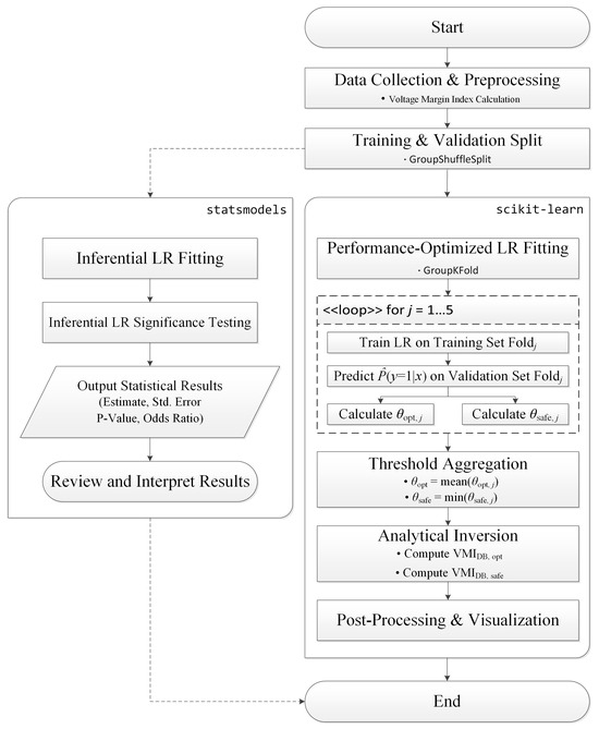
Figure 1.
Flowchart of VMI decision boundary determination.
3.3.4. Applicability
This procedure, which combines threshold selection via validation and analytical inversion, relies solely on the coefficients of the LR model and the probabilities used in validation. It can be applied without modification to any distribution system with node-level voltage measurements and a known voltage regulation range. Adjustments to θopt or θsafe allow tailoring to local risk tolerances, and exact VMI decision boundaries can be derived using Equation (10).
3.4. Benchmark Model: Random Forest
To verify that the LR interpretability does not sacrifice predictive power, the RF classifier was trained on the same data set as a nonlinear benchmark. The classifier was configured with an ensemble of 100 trees using n_estimators = 100, the Gini impurity criterion via criterion = ‘gini’, and unrestricted maximum tree depth using max_depth = None [37]. For a fair comparison, the class_weight parameter was set to ‘balanced’, and random_state was fixed to 42. The same machine learning pipeline detailed in Section 3.2—including data partitioning, cross-validation, and threshold determination—was then applied to the RF model.
However, a critical distinction is that the RF model lacks a closed-form analytical inverse. Therefore, its thresholds cannot undergo analytical inversion to VMI decision boundaries. Instead, approximate VMI decision boundaries were estimated by locating the VMI value on the RF model’s predicted probability curve corresponding to each threshold. Thus, the RF model serves purely as a performance benchmark, confirming that the LR model achieves comparable predictive accuracy; all final, actionable VMI decision boundaries come from the LR model.
4. Case Study and Data Generation
4.1. Jeju Distribution System Model
To assess the generality of the proposed framework, a simplified 22.9 kV model of Jeju Island’s distribution system was developed based on operating data from the Korea Electric Power Corporation (KEPCO). The model partitions the island into six service areas, denoted A through F, as shown in the single-line diagram in Figure 2. Each area is supplied by a single 154/22.9 kV 60 MVA substation, and all distribution lines are standardized using ACSR-160 mm2 conductors [38]. An aggregate load of 13 MW (0.95 power factor) is distributed across feeders in proportion to their node counts.
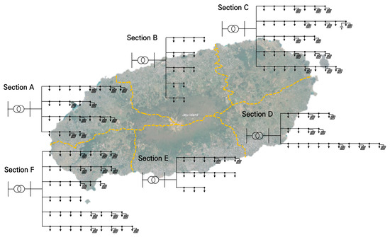
Figure 2.
Single-line diagram of the distribution system model.
The rated capacities and types of DERs vary significantly across the areas, as summarized in Table 1. Areas A and F host 48 MW and 31.5 MW of PV capacity, respectively; Area C integrates 34.8 MW of PV and 2 MW of WT; and Areas D and E connect small-scale PV plants of 8.6 MW and 3.9 MW. Notably, Area B contains no DERs, and both Areas B and E are identified as urban zones. This complete system model was implemented in OpenDSS v9.7.1.1 [39].

Table 1.
Feeder and DER configuration by area.
4.2. Simulation and Data Set Creation
To generate the data set for the ML models, time-series simulations were performed using the OpenDSS model. The simulations were designed to capture a wide range of operating conditions by incorporating distinct seasonal patterns for both load and renewable generation. These patterns were derived from 2021 real-world data, with hourly load profiles from Jeju Island [40] and corresponding generation profiles for PV and WT systems from the Korea Power Exchange [41]. The data reflect typical seasonal variations, such as higher cooling demand on summer evenings and peak PV production on spring afternoons.
For each of the four seasons, these load and generation profiles were applied to the system model to calculate the hourly voltage time series for every node over a 24 h period. In all simulations, the statutory voltage regulation range was set from 20.8 to 23.8 kV, corresponding to an asymmetric deviation of −9.08%/+3.93% from the nominal 22.9 kV permitted by South Korean regulations [42]. Any voltage outside this range was labeled as a violation in the time series. Following the exact procedure detailed in Section 3.1, the resulting raw voltage data were then converted into the final (VMI, label) samples. Specifically, for each operating condition (e.g., season/scenario) and each node, the feature is the VMI obtained by averaging the instantaneous margins over the 24 h horizon, and the label is defined at the node level according to Equation (7): it is set to 1 if any time step within that horizon violates the voltage regulation range and 0 otherwise. This process yielded 8816 samples spanning all nodes and operating conditions.
5. Results and Discussion
5.1. Data Set Composition and Partitioning
The data set of 8816 samples, each comprising a VMI value and a binary violation label, was split into an 80% training and validation set (7054 samples) and a 20% test set (1762 samples), as detailed in Table 2. The training-validation set comprised 6168 non-violation samples (87.4%) and 886 violation samples (12.6%). The test set comprised 1542 non-violation samples (87.5%) and 220 violation samples (12.5%). The consistent class ratio (~12.6% positive, ~87.4% negative) across both partitions ensures a balanced and representative performance evaluation.
Table 2.
Data set composition and class balance.
5.2. Statistical Validation and Interpretation
To build a reliable predictive model, it is essential to first validate the statistical significance of its core explanatory variable. Therefore, before assessing predictive performance, the relationship between VMI and voltage violations was analyzed using an ℓ2-penalized LR model. Table 3 reports penalized-likelihood-based approximate statistical estimates (coefficients, standard errors, p-values, and odds ratios), indicating that VMI is a strong predictor of voltage violations. Because estimation is performed under ℓ2-penalized likelihood, the associated standard errors and p-values are computed from penalized information and should be interpreted as approximate [33,43].
Table 3.
LR coefficients and odds ratios.
The analysis yields a large negative coefficient for VMI (ω = −59.0387 ± 0.7662), indicating that as VMI increases, the log-odds of a violation decrease markedly. This relationship is confirmed to be statistically significant (p < 0.001) and is further quantified by an odds ratio of 2.29 × 10⁻²⁶, implying that a one-unit increase in VMI reduces the odds of a violation to virtually zero. The model’s intercept (b = 46.4803) is also highly significant (p < 0.001) and represents the theoretical log-odds of a violation when VMI is zero. In summary, the statistical analysis demonstrates that VMI is more than a convenient metric; it is a statistically robust and powerful predictor of voltage violations. These results establish a firm foundation for the performance-oriented predictive model presented in the next section.
5.3. Model Performance and Decision Boundary Derivation
Following statistical validation of VMI, a performance-optimized LR classifier was developed. This section describes the derivation of its decision boundaries and evaluates predictive performance on the held-out test set.
5.3.1. Cross-Validated Threshold Selection
Operational criteria were established by first deriving two distinct thresholds from the training and validation sets via a 5-fold group cross-validation strategy. θopt was defined as the average of the fold-wise thresholds that maximized the F1-score, balancing precision and recall. θsafe was set to the minimum threshold across all folds that guaranteed zero false negatives (i.e., perfect recall), prioritizing risk aversion. These thresholds were then analytically inverted using Equation (10) to calculate their corresponding VMI decision boundaries. The final, aggregated values are summarized in Table 4. The threshold selection process is visualized in Figure 3 and Figure 4. The PR curve in Figure 3 shows excellent discrimination (AP = 0.9908).
Table 4.
LR cross-validation thresholds and decision boundaries.
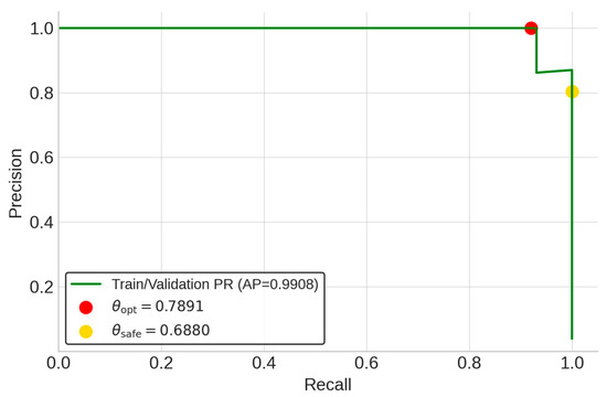
Figure 3.
LR precision–recall curve.
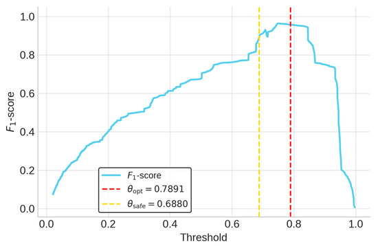
Figure 4.
LR F1-score vs. threshold.
The red marker highlights the optimal balance point at θopt = 0.7891, while the yellow marker indicates θsafe = 0.6880, corresponding to perfect recall (recall = 1.0000). In Figure 4, which plots the F1-score against the threshold, the red dashed line at θopt lies within the F1 curve peak region, confirming that the model achieves high and robust performance from the cross-validation process.
5.3.2. Final Model Performance on Test Set
To verify the model’s generalization capability, it was evaluated on the unseen test set using the two thresholds derived previously. The results, detailed in Table 5, confirm high predictive accuracy.
Table 5.
LR test set performance.
Applying θopt, the classifier achieved 99.94% accuracy. It correctly identified all 1542 non-violation cases and missed only one of the 220 violations, yielding precision of 1.0000 and recall of 0.9955. Using θsafe, the classifier correctly identified all 220 violations (recall = 1.0000; FN = 0) but raised 45 false positives out of 1542 non-violation cases (FP rate = 2.9%), resulting in precision of 0.8302 and overall accuracy of 97.45%. This explicitly quantifies the security–efficiency trade-off under the safety-oriented setting.
5.3.3. Visualization and Practical Implication of Decision Boundaries
Finally, Figure 5 presents an intuitive visualization of the application of the model. It overlays the S-shaped logistic probability curve onto the test set data, illustrating the sharp decrease in predicted violation probability as VMI increases. The vertical dashed lines represent the tangible decision boundaries derived from the model: VMIDB,opt = 0.7893 and VMIDB,safe = 0.8101. These lines offer clear, data-driven criteria for DSOs to implement distinct operational strategies. The performance-oriented boundary (VMIDB,opt = 0.7893) provides a balanced criterion for routine planning, enabling DSOs to manage resources efficiently by focusing on nodes that pose a high statistical risk of violation without being overly restrictive. The conservative boundary (VMIDB,safe = 0.8101), on the other hand, serves as a critical safety net; to prevent the risks of equipment damage or instability, any system with a VMI below this boundary requires immediate review or corrective action.
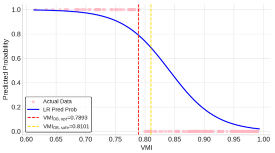
Figure 5.
LR VMI vs. predicted violation probability.
Collectively, these results demonstrate that the proposed framework translates complex system data into a high-performance, interpretable model providing actionable decision boundaries for voltage stability management in distribution systems.
5.4. Benchmarking with Random Forest
To demonstrate that the interpretability of the proposed LR model does not sacrifice predictive power, the LR model’s performance was benchmarked against an RF classifier, a powerful nonlinear model. The RF classifier was trained and evaluated using the same data splits and cross-validation pipeline as the LR model to ensure a fair comparison. The performance of the RF model on the held-out test set is summarized in Table 6.
Table 6.
RF test set performance.
Under θopt, both LR and RF models attain extremely high accuracy, with the LR model slightly outperforming RF (Accuracy = 99.94% vs. 99.72%). In terms of recall, the RF model achieves perfect recall, closely matched by the LR model at 0.9955. Furthermore, the LR model’s VMI decision boundary (VMIDB,opt = 0.7893) differs by only 0.0141 from the RF model’s estimated boundary (VMIDB,opt ≈ 0.8034), underscoring that even when using a powerful nonlinear model, the resulting operating limit remains highly consistent.
Under θsafe, both models achieve perfect recall, ensuring no violation events are missed. Although the RF model attains slightly higher overall accuracy (99.66% vs. 97.45%), this marginal difference is readily acceptable. The LR model’s safety-oriented boundary is VMIDB,safe = 0.8101, while the RF model’s boundary is VMIDB,safe ≈ 0.8063—values that differ only minimally. More importantly, the LR boundary is fully interpretable and derived analytically, enabling transparent risk management and straightforward sensitivity analysis—capabilities not afforded by the RF model’s complex, non-monotonic output.
The fundamental difference in model interpretability is visually captured in Figure 6, which shows the VMI vs. Predicted Probability curve for the RF model. The stepped, non-monotonic shape contrasts sharply with the smooth S-curve of the LR model in Figure 5, making it difficult to extract a simple decision rule from the RF output. Benchmarking confirms that the LR model delivers predictive performance on par with the more complex RF model. It therefore represents a superior approach by combining comparable accuracy with full interpretability and analytically derived, actionable boundaries.
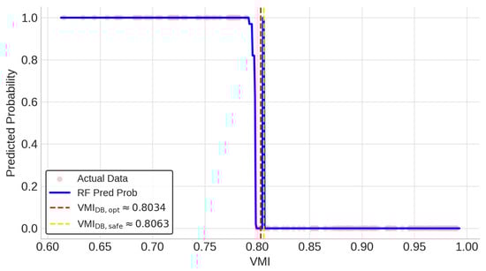
Figure 6.
RF VMI vs. predicted violation probability.
6. Conclusions
This paper proposes a decision-support framework for distribution system operations that uses the VMI as the sole explanatory feature in the LR model. The VMI was chosen because it is a physically meaningful index that synthesizes the combined effects of variables such as load level, DER output, and line conditions—enabling a single variable to effectively capture the system’s voltage state. The LR was selected for its interpretability and analytic invertibility: the model’s closed form enables analytical conversion of calibrated probability thresholds into explicit VMI decision boundaries, a capability unavailable in black-box models. Operationally, LR maps VMI to P(violation). Using the closed-form logit, a calibrated probability threshold is then analytically inverted into an absolute, operator-ready VMI boundary. To balance statistical rigor and operational performance, the workflow comprises two stages: an inferential phase that confirms the VMI’s predictive strength (p < 0.001) and conducts penalized-likelihood-based approximate inference, and a calibration phase that trains a performance-optimized classifier with balanced sample weighting. Extensive time-series simulations of the Jeju Island model generated 8816 samples across six service areas. The 5-fold cross-validation with group splitting produced θopt = 0.7891 and θsafe = 0.6880. These thresholds were then analytically inverted to obtain decision boundaries for the VMI: VMIDB,opt = 0.7893 and VMIDB,safe = 0.8101. On the independent 20% test set, the LR classifier achieved 99.94% accuracy and F1 = 0.9977 under θopt, and 97.45% accuracy with recall = 1.000 under θsafe. To benchmark interpretability against predictive power, the RF classifier was trained on the same data set. Under its θopt, the RF classifier achieved 99.72% accuracy and F1 = 0.9888, and under its θsafe, it achieved 99.66% accuracy with recall = 1.000. The RF classifier’s near-identical performance confirms that the transparent, closed-form LR framework incurs no accuracy penalty compared with a more complex black-box model.
This study establishes a transparent and analytically explicit relationship between the VMI and violation probability via the closed-form LR model. Analytical derivation of the VMI decision boundaries enables practical, immediate deployment across diverse operational scenarios. For routine monitoring, where the cost of a false alarm is low and only a brief verification is required, VMIDB,opt offers a balanced criterion that avoids unnecessary alerts while maintaining high accuracy. For high-stakes decisions such as DER interconnection approvals or infrastructure reinforcement, where a single oversight could have catastrophic consequences, VMIDB,safe enforces zero false negatives and ensures that no real violation is overlooked. Together, these statistically substantiated boundaries replace subjective judgment with clear and reproducible criteria, significantly reducing both ambiguity and subjectivity in voltage management policies.
In our case study, voltages were available for all modeled nodes via OpenDSS, but the framework does not require full observability in practice. Because the LR-derived boundaries are system-level scalar thresholds, operators can apply the same threshold to whatever node voltages are available; where measurements are sparse, proxy locations or lightweight state estimation can provide interim VMI, and under uncertainty the safety-oriented boundary offers a conservative default.
Despite the strong results obtained on the Jeju Island testbed, the generalizability of the framework must be demonstrated across feeders with varied configurations and DER penetration levels. The LR-based VMI decision boundary framework will be applied to urban, rural and mixed network topologies to evaluate and, if necessary, refine the decision boundaries VMIDB,opt and VMIDB,safe for varying grid characteristics and regulatory constraints. In parallel, real-time telemetry from the Advanced Distribution Management System (ADMS) and Phasor Measurement Unit (PMU) will be integrated into a hybrid simulation–live data platform, enabling continuous VMI updates and periodic recalibration of the decision boundaries. These extensions are expected to enhance the robustness, adaptability and real-time applicability of the VMI-based decision support framework, providing DSOs and VPP operators with reliable, data-driven insights.
Author Contributions
Writing—original draft preparation, J.-H.N.; methodology, J.-H.N.; data curation, Y.-J.C.; validation, D.-I.C.; supervision, W.-S.M.; writing—review and editing, W.-S.M. All authors have read and agreed to the published version of the manuscript.
Funding
This work was supported in part by the Korea Institute of Energy Research under Grant C5-2421.
Data Availability Statement
The original contributions presented in this study are included in the article. Further inquiries can be directed to the corresponding author.
Conflicts of Interest
The authors declare no conflicts of interest. The funder had no role in the design of the study; in the collection, analyses, or interpretation of data; in the writing of the manuscript, or in the decision to publish the results.
References
- Sun, H.; Guo, Q.; Qi, J.; Ajjarapu, V.; Bravo, R.; Chow, J.; Li, Z.; Moghe, R.; Nasr-Azadani, E.; Tamrakar, U.; et al. Review of challenges and research opportunities for voltage control in smart grids. IEEE Trans. Power Syst. 2019, 34, 2790–2801. [Google Scholar] [CrossRef]
- Goh, H.H.; Chua, Q.S.; Lee, S.W.; Kok, B.C.; Goh, K.C.; Teo, K.T.K. Evaluation for voltage stability indices in power system using artificial neural network. Procedia Eng. 2015, 118, 1127–1136. [Google Scholar] [CrossRef]
- Junior, W.; Coimbra, A.P.; Wainer, G.A.; Neto, J.C.; Cararo, J.A.G.; Reis, M.R.C.; Santos, P.V.; Calixto, W.P. Analysis and adequacy methodology for voltage violations in distribution power grid. Energies 2021, 14, 4373. [Google Scholar] [CrossRef]
- Pandey, A.R.; Verma, K. Determining locational hosting capacity of DERs in distribution system using machine learning. In Proceedings of the 2024 IEEE Region 10 Symposium (TENSYMP), New Delhi, India, 27–29 September 2024; pp. 1–6. [Google Scholar] [CrossRef]
- Zhang, N.; Jia, H.; Hou, Q.; Zhang, Z.; Xia, T.; Cai, X.; Wang, J. Data-driven security and stability rule in high renewable penetrated power system operation. Proc. IEEE 2023, 111, 788–805. [Google Scholar] [CrossRef]
- Qammar, N.; Arshad, A.; Rehman, A.U. Assessing LV grid PV hosting: A machine learning perspective. In Proceedings of the 2025 International Conference on Emerging Power Technologies (ICEPT), Topi, Pakistan, 10–11 April 2025; pp. 1–6. [Google Scholar] [CrossRef]
- Singh, A.; Singh, P.; Agrawal, N.; Gupta, P. Estimating the stability of smart grids using optimised artificial neural network. In Proceedings of the 2023 International Conference on Recent Advances in Electrical, Electronics & Digital Healthcare Technologies (REEDCON), New Delhi, India, 1–3 May 2023; pp. 380–384. [Google Scholar] [CrossRef]
- Zhu, L.; Lu, C.; Luo, Y. Time series data-driven batch assessment of power system short-term voltage security. IEEE Trans. Ind. Inform. 2020, 16, 7306–7317. [Google Scholar] [CrossRef]
- Geth, F.C.; Akkari, S.; Bletterie, B.; Kadam, S.; Leemput, N.; Papaefthymiou, G. On the Classification of Low Voltage Feeders for Network Planning and Hosting Capacity Studies. Energies 2018, 11, 651. [Google Scholar] [CrossRef]
- Wang, Y.; Zhang, N.; Wang, Z.; Qiu, Z.; Wang, K.; Li, J. Transient Stability Assessment of Power Systems Built upon Attention-Based Spatial–Temporal Graph Convolutional Networks. Energies 2025, 18, 3824. [Google Scholar] [CrossRef]
- Tang, J.; Liu, J.; Wu, J.; Jin, G.; Kang, H.; Zhang, Z.; Huang, N. RAC-GAN-Based Scenario Generation for Newly Built Wind Farm. Energies 2023, 16, 2447. [Google Scholar] [CrossRef]
- Lakshmi, S. Multi-objective optimization approach for EV hosting capacity maximization of distribution networks with renewable generations. In Proceedings of the 2025 IEEE 1st International Conference on Smart and Sustainable Developments in Electrical Engineering (SSDEE), Dhanbad, India, 28 February–2 March 2025; pp. 1–6. [Google Scholar] [CrossRef]
- Zhang, X.; Liu, W.; Wu, L.; Liu, H. Applied Research on Distributed Generation Optimal Allocation Based on Improved Estimation of Distribution Algorithm. Energies 2018, 11, 2363. [Google Scholar] [CrossRef]
- Prasad, M.; Rather, Z.H.; Razzaghi, R.; Doolla, S. A new approach to determine feasible operating region of unbalanced distribution networks with distributed photovoltaics. IEEE Trans. Power Deliv. 2025, 40, 1493–1504. [Google Scholar] [CrossRef]
- Yang, Y.; Huang, Q.; Li, P. Online prediction and correction control of static voltage stability index based on broad learning system. Expert Syst. Appl. 2022, 199, 117184. [Google Scholar] [CrossRef]
- Yang, Y.; Long, J.; Yang, L.; Mo, S.; Wu, X. Correction control model of L-index based on VSC-OPF and BLS method. Sustainability 2024, 16, 3621. [Google Scholar] [CrossRef]
- Bizzarri, F.; Brambilla, A.; Gruosso, G.; Maffezzoni, P. Piece-Wise Linear (PWL) Probabilistic Analysis of Power Grid with High Penetration PV Integration. Energies 2022, 15, 4752. [Google Scholar] [CrossRef]
- Abujubbeh, M.; Dahale, S.; Natarajan, B. Voltage violation prediction in unobservable distribution systems. In Proceedings of the 2022 IEEE Power & Energy Society General Meeting (PESGM), Denver, CO, USA, 17–21 July 2022; pp. 1–5. [Google Scholar] [CrossRef]
- Shahoud, S.; Khalloof, H.; Khalouf, R.; Dupmeier, C.; Cakmak, H.K.; Forderer, K.; Hagenmeyer, V. Fast grid state estimation for power networks: An ensemble machine learning approach. In Proceedings of the 2022 IEEE 10th International Conference on Smart Energy Grid Engineering (SEGE), Oshawa, ON, Canada, 10–12 August 2022; pp. 12–18. [Google Scholar] [CrossRef]
- Yan, J.; Wang, B.; Wu, Z.; Ding, Z. Decentralized voltage prediction in multi-area distribution systems: A privacy-preserving collaborative framework. IEEE Access 2025, 13, 92305–92318. [Google Scholar] [CrossRef]
- Shazdeh, S.; Golpîra, H.; Bevrani, H. An adaptive data-driven method based on fuzzy logic for determining power system voltage status. J. Mod. Power Syst. Clean Energy 2024, 12, 707–718. [Google Scholar] [CrossRef]
- Ye, K.; Zhao, J.; Zhang, H.; Zhang, Y. Data-driven probabilistic voltage risk assessment of miniWECC system with uncertain PVs and wind generations using realistic data. IEEE Trans. Power Syst. 2022, 37, 4121–4124. [Google Scholar] [CrossRef]
- Hu, W.; Yang, F.; Shen, Y.; Yang, Z.; Chen, H.; Lei, Y. Dynamic risk assessment of voltage violation in distribution networks with distributed generation. Entropy 2023, 25, 1662. [Google Scholar] [CrossRef]
- Zaidi, A.; Al Luhayb, A.S.M. Two statistical approaches to justify the use of the logistic function in binary logistic regression. Math. Probl. Eng. 2023, 2023, 5525675. [Google Scholar] [CrossRef]
- Nam, J.-H.; Park, S.-J.; Cho, D.-I.; Cho, Y.-J.; Moon, W.-S. Assessing the suitability of distributed energy resources in distribution systems based on the voltage margin: A case study of Jeju, South Korea. IEEE Access 2025, 13, 36263–36272. [Google Scholar] [CrossRef]
- Hosmer, D.W., Jr.; Lemeshow, S. Applied Logistic Regression, 2nd ed.; Wiley: New York, NY, USA, 2000. [Google Scholar]
- Peng, C.-Y.J.; Lee, K.L.; Ingersoll, G.M. An introduction to logistic regression analysis and reporting. J. Educ. Res. 2002, 96, 3–14. [Google Scholar] [CrossRef]
- Scikit-Learn Developers. What’s New in Scikit-Learn Version 1.6.1; Scikit-Learn User Guide, Version 1.6.1. Available online: https://scikit-learn.org/stable/whats_new/v1.6.html (accessed on 7 March 2025).
- Arlot, S.; Celisse, A. A survey of cross-validation procedures for model selection. Stat. Surv. 2010, 4, 40–79. [Google Scholar] [CrossRef]
- Seabold, S.; Perktold, J. Statsmodels: Econometric and statistical modeling with Python. In Proceedings of the 9th Python in Science Conference, Austin, TX, USA, 28 June–3 July 2010; pp. 92–96. [Google Scholar]
- Pedregosa, F.; Varoquaux, G.; Gramfort, A.; Michel, V.; Thirion, B. Scikit-learn: Machine learning in Python. J. Mach. Learn. Res. 2011, 12, 2825–2830. [Google Scholar]
- King, G.; Zeng, L. Logistic regression in rare events data. Political Anal. 2001, 9, 137–163. [Google Scholar] [CrossRef]
- Heinze, G.; Schemper, M. A solution to the problem of separation in logistic regression. Stat. Med. 2002, 21, 2409–2419. [Google Scholar] [CrossRef]
- Fan, R.-E.; Chang, K.-W.; Hsieh, C.-J.; Wang, X.-R.; Lin, C.-J. LIBLINEAR: A library for large linear classification. J. Mach. Learn. Res. 2008, 9, 1871–1874. [Google Scholar]
- Saito, T.; Rehmsmeier, M. The precision–recall plot is more informative than the ROC plot when evaluating binary classifiers on imbalanced datasets. PLoS ONE 2015, 10, e0118432. [Google Scholar] [CrossRef]
- Powers, D.M.W. Evaluation: From precision, recall and F-measure to ROC, informedness, markedness & correlation. Int. J. Mach. Learn. Technol. 2011, 2, 37–63. [Google Scholar]
- Hastie, T.; Tibshirani, R.; Friedman, J. The Elements of Statistical Learning: Data Mining, Inference, and Prediction, 2nd ed.; Springer: New York, NY, USA, 2009; Chapter 10. [Google Scholar]
- Lim, H.; Kim, H.; Sim, J.; Cho, S. An analysis study on the proposal for increasing hosting capacity in distribution feeders. Trans. Korean Inst. Electr. Eng. 2020, 69, 516–522. [Google Scholar] [CrossRef]
- Dugan, R.C.; Montenegro, D. The Open Distribution System Simulator (OpenDSS) Reference Guide; Electric Power Research Institute: Washington, DC, USA, 2020. [Google Scholar]
- Lee, J.-S.; Nam, Y.-H.; Yoon, S.-J.; Kim, C.-S.; Ryu, K.-S.; Kim, D.-J.; Kim, B. A study on the operation characteristic and grid model for demonstration of mixed virtual power plant. In Proceedings of the Fall Conference, Power Technology Division, Korean Institute of Electrical Engineers, Busan, Republic of Korea, 29–30 November 2023. [Google Scholar]
- KPX. Hourly Generation of PV and WT Generator in Jeju. Available online: https://www.data.go.kr (accessed on 10 October 2023).
- H0-Distribution-Standard-0015, 17th rev.; Technical Standards for Interconnection of Distributed Energy Resources to Distribution Systems. KEPCO: Daejeon, Republic of Korea, 2024.
- Firth, D. Bias reduction of maximum likelihood estimates. Biometrika 1993, 80, 27–38. [Google Scholar] [CrossRef]


Disclaimer/Publisher’s Note: The statements, opinions and data contained in all publications are solely those of the individual author(s) and contributor(s) and not of MDPI and/or the editor(s). MDPI and/or the editor(s) disclaim responsibility for any injury to people or property resulting from any ideas, methods, instructions or products referred to in the content. |
© 2025 by the authors. Licensee MDPI, Basel, Switzerland. This article is an open access article distributed under the terms and conditions of the Creative Commons Attribution (CC BY) license (https://creativecommons.org/licenses/by/4.0/).